Application of Transformer-Based Deep Learning Models for Predicting the Suitability of Water for Agricultural Purposes

Abstract

Water is the most vital component for the sustainability of living beings on Earth. From plants to human beings, every single living being on Earth needs water for its survival. In this research, a novel model has been developed in order to predict the suitability of water for agricultural purposes. This research developed the ALBERT Base v2 model for detecting water quality and suitability and a model named the ALBERT Water Potability Detection (ALBERT-WPD) model, customized from the ALBERT Base v2 transformer model. The model was tested using a dataset from Kaggle, and the performance was evaluated. The research used ten parameters. The performance of both models was measured using metrics, accuracy, precision, recall, and F1-score. In this research, traditional models (CNN and RNN) were developed and compared against the ALBERT model to measure its performance and its efficiency in water potability prediction. The findings revealed that the ALBERT models gained higher accuracies than the traditional models: the Base v2 model gained 91% and the altered ALBERT-WPD rendered 96% accuracy. The classification results (precision, recall, and F1-score) obtained for the ALBERT-WPD model for the potability class were 93%, 98%, and 96% and those for the non-potability class were 98%, 95%, and 96%, respectively. The study found that using transformer models for water potability detection procures higher accuracy with the model optimization method. The study concludes that using transformer models (BERT-based) in water potability detection procures higher accuracy (>95%) with fewer parameters in comparison with traditional models (CNN and RNN) which utilize more parameters. The findings show that the transformer models exhibit rapid data processing and handle large datasets efficiently; the handling of such datasets is complicated when using traditional models, as they have vanishing gradient and encounter temporal data loss challenges. Thus, the significance of the proposed research dwells within the use of “transformers” as an advanced machine learning model to predict water potability and quality, showing that transformers are the future of machine learning.

1. Introduction

Life is based on water, which is the most crucial substance that keeps living beings alive. It is imperative that everyone consumes pure and clean water. Water pollution originates from both natural and human sources, leading to the contamination of numerous bodies of water. People’s health and protection from numerous diseases depend on the removal of these pollutants from water sources. The main causes of water pollution are chemical discharges and heavy metals from factories and industrial units. Water contamination is the primary cause of the water crisis. It must not be contaminated to the point where it cannot be utilized for drinking water or irrigation [1]. Chemical, biological, or physical reactions are the results of water pollutants. Water contaminants have the ability to travel through many water reservoirs as water moves through the water cycle. Since river water only stays in a given reservoirs for a brief amount of time, there is typically only minor contamination.

Pollutants have three main origins: their natural existence on Earth, like pollens, desert dust, meteorites, dust storms, forest fires, wild fires, volcanoes, plant decay, and more [2]; their transformational development into other forms like microorganisms, bacteria, fungi, algae, etc., which are transferred to the air, plants, metals, and food products [3]; their synthesis by humans, e.g., noise, air, and environmental pollutants, arsenic, and more from vehicles, chemical manufacturing and dumping, dry cleaning, and the emission of gases [4]. It is possible that the particles will naturally arise and contribute to the exposure levels of the ecological backdrop. Many of them are detoxified or eliminated by organisms. Examples of naturally occurring contaminants are heavy metals and nitrogen oxides and other radioactive substances and hydrocarbons. Many chemicals are human-made [5], and the pollution they create is not something that occurs in nature. Together with other sources, both direct (intentional harms like toxic waste released into water bodies) and indirect (naturally occurring harms like fertilizers from agricultural land carried off through water ending up in ditches or water bodies), these forms of water pollution are the main causes of contamination [6]. One way that fluids can create direct pollution is when polluted water or toxic substances combined with water are released straight into a river or sea, making the water toxic [7]. Pollutants that wind up in the water incidentally (i.e., as indirect pollutants rather than as direct pollutants) are a major source of water contamination. Chemicals from pesticides and fertilizers are examples of this [8]; these slowly permeate the soil, enter groundwater, and then end up in different watercourses.

The accurate analysis of stream or river water quality is attracting the interest of international pollution control boards and governmental agencies because of its practical uses in assessing the health of watersheds, biodiversity, ecology, and the suitability of the river basin for potable water requirements. Enhancing water quality will require the prevention of uncontrolled trash deposition from industry and routinely monitoring and inspecting streams [9]. Stream meandering, multidimensional mixing, evaporation, and turbulence are only a few of the several additional elements that impact stream water quality [10]. Major river basins, such as the Ganga, Yamuna, and Cauvery in India, have been examined for their water quality parameters (WQPs) [1,11]. The tests showed that the water quality of the Ganga and Yamuna rivers is “poor”, with high concentrations of Na and Cl ions and severe pollution from sewage discharge and wastewater, whereas the Cauvery River alone meets water quality standards. There have been reports that the main factor contributing to the decline in water quality is a high biochemical oxygen demand (BOD) level from the dirty sewage that metropolitan areas dispose of. In this regard, authors [12] used an artificial neural network (ANN) for predictions of stream water quality, and the proposed method is proven to be effective in predicting water quality using 22 parameters: pH, dissolved oxygen (DO), conductivity, biochemical oxygen demand (BOD), chemical oxygen demand (COD), nitrate, coliform, turbidity, alkalinity, chloride, hardness, calcium, magnesium, sulfate, sodium, total dissolved solids (TDSs), total suspended solids (TSSs), phosphate, potassium, fluoride, sodium %, and sodium adsorption ratio (SAR).

Heavy metal concentrations in sewage wastewater, industrial wastewater discharges, and air deposition are quite high due to the quick changes brought on by urbanization [13]. Because of extensive human activity, heavy metal concentrations in soil, water, and sediments are getting worse [14]. Consequently, having an automated framework that can immediately detect water quality is quite vital.

Unsupervised learning makes use of unlabeled training datasets to solve a variety of pattern identification issues. In order to distinguish between clean and contaminated water based on water images, the authors proposed an attentional neural network (supervised) which focused on a convolutional neural network (CNN) [15]. The model used water-pollution-based images as inputs and classified the polluted images and non-polluted images. The study did not use physical- or chemical-based properties as parameters and achieved accuracies of 66.4% and 63.2% for the proposed models, respectively. Artificial neural networks and support vector machines (SVMs) [16] have been proven to be effective in the analysis of water quality components. One study reviewed the results and concluded that among the supervised and unsupervised water quality prediction models, the XGBoost models based on decision trees (DTs) procured higher accuracy than models based on artificial neural networks (ANNs), support vector machines (SVMs), k-nearest neighbors (KNNs), and random forest (RF) approaches.

Understanding market interest in water quality and accessibility from a variety of sources is necessary to balance the water market. Rapid development has led to an unsettling pace of decline in water quality. One of the key theories for the rise in terrifying illnesses has been identified as helpless water quality results. Using supervised machine learning, a model is proposed for predicting water quality [17]. Their research used four parameters: turbidity, pH, temperature, and total dissolved solids (TDSs). Utilizing 15 different ML algorithms (linear regression, polynomial regression, random forest, SVM, RF, ridge regression, elastic-net regression, multi-layer perceptron (MLP), gradient boosting (GB), Gaussian Naive Bayes, stochastic gradient descent (SGD), logistic regression, decision tree, bagging classifier, and k-nearest neighbor), the authors developed a different model. Among the fifteen developed ML models, the GB model, with a learning rate (lr) of 0.1, achieved a mean absolute error (MAE) of 2.7273; the polynomial regression model, with a degree-of-freedom (df) of 2, achieved an MAE of 1.9642. In contrast, the MLP model achieved the highest accuracy (85%) among the fifteen models. The polynomial regression and GB models predicted the best WQI (Water Quality Index), whereas the MLP predicted the best Water Quality Class (WQC). Thus, they concluded that ML models with minimal parameters achieve reasonable accuracy in real-time scenarios. The authors presented a machine-learning-based classification model for water quality [18]. Based on AI computations, the article suggests a plausible grouping model for ranking the quality of water. The author developed five models (Bayes, Rules, Trees, Lazy, and Meta) with data from the KDD (Knowledge Discovery in Databases) databank and their performances were compared. Among the models, the K-Star algorithm based the Lazy model gained a higher accuracy of 86.67% in water quality classification. The data included 54 parameters. The attributes included the following: DO, turbidity, sodium, color, lead, pH, time, latitude, and longitude. The authors proposed a model using pH, turbidity, temperature, and TDS boundary sensors to transmit data via an Arduino microcontroller and a ZigBee communication device [19]. They used five different methods based on the following approaches: Naive Bayes, gradient boosting, deep learning algorithms, random forest, and decision trees. Once the models predicted water quality, the results were examined, and users were notified through an IoT-based ZigBee handset developed by the authors for water monitoring. Thus, in addition to detecting low-quality water, the paper also focused on alerting the users of the system (water-quality-concerned professionals) when the water was ready for use.

The current research thus contributes the knowledge of utilizing larger datasets with a natural-language-processing-based transformer model to predict water potability. CNN, RNN, and ANN architectures (as traditional methods) were the only methods being used to predict water quality and potability until recently. By adopting BERT and BERT-based advanced ML models, the challenges that are encountered in using traditional models like CNN and RNN (namely vanishing gradient, huge data loss (temporal loss of data) occurrences, and time-consuming processing for handling larger and complex datasets) are rectified. Also, future advancements and creations, with increasing challenges and complexities, require ML models that can predict abnormalities, surpassing the outcomes of traditional models. Hence, adopting a novel, advanced ML model architecture (transformer) is a suitable approach for the here-proposed research objectives. This research attempts to develop and use ALBERT-based transformer models to predict water quality and potability, presenting a novel approach. The research aims to develop a model with higher accuracy (>95%) and minimal loss, using an ALBERT-based transformer prediction model; this can be used as a reference point for future research utilizing transformer models, and the results presented here can be used in comparative analyses.

The first section covers the research background, significance, novelty, purpose, and aim of the research. The second section presents a literature review, where existing water quality prediction models, relevant research, and usage of different algorithms to predict water quality are examined and reviewed. In the third section, addressing methodology, details are provided on the evaluation metrics used, the datasets and statistical methods adopted, the architecture developed, and the algorithms proposed; furthermore, detailed descriptions of the model will be provided. The fourth section includes the results (loss and accuracy estimation) and data analysis (performance analysis). The fifth section will be focused on data analysis of different models using the same datasets. Finally, the last section describes the conclusion, limitations, and implications.

2. Literature Review

Machine learning has been shown to be a useful tool for activities like data analysis, classification, and predictive analysis due to the fast increase in availability of data pertaining to aquatic habitats. Machine-learning-driven models, as opposed to traditional models, employed in water-focused research excel at solving complex nonlinear issues quickly. The design, monitoring, modelling, assessment, and improvement of various water treatment and management systems are just a few of the activities where insights and models created by machine learning have found use in the field of water environment research. Additionally, machine learning offers practical solutions for problems relating to reducing water pollution, improving water quality, and safely managing watershed ecosystems; examples of these solutions include plastic waste reduction, reducing herbicides and pesticides, wastewater treatments, water conservation, water purifications processes, and implementation of water-efficient toilets [16].

2.1. Major Pollutants in Water Bodies

Water that is unsafe and unfit for drinking or for important applications like agriculture is referred to as polluted water. Over 500,000 people die worldwide every year from diseases including polio, cholera, dysentery, typhoid, and diarrhea as a result of polluted water. The main sources of water contamination include bacteria, viruses, parasites, pesticides, fertilizers, medicines, phosphates, nitrates, plastics, feces, radioactive elements, and even fertilizers and pesticides. These substances frequently qualify as hidden contaminants since they may not obviously change the color of the water [20].

2.2. Machine Learning Approaches to Identify Pollutants in Water Bodies

A Northern California watershed was contaminated with microorganisms, which were evaluated using various machine learning models in a study by [21]. The study examined the associations among the variables (i.e., hydrological variables, land cover, weather, and microbial sources) as inputs. The authors developed models based on XGBoost, K-nearest neighbors, Naive Bayes, support vector machine, simple neural network, and random forest. Parameters like human or nonhuman microbial sources were effectively classified by the models, with accuracies ranging from 69% to 88% (Naive Bayes). In receiver operating characteristics (ROCs) analysis, XGBoost outperformed random forest and k-nearest neighbor (KNN), with an average area under the curve (AUC) of 0.88.

The main goal of the study conducted by the authors [22] was to use geographic information, such as the location and elevation of water bodies, as input variables in various machine learning approaches for forecasting pollution. The study assesses and examines the findings in relation to groundwater pollution and site-specific chemical makeup. To anticipate variables like pH, temperature, turbidity, dissolved oxygen, hardness, chlorides, alkalinity, and chemical oxygen demand, immutable elements like latitude, longitude, and elevation can be used. There have not been many studies that have taken location-based criteria into consideration for predicting water pollution. The main objective in their research is to establish a link between geographic characteristics and their impacts on water pollution in a specific area. Among the different models, the result of the SVM model gained an R2 training score of 99.65 and a testing score of 29.87, which are higher than those attained using other models (multivariable, lasso-regressor, and DT). The study concluded that SVM with particle swarm optimization enhances predictions of water quality.

Other different ML techniques used in predicting water pollutants via quality and potability prediction were reviewed here (refer to

Table 1. ML techniques used to identify water pollutants.

Author and Year	Machine Learning Technique/Model Architecture	Parameters	Prediction Class	Accuracy/Results
Ma et al. [23]	Hybrid: deep neural networks (DNNs) + deep matrix factorization (DMF)	Biological Oxygen Demand (BOD), turbidity, Ecoli, coliform, fluoride, chlorine, and dissolved oxygen (DO).	Biological Oxygen Demand (BOD)	RMSE scores: 17.23% and 25.16% lower than the traditional and conventional ML models, respectively.
Ly et al. [24]	Adaptive neuro-fuzzy inference system (ANFIS), regression models (SVR, DTR, and linear), deep learning (GRU, RNN, and LSTM), and time–series (SARIMAX)	Twenty parameters: COD (chemical oxygen demand), BOD (bio-chemical oxygen demand), TSS (total SS), TOC (total organic carbon), TP (total phosphorus), TN (total nitrogen), pH, DTP (dissolved TP), DTN (dissolved TN), PO4 (phosphates), NO3 (nitrates), NH3 (ammonia), Fcoli, Tcoli, temperature, DO (dissolved oxygen), electrical conductivity (EC), precipitation, chlorophyll-a (Chl-a), and flow rate.	Eutrophication and algal blooms	ANFIS obtained the highest accuracy, 90% (MAE = 0.090).
Park et al. [25]	SVM, artificial neural networks (ANNs)	Chl-a, NO3-N, PO4-P, NH3-N, wind speed, temperature, and solar radiation.	Chlorophyll-a (Chl-a) Concentration	SVM obtained a more accurate prediction than ANN.
Krivoguz [26]	Six different machine learning algorithms (kNN, RF, SVM, NN, decision tree, and logistic regression)	Salinity of sea surface, Chl-a, temperature, DO, PO4, NH3, and NPP (net primary product).	Dissolved oxygen (DO)	Random forest with AUC: 0.996.
Göz et al. [27]	Extreme Learning Machine (ELM) and Kernel Extreme Learning Machine (KELM)	pH, temperature, conductivity, and DO.	Dissolved oxygen (DO)	KELM procured higher success in predicting DO, with an R-test score of 0.9855, an MAPE-test score of 2.8471, and an RMSE-test score of 0.3807.
Moon et al. [28]	AdaBoost, random forest, and gradient boosting.	Nine parameters: pH, SS, DTP, TN, NH3-N, temperature, COD, DTN, and NO3-N.	Optimal water quality (WQ)	CVRMSE: 17.404; R2: 0.912.

Note(s): Source: Author.

).

Table 1 provides a small glimpse of the different water quality prediction and potability results along with details used in monitoring and assessing the machine learning models. These models were developed using traditional approaches like support vectors (machines, regressor and classifiers), regression methods (linear and logistic), nearest neighbors, decision trees, and simple neural networks.

The authors [23] developed a hybrid model using a deep neural network (DNN) + deep matrix factorization (DMF) approach, with seven variables: Biological Oxygen Demand (BOD), turbidity, Ecoli, coliform, fluoride, chlorine, and dissolved oxygen (DO). The research used sparse matrix approach for data analysis, since there were missing values for BOD. After pre-processing the 148,892 samples accumulated from NYC database, the valid (i.e., non-missing values) 32,323 data samples, both before and after update, were obtained from 2018; then, 285 samples were added and used in their research (totaling 32,608 samples). The BOD over five days was used for prediction and detection since it is a statistically complicated and tedious process. The performances of the models were evaluated using RMSE estimation. The proposed DNN + DMF model gained a lower RMSE score (17.23%) than the traditional ANN and SVM ML models and, similarly, a lower RMSE score (25.16%) than the conventional kNNand ensemble ML models, respectively.

The authors [24] developed an adaptive neuro-fuzzy inference system (ANFIS) as their main model and compared their results with those of other developed models like regression models (SVR, DTR, and linear), deep learning (GRU, RNN, and LSTM), and time–series (SARIMAX) models. The research used twenty parameters: COD, BOD, TSS, TOC, TP, TN, pH, DTP, DTN, PO4, NO3, NH3, Fcoli, Tcoli, temperature, DO, EC, precipitation, Chl-a, and flow rate. The data collection and processing took ten years; the samples were collected from Han River, South Korea. The classification analysis was performed based on ‘Eutrophication and Algal Blooms‘. The datasets were pre-processed and analyzed using mean accuracy error (MAE) estimation. Among the models, ANFIS obtained the highest accuracy of 90% (MAE = 0.090).

The study by authors [25] focused on Chl-a concentration prediction in water quality. The samples were collected from estuarine (Yeongsan Reservoir) and freshwater (Juam Reservoir) reservoirs of Korea. The timeline of the meteorological data collection was charted as 7 years. They developed two models, SVM and ANN. The parameters used here are Chl-a, NO3-N, PO4-P, NH3-N, wind speed, temperature, and solar radiation. The chlorophyll-a (Chl-a) concentration was the target value (output) for the prediction models. Of the two models, the SVM gave more accurate predictions than ANN. The models they developed were based on prediction and early-warning protocol of water quality that examined Chl-a concentration.

The authors [26] developed six ML-algorithm-based models using kNN, RF, SVM, NN, decision tree, and logistic regression methods. The parameters used here were the following: salinity of sea surface, Chl-a, temperature, DO, PO4, NH3, and NPP (net primary product), where the DO is the output parameter. The data obtained were from the 1992–2019 timeline and were gathered from the CMEMS databank using Black Sea areas as sources. The data were analyzed using AUC and ROC methods for evaluating the models’ performances. Among the six models, the RF gained a higher accuracy rate with AUC: 0.996 (99.6%) followed by kNN (98.8%), Tree (95.9%), NN (95.6%), LR (71.3%), and SVM (48.6%). Thus, they concluded by stating that the RF model predicted DO accurately; among the factors used, temperature, salinity, and phosphates were crucial in identifying the DO concentration fluctuation in Black Sea areas.

Study by [27] focused on predicting DO using two artificial intelligence (AI) models, Extreme Learning Machine (ELM) and Kernel Extreme Learning Machine (KELM). The parameters used here are pH, temperature, conductivity (EC), and DO. Dissolved oxygen (DO) was the output parameter. The study employed sigmoid, sinusoidal, radial basis, hard-limited, and triangular basis functions for data analysis in the ELM model. Similarly, in the KELM context, the researchers adopted radial basis and linear kernel functions. Among the two models, KELM procured higher success in predicting DO, with an R-test score of 0.9855, an MAPE-test score of 2.8471, and an RMSE-test score of 0.3807; the ELM model gained an R-test value of 0.9481, an MAPE-test value of 7.1997, and an RMSE-test value of 0.7261.

The authors [28] initiated the development of an algorithm for predicting optimal water quality in Hwanggujicheon Stream. The study employed the AdaBoost algorithm for water quality prediction using various input variables. The inputs used were water temperature, pH, SS, TN, NH3-N, DTN, DTP, COD, and NO3-N. The study was carried out with the aim of exploring the DO prediction (target: output) in an urban river (Hwanggujicheon Stream) using the ML model. AdaBoost, known for its strong predictive performance, was selected over other models. The results obtained were R2 = 0.912, RMS = 0.015, coefficient variation RMSE (CVRMSE) = 17.404, and MAE = 0.009. As per the performance evaluation methods adopted, the R2 value was closer to ‘1’ and CVRMSE was <30 according to the ASHARE guidline-14 criteria. This showed that utilizing the AdaBoost model procures reasonable accuracy in water quality prediction with minimal loss.

2.3. Research Gap

One area of research that has been neglected in the literature on machine learning applications for pollution and water quality prediction is the poor integration of different data sources. Several studies like [15,23,26,27], have focused on physical and chemical (physicochemical) attributes: solids, temperature, odor and taste, color, turbidity, salinity, heavy metals, DO, BOD, COD, ions, hardness, pH, alkalinity, electrical conductivity, etc. Similarly, studies [6,29,30,31,32,33] have examined geographical information along with physicochemical factors, with a focus on parameters like latitude, longitude, DO, turbidity, suspended particles, and phytoplankton.

In order to address water quality and pollution problems, machine learning models and cutting-edge strategies need to be used. A few of the predictive models that have shown success in evaluating and forecasting water quality metrics (including microbial contamination, dissolved oxygen levels, and pollutant sources) are AdaBoost [34], XGBoost [35], and Extreme Learning Machine [36]. Existing water-quality-based research has focused on either CNN-, RNN-, or ANN-based traditional ML models, and the lack of advanced ML models and especially transformer-based NLP models in detecting water potability and quality have paved the way for the proposed research. Research into cutting-edge machine learning techniques will be crucial in addressing water quality and pollution issues in the future.

The scalability, adaptability, and potential of machine learning models for early warning systems and real-time monitoring for the management of water quality need to be investigated via extensive research. The adoption of different ML models than CNN, building hybrid models with different deep learning algorithms, and the use of different neural networks are identified as the major areas that are lacking in the existing literature. Such research could be particularly crucial in heavily populated regions, where pollution and water quality issues are becoming worse. The proposed study exclusively focuses on water potability (for human consumption of water: drinking water); thus, by focusing on the necessary factors (water potability attributes) as parameters by using a different ML approach (ALBERT: A Lite BERT) than the existing ones is an attempt to bridge the literary gap. The nonexistence of BERT (transformer-based architecture) models in water potability prediction thus adheres to the research gap.

3. Materials and Methods

The methodology section includes information about the datasets used, the algorithms adopted, the architecture developed, and the model built. In this research, two models have been developed: one is ALBERT Base v2 and the other is a model with layer modifications of ALBERT Base v2 which has been named the ALBERT V2 Water Potability Detection (ALBERT-WPD) model.

3.1. Dataset and Parameters Used

The datasets for the current research have been obtained from the resource ‘kaggle’, where author [37] has provided data for water assessments and measurements related processes. The datasets are used for research focusing on analyzing and measuring the pollution level, human consumption suitability, and potability (potable-water is water that is safe and clean to drink) in general. The author collected datasets of water potability from the data repository [38] that has 3276 datasets. The dataset is split into an 80:20 ratio. The ten parameters (presented in the Parameters column of

Table 2. Datasets adopted.

S. No	Parameters	Float Type and Parameter Type	Description	Compound/Property
1	pH	Input; float64	Water‘s potential of hydrogen level	Chemical compound
2	Chloramines	Input; float64	Concentration of chloramines in water	Chemical compound
3	Solids	Input; float64	Solids completely dissolved in water	Physicochemical property
4	Hardness	Input; float64	Mineral-content-measurement-based water hardness	Physicochemical property
5	Conductivity	Input; float64	Water’s electrical conductivity	Physical property
6	Sulphate	Input; float64	Concentration of Sulphates in water	Chemical compound
7	Trihalomethanes (THMs)	Input; float64	Concentration of the tri-halo-methane in water	Chemical compound
8	Organic_carbon	Input; float64	The organic-carbon-based contents present in water	Physicochemical property
9	Turbidity	Input; float64	Measurement of water clarity or the turbidity level	Physical property
10	Potability	Output: int64‘	‘Target level’ in research with ‘0’ being not potable and ‘1’ being potable	Physicochemical property

Note(s): Source: Author.

) used here are presented in Table 2.

The data obtained from kaggle are verified and analyzed here for reliability and validity using correlation and univariate analysis; they are represented using histogram charts in the data analysis section. The datasets obtained are cross-verified for missing values. Using missing value function as “dataframe.isnull().any()”, the research fills in the missing values in cells of data frames in python. Once the values are complete, they are loaded in the model for prediction.

Since the current research focuses on water-quality- and potability-based pollutant assessment, all ten parameters are used here. Using the values obtained from the repository, the water pollutant or the potability level is estimated as ‘target’ value where potable (1) and not potable (0) classification is carried out. The datasets are pre-processed and available for use in the ALBERT Base v2 and ALBERT Water Potability Detection (ALBERT-WPD) models for classification.

The target value potability is estimated based on the WHOs (World Health Organizations) standard [39,40,41] (refer

Table 3. Parameters with units and WHO standards.

S. No	Parameters	WHO Standards (with Units)
1	pH (calculated using a scale ranging from 0 to 14 to measure the alkalinity or acidity of substances; where 0–6 = most acidic; 7 = neutral and >7 = basic)	6.5–8.5
2	Solids	500–1000 milligram/liter (mg/L)
3	Chloramines	4 mg/L
4	Sulfate	3–30 mg/L in freshwater & 2700 mg/L in seawater
5	Conductivity	400 µS/cm (Microsiemens/centimeter)
6	Organic_carbon	<2 mg/L to <4 mg/L
7	Trihalomethanes	80 ppm (parts per million)
8	Turbidity	0.98–5.00 NTU (Nephelometric Turbidity unit)
9	Hardness (water with calcium carbonate concentrations: CaCO3 is measured here)	120–170 mg/L

Note(s): Source: Author.

).

Based on the results, the water potability is classified as ‘0’ and ‘1’ by the model and thus, later, the water quality is classified into potable (1) and not potable (0) classes, respectively.

3.2. Training

Data training here includes fine-tuning parameters for optimal performance and training the model to obtain less data loss without overfitting issues. To achieve these two phases, the current research adopts larger epochs for the training rate and the learning rate (LR).

The current research chose 100 epochs since the model uses large datasets. Also, since the transformer model is the first attempt in water potability prediction, when monitoring the model performance, attempts to prevent or address the overfitting issues (callback function) are considered here. The authors [42] stated in their study that adopting 50–100 epochs for large data is a good starting point for training a model. Using an early-stop protocol to monitor the training process and to validate the data and model saves time with 100 epochs. Thus, the study adopts 100 epochs.

Similarly, the learning rate (LR) is set as 0.01 because, according to [43], based on the model architecture and datasets, defining tasks is crucial. Thus, setting the LR as 0.001–0.01 is deemed to be a good starting point in the training phase. The smaller the LR, the slower the learning process, and vice versa. Hence, the optimal range of 0.01 is chosen here for the LR.

3.3. Machine Learning (ML) Models

The ML models in predicting water potability, quality, and level in the past few years have increased due to its significance in handling complex and large datasets [44,45,46,47,48,49,50,51,52,53,54]. The traditional models in assessing and predicting water quality use support vector machine (SVM) models with individual parameters. Hybrid models like the long short-term memory (LSTM) approach with artificial neural network (ANN) and recurrent NN (RNN) architectures were adopted later for more complicated large datasets. The usage of transformers in predicting the water quality and potability has been seldom attempted. Thus, by using ‘A light BERT’ (ALBERT) as a machine learning architecture, the researcher developed two models with integrated parameters for data assessment and evaluated both models to gain a better and more accurate model.

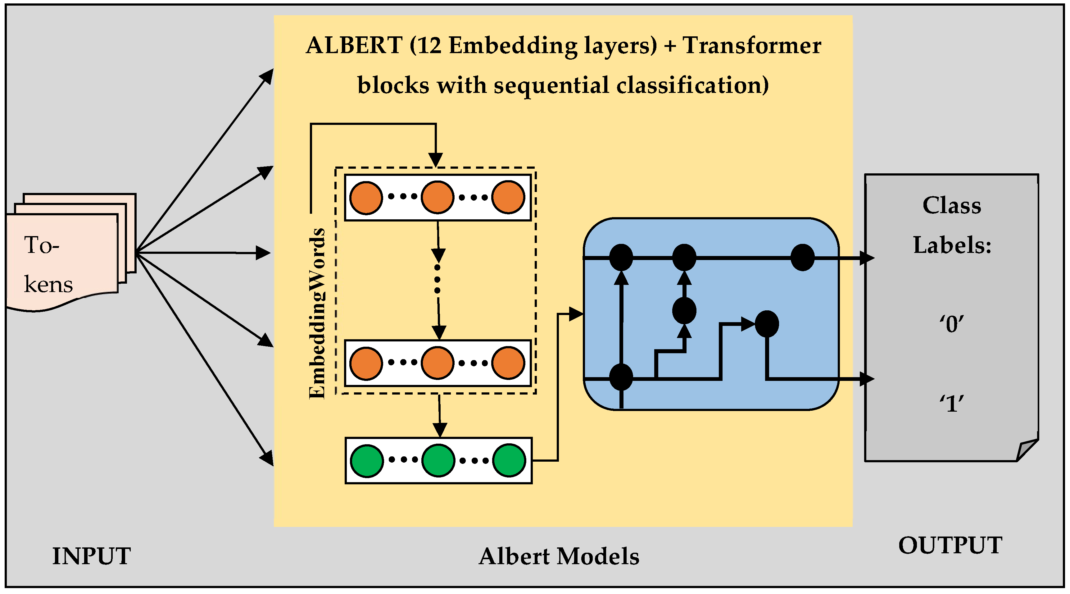
3.3.1. Proposed Architecture

The models proposed in this research are ALBERT Base v2 which is masked language modeling (MLM)-based and a hybrid model using ALBERT Base v2 with sequential layers named ALBERT-WPD. ALBERT model is a natural language processing (NLP)-based transformer where the model is pre-trained with the sentence-ordering prediction (SOP) method [55]. Since the current research is on the prediction of water potability, the numbers (integers) are directly used as tokens prior to processing (i.e., filtering invalid or missing data). ALBERT Base v2 is faster and more, efficient with 128 embedding layers, 11 million parameters, 12 attention heads and repeating layers, and 768 hidden dimensions [56]. Figure 1 represents the scheme of the transformer layers utilized here.

ALBERT Base v2 is a pre-trained English-language-based masked model (MLM). [55] designed and developed the ALBERT Base v2 model in 2019 using BERT as their base reference. It has fewer parameters than BERT_Large and thus works rapidly and reduces computational time. The ALBERT Base v2 model is uncased; meaning that both the lower and upper cases have equivalent values and can be used. ALBERT is a self-supervised learning-based language where mixed inputs and parameters, such as numeric- and text-based predictions, are used. The ALBERT Base v2 is an upgrade of ALBERT Base, where the dropout rates, training data, and training time were improved to meet the initial versions’ drawbacks. This model can be implemented in two major ways: for textual analysis and for fundamental entity analysis. Normally, ALBERT uses text sequences (i.e., sentences) as inputs and converts them into numbers (i.e., integers) for rapid data processing. The final output retrieved is in numeric form [57]. However, here, in the proposed research, the model uses numeric data as tokens, under the fundamental NLP tasks where the inputs are recognized as entities.

In this research, two ALBERT transformer models are built. One is the ALBERT model of Base version2 and the other is the optimized model derived from ALBERT Base v2, where sequential layers and optimization are included. The developed model is the custom model with modifications in layers of ALBERT Base v2, named the ALBERT V2 Water Potability Detection (ALBERT-WPD) model. The ALBERT Base v2 model has tokens as input as first layer followed by an embedding layer with 128 feature extraction points. Next, 12 repeating blocks of transformers process the data and send the processed data. The processed data are then passed through linear layers of 768 feature extractions as input and 64 as output in ReLU and 64 feature extractions as input and 1 as output in the sigmoid activation function layer, respectively, to classify the outcomes. The classified result is obtained as an outcome. The proposed custom model’s architecture includes similar layers as those in the ALBERT Base v2 model but with 3 additional layers of ReLU functions (refer to Figure 2).

The difference between BERT and ALBERT is that BERT has 12 unique parameters as transformer blocks, whereas the ALBERT model has 12 repeating blocks. The custom ALBERT model developed (i.e., ALBERT-WPD) includes an input layer where the numeric/integer values are passed through as inputs. Next, the pre-processed inputs are passed through the ALBERT Base v2 model to obtain and further process the values as sentences and pass the same through 4 linear layers with 768 feature extraction as input and 512 as output, 512 feature extraction as input and 128 as output, 128 feature extraction as input and 256 as output, and finally 256 feature extraction as input and 32 as output in the ReLU activation layers. Finally, the outputs are classified using the sigmoid layer with 32 feature extraction as input and 1 as output for classifying the processed data.

The use of the ALBERT model in examining the water quality parameters reduces the data computation constrains. Since the datasets are larger in size, the ALBERT model is used here for data throughput, lower memory consumption, and rapid computations. One significant benefit in adopting ALBERT models in water quality is that they use few parameters, unlike BERT transformer models. Here, the inputs, used as tokens, are processed as ‘entity recognition’ and passed onto the next hidden layers of the models. Here, the parameters used are of the following types: physical, chemical, and physicochemical properties that are classified under “named entity recognition” (NER) tasks. The NLP task in the ALBERT model is the fundamental process, where the input tokens are processed, located, extracted, and then classified as per the predetermined classes, as outputs. The models here examine the threshold values of the parameters, predefined based on the WHO standard values. For example, the pH value, as per the standard, must be within 1–14; based on the WHO criteria, if the values are >8.5, then the water is categorized as being high in ‘alkalinity’; if the value obtained is <6.5, then the water is categorized as being ‘acidic’. Thus, based on NER, the model examines, analyzes, and predicts the water quality and potability to procure final outcomes. When the obtained values (actual) are within the WHO standards (expected), the water is then classified as potable; if not, then it is classified as not-potable. This process is repeated for all the inputs; then, the classification of the model along with its performance are finally evaluated using metrics.

3.3.2. Adopted Traditional Model Architecture

The current study adopts the architectures of traditional models, convolutional neural networks (CNN) and recurrent neural networks (RNNs), for comparing the accuracy obtained with the proposed model, with the aim of proving its efficiency. The CNN model adopted here has a one-dimension (1D)-based single channel for the input layer. The first layer (convolutional layer) has a size of 128 with a kernel size of 3, and a size of 64 with a kernel size of 3. The activation function is set as “ReLU” for each layer. Next is a flatten layer and a dense layer. Lastly, the CNN model has an output layer with a dense layer, a sigmoid activation layer, and a classification layer (refer to Figure 3).

The CNN model is trained using loss (binary-cross_entropy) and accuracy metric to evaluate the performance. Similarly, the model is optimized using an SGD (stochastic gradient descent) optimizer algorithm. There are 100 epochs used for training here, with a batch size of 1. The model uses “callbacks”, which is an early-stopping function that calls back the training of the model when the metrics are not improving. This function trains the model efficiently by not leading to an overfitting issue in the data. Thus, we were able to achieve a reduction in the use of computational resources while attaining a higher performance.

The next traditional neural networking model adopted here is the RNN. The RNN model here has input, LSTM (long short-term memory), and output layers using sequential networking layers. The first layer (input) in this model has a kernel of size of 9 × 1. Next are the LSTM layers, with sizes of 64 and 32, respectively. A batch normalization layer is added to the LSTM layer. The next layer is the ‘dense’ layer, with sigmoid as the activation function (refer to Figure 4). Thus, the model is compiled. Using SGD as an optimizer, binary_cross-entropy as a loss function, and accuracy as a performance metric, the model is compiled and trained. Early stopping as a callback function is used here too. The epochs are set to 100 runs, with a batch size of 1.

The RNN in such a way that the data flow sequentially. The time steps depend on the previous time steps. The RNN working principle passes data sequentially through the hidden LSTM layers in each time step. The RNN has a self-looping (recurrent) workflow, where inputs for predictions in LSTM are remembered by the LSTM layers. Thus, one or more RNNs work to predict water potability and categorize it into two classes: potable and non-potable.

3.4. Machine Learning Algorithms

The major techniques and algorithms used in predicting water quality and potability in the existing ML models are those of SVM [16], NN [12], random forest (RF) [58], decision trees (DTs) [17], multi-layer perceptron (MLP) regressor [17], k-nearest neighbor (kNN) [17], regression techniques [17], Adaptive Boost (AdaBoost) [21], gradient boost (GB) [21], and Extreme Learning Machine (ELM) [27,36]. In this research, a feed-forward algorithm is adopted to operate the sequence model in the developed custom ALBERT-WPD in order to eliminate and select variables to assess potability with minimal loss.

Experimental Procedure

In this section, the different algorithms adopted for training the model, the neural network algorithm, and the classification algorithms will be explained. ‘Python’ was adopted to develop the ALBERT models for water quality prediction. It is an open-source programming language which has several libraries. Initially, once the datasets are acquired, they are pre-processed (invalid data and missing values are filtered out) and loaded via python codes by importing libraries from the Python 3.13.0 Open Source (OS). The following algorithms are used in this research for training the ALBERT models:

Algorithm 1. Feed-forward algorithm

Data split: train and test with parameters = feature ‘x (train), y (test)’, size = 0.05 and random state = 42. Dataset initiation: Train X data with Tokenizer as Input of maximum length 512, and Test Y data with Tokenizer as Input of maximum length 512. Dataset loading: Train data_load with batch size as 64 and set parameter ‘shuffle’ as true; Test data_load with batch size as 64 and set parameter ‘shuffle’ as false.

Algorithm 2. NN algorithm

Step 1: Import python libraries torch and pandas; from torch import NN and Adam optimizer, from sk-learn, import train-test-split, MSE, MAE, R2 metrics, and from transformers import Auto-tokenizer and AutoModel; Step 2: Initiate pre-processing of datasets and pass the pre-processed data as ‘inputvalue’. Initiate the ALBERT Base v2 model; Step 3: Apply sigmoid and ReLU activation functions on data to classify the processed data as output; Step 4: Finally, return the value ‘0’ or ‘1’ as per the obtained output and classify the potability.

The classification algorithm is written as a workflow for better understanding, as presented in Figure 5.

3.5. Metric Evaluation Techniques Adopted

In this section, the evaluation techniques adopted here will be discussed. The research adopts classification accuracy and categorical cross-entropy (log–loss) approaches for evaluating the accuracy and loss in machine learning, respectively. The accuracy is estimated using the classification accuracy proposed by [59]. See Equation (1), where accuracy (acc) is estimated using true positives (tps), true negatives (tns), false positives (fps), and false negatives (fns):

$$ACC={\displaystyle \frac{tps+tns}{tps+fps+tns+fns}}$$

(1)

The losses of the models are estimated using the log–loss method adopted from [60], where the actual and predicted outputs are analyzed and categorized. To minimize the loss value and to classify the results based on the outcomes with higher accuracy, the loss is estimated in research using different approaches; here, the cross-entropy method is suitable and adopted for the classification of the potability of water. In Equation (2), Cl denotes the total number of classes; $t_x$ and ${\widehat{t}}_x$ are the actual and predicted outputs, respectively.

$$Loss=-{\displaystyle {\sum }_{x=1}^{Cl}}{t}_x\log {\widehat{t}}_x$$

(2)

3.6. Importance of Confusion-Matrix

In prediction models, a confusion matrix provides a meticulous breakdown of the data which are analyzed by providing positives and negatives (true and false) as a contingency plan. It allows a researcher to understand the model’s performance in par with real-world consequences, risks, and misclassifications (original versus expected) [61].

A confusion matrix is necessary beyond accuracy estimation, since imbalanced datasets and data errors can lead to misclassifications. Thus, by adopting a confusion matrix, a more nuanced evaluation of model performance can be achieved. Through understanding the misclassifications and errors, the false positives along with false negatives (actual negative outcome) are identified clearly in the confusion matrix, which eradicates real-world consequences, namely misdiagnoses in medical/healthcare predictions (preventing timely care and medications, leading to fatal outcomes) and wrong flagging (legitimate transactions flagged as illegitimate: false positives) in the banking industry, among others. Thus, using a confusion matrix is a significant and important measure in estimating the accuracy of models.

4. Results and Findings

In this section, the accuracy and loss evaluation results of the ALBERT-V2 model and ALBERT-WPD model are compared; similarly, the findings of the obtained evaluation metrics results are represented using a confusion matrix graph and histogram chart.

Hyper-parameters: The datasets are processed, and the analyses are executed through 100 epoch runs, with batch sizes of 64 and a learning rate (lr) = 0.01, through Adam optimization.

Dataset analysis: Using kaggle datasets, the current research predicts water potability. However, to validate and justify the data frames obtained, univariate analysis, a data frame missing-value method (helper function in python) and parameter correlation are implemented.

Univariate analysis: The univariate analysis, as its name suggests, analyzes individual data points from a whole dataset to validate the data obtained in research and clinical trials [62]. Here, using this analysis, the datasets are examined to describe data patterns. There are 3276 samples with 10 features. The potability datasets are represented in the histogram and the class distribution is represented as a frequency (refer to Figure 6 and Figure 7):

The histogram, from the top-left corner (moving clockwise), represents the ph, hardness, solids, chloramines, sulphate, conductivity, organic_carbon, trihalomethanes, and turbidity. From this figure, it can be seen that the data are balanced and not biased. The class distribution frequencies of 3276 datasets are represented in Figure 7.

Missing values of data frame: The missing values, as mentioned earlier, are filled in in python, using the helper function. Initially, the data (features) of ph, sulphate, and trihalomethane were found to be missing (refer to

Table 4. Filling in the missing values.

Features (9 Inputs)	Before Filling in the Values	Filled-In Missing Data
Ph	491	0
Hardness	0	0
Solids	0	0
Chloramines	0	0
Sulphate	781	0
Conductivity	0	0
Organic_Carbon	0	0
Trihalomethanes	162	0
Turbidity	0	0

Note(s): Source: Author.

); using the dataframe.isnull().any() data detection function, the missing values were identified and filled in from the python dictionary.

Correlation of parameters: The parameters were analyzed for their correlation. The dataset correlation is represented using heat matrix (refer to Figure 8).

From the heat map in Figure 8 (confusion matrix), it can be understood that, the darker data columns (features) indicate that there exists stronger association between the variables adopted.

4.1. ALBERT-V2 and ALBERT-WPD Models Accuracy and Loss Estimation

The epoch test runs for the ALBERT V2 model and ALBERT-WPD model (refer to refer to Table S1 and S2 in the Supplementary Materials) were evaluated and the results were obtained. From the results obtained, it is pragmatic to determine that the model’s accuracy is 96%. The achieved loss value of the custom ALBERT-WPD model in the training phase is 0.7, whereas the testing phase shows 0.7.

Inference: From Figure 9 and Figure 10, it is evidentially proven that the accuracy steadily increased with the optimization algorithm for the 100 epochs. The ALBERT Base v2 model achieved 91% accuracy, whereas the ALBERT-WPD model gained a 95.88% (96%) accuracy rate. Initially, the model had obtained 72% and 54% accuracies in the training and validation phases without optimization. After the optimization process, the accuracy steadily increased. From the 65th epoch onwards, the model attained a stable accuracy rate and remained the same until the 100th epoch.

Figure 11 and Figure 12 show that the custom ALBERT Base v2 model (ALBERT-WPD) achieved loss values of 0.7 in testing and 0.7 during the training phase. Initially, the model obtained loss values of 8.9 and 8.0 during testing and training, respectively. From the 78th epoch, the training loss fluctuated and remained lower between 0.4 and 0.7, until the 100th epoch.

4.2. Performance Metric Evaluation

The current research uses two models, namely ALBERT Base v2 and ALBERT-WPD, where the water quality is examined by measuring the pollutant and potability (drinkable) levels.

The evaluation metrics focuses on precision, recall rate, F1-score, accuracy, and support values to measure the model’s performance. The precision measures the correctness of the target class predicted by the model; the recall rate shows how precisely the model can identify the target class. The F1-score combines the recall (sensitivity) and precision to show the harmonic mean value. The F1-score usually requires both false values (negatives and positives) to conduct its evaluation. The support value refers to the original occurrences (actual values) of a particular class in a dataset (i.e., the number of instances of each class) [63]. Thus, the evaluations for both the models are carried out through performance metric evaluation technique by assessing the F1-score, recall rate, precision, and accuracy rates (refer to

Table 5. Classification report.

		Precision	Recall	F1-Score	Support
ALBERT Base v2 model’s classification: ALBERT-base-v2	Potable	0.84	0.98	0.91	44
	Non potable	0.98	0.86	0.91	56
	Accuracy			0.91	100
	Macro-average	0.91	0.92	0.91	100
	Weighted-average	0.92	0.91	0.91	100
ALBERT-WPD model’s classification: ALBERT-WPD	Potable	0.93	0.98	0.96	44
	Non potable	0.98	0.95	0.96	56
	Accuracy			0.96	100
	Macro-average	0.96	0.96	0.96	100
	Weighted-average	0.96	0.96	0.96	100

Note(s): Source: Author.

).

From Figure 13, it can be observed that the ALBERT Base v2 model’s accuracy (91%) is lower than that of the optimized ALBERT-WPD model, at 96%. Table 4 and Figure 8 show that ALBERT-WPD obtained an overall score of 96% in performance, whereas ALBERT Base v2 obtained an overall score of 91.25%, which is 4.75% lower than that of the optimized model.

The confusion matrices of the models ALBERT Base v2 (refer to Figure 14) and ALBERT-WPD (refer to Figure 15) are given below to allow us to obtain a better understanding of the actual and predicted values.

The confusion matrix here provides an association and a clear understanding of the variables (actual and expected) involved. It is inferred from Figure 8 that, among the misclassified values, the sulphates and solids are found to be more intense (high) than other parameters. From this result, it is evident that the water is somewhat contaminated and needs filtration. The matrix data reveal that the potability of the tested water sample is lower (non-potable). Similarly, the model’s performance can be inferred to be significant.

4.3. Findings:

The accuracy of the ALBERT V2 model is lower (91%) than that of the custom ALBERT-WPD model (96%). This clearly shows that optimizing the model has led to higher accuracy being achieved. The losses of the ALBERT V2 model and ALBERT-WPD are both 0.7, which shows that the models procured similar losses.

The classification analysis shows that the ALBERT V2 model‘s precision for potability classification is 84%, whereas non-potability classification is 98%; on the other hand, the ALBERT-WPD classification for potability resulted in a 93% precision rate and that for non-potability resulted in a 98% precision rate. This shows that both models gained higher precision rates for the “Non-potability” classification and that ALBERT-WPD gained a higher score.

The ALBERT V2 model‘s recall rate for potability classification is 98%, whereas that for non-potability classification is 86%; on the other hand, the ALBERT-WPD procured a 98% recall rate for potability and that for non-potability is 95%. This shows that both models gained higher precision rates for the “Potability” classification and ALBERT-WPD gained a higher score.

The classification analysis shows that the ALBERT V2 model‘s F1-scores for potability and non-potability are 91%, respectively; on the other hand, the ALBERT-WPD F1-scores for both potability and non-potability were 96%, respectively. This shows that both models gained similar F1-scores for the potability and non-potability classes but the ALBERT-WPD gained a higher score.

Thus, from the results and the findings, it is evident that ALBERT-WPD’s performance is significant; we can understand the contextual association of the inputs used here to test and examine the water potability. The parameters, (pH, chloramines, solids, hardness, conductivity, sulphate, trihalomethanes (THMs), organic_carbon, and turbidity) were used as inputs to procure the outcome (potability). The contemporary knowledge in practice is that the adoption of CNN and RNN in machine learning is the right choice for processing images and (spatial data) and texts/time–series (sequential data) datasets. Contrarily, the transformer models are used for NLP (natural language processing) tasks. This understanding in practice misdirects the novice researchers and beginner-level algorithm developers to adopt the traditional ML models over advanced models like AI and self-teaching models. Transformer models are known for its focused attention, scalability, speed, long-range mastery, and efficiency in text data analysis. Though the RNN and CNN models are simpler and more temporally sensitive than transformer models, that are complex, adopting AI models and transformer models in predictions provides more accurate and reliable outcomes.

5. Data Analysis

In this section, two analyses are carried out: the first analysis is performed on different machine learning models using different datasets with the output parameter being “potability”, with the goal of analyzing which model can be adopted with better outcomes in predicting water potability; the second compares the outcomes obtained when using the same kaggle dataset to predict water quality and potability with different ML models.

5.1. Analysis of Different Machine Learning Models in Predicting Water Potability and Quality

Existing models for predicting water quality and potability are primarily based on CNN, ANN, and RNN frameworks. The usage of advanced architectures, like AI, ensemble models, and transformer-based ML models, to predict the water quality and potability has increased only in the last few years (i.e., post the year 2020).

Table 6. Accuracy of existing ML models in predicting water pollutants.

Author	Year	Architecture	Accuracy
Haghiabi et al. [64]	2018	ANN and SVM	96%
Hussein et al. [65]	2023	SVM	90.80%
Rana et al. [66]	2023	ANN + LSTM	95%
Farzana et al. [67]	2023	RNN	90%
Patel et al. [68]	2022	SVM	81%
Roitero et al. [69]	2023	Transformer	91%
Proposed ALBERT-WPD	2024	Transformer	96%

Note(s): Source: Author.

shows that existing SVM models obtained lower accuracy rates than ANN, RNN, and ANN + LSTM (long short-term memory) (refer to Table 6 and Figure 16). However, the transformer model developed here gained 96% accuracy, which is similar to that achieved by [54]., who used an ANN + SVM hybrid model. The proposed model is based on the ALBERT architecture; this has not yet been attempted; thus, in this section, different ML models with same purpose, i.e., water quality prediction where the output is “potability”, have been analyzed to measure the developed model’s performance.

From Table 6, it can be observed that the developed transformer model obtained highest accuracy (96%) when compared with the other models; ANN-based hybrid models gained the next highest and similar accuracies (95% and 96%), whereas SVM models and RNN models achieved lower accuracy rates.

From Figure 16, it is observed that the SVM approach and ANN architectures, as traditional models in ML, are used more than advanced models like those with transformer-based architectures. The current study’s transformer-based model achieved an accuracy rate of 96%. Thus, it is significantly proved that transformer models are efficient in predicting water potability.

5.2. Analysis of Different Machine Learning Models with Same Datasets

The ML models using the same dataset (water quality data) were compared with the proposed model (ALBERT-WPD) to evaluate the performance and accuracy of different models.

From

Table 7. Existing ML models in predicting water pollutants using the same dataset.

Author	Year	Architecture	Accuracy
Patel et al. [70]	2023	Random Forest	74%
Zaky et al. [71]	2023	Ensemble model of 5-fold cross-validation technique	54.33%
Chatterjee et al. [72]	2024	SVM	69%
Sinap [58]	2024	Random Forest	83%
Proposed ALBERT-WPD	2024	Transformer	96%

Note(s): Source: Author.

and Figure 17, it can be observed that the transformer model developed here obtained a higher accuracy rate (96%) than the other models, using the same datasets as input. This allows us to conclude that NLP with a transformer architecture leads to a higher accuracy than SVM, RF, GB, and ensemble models when optimized.

5.3. Comparative Analysis

The comparative analysis in this section explores the best model (traditional versus transformer) to prove the research purpose proposed. The traditional models used here for comparison are CNN and RNN networking models against the transformer (ALBERT) models developed. Figure 18 represents the graph and

Table 8. Comparative analysis.

Models	Class	Metrics
		Precision	Recall	F1-Score	Accuracy
Baseline model	0	0.73	0.79	0.76	69%
	1	0.59	0.51	0.55
ALBERT Base-V2	0	0.84	0.98	0.91	91%
	1	0.98	0.86	0.91
ALBERT-WPD	0	0.93	0.98	0.96	96%
	1	0.98	0.95	0.96

Note(s): Source: Author.

shows the accuracy values of the developed models.

From Table 8, it is evident that the transformer model ALBERT-WPD gained the highest accuracy.

6. Conclusions

Water is an essential resource for living organisms. It plays a vital role in maintaining and sustaining ecological balance. However, due to the rapid increase in agricultural, urbanization, and industrialization practices, heavy water contamination and water body pollution pose a grave threat to water potability globally. The major source that contributes to the pollution of water is water body contaminants that degrade water quality and make water non-consumable/not-potable. There are various sources of water contamination: improper waste disposal, agricultural runoff, industrial discharges, non-decomposable waste disposable, and improper disposal of other substances like pesticides, chemical discharges, heavy metals, and pathogens. These pollutants accumulate over time, leading to adverse effects which pose risks to aquatic ecosystems and human health via heavy contamination in drinking water. The usage of ML models and deep learning algorithms can assist researchers in analyzing large and complex datasets that contain information on water quality parameters. ML models have been a significant aid for researchers in their ability to rapidly recognize patterns, trends, and potential contamination sources. Data-driven ML approaches also enhance researchers’ capability to tackle challenges of water pollution more systematically.

The usage of ML models is progressing, since researchers employ them in predicting various circumstances and events. In recent years, researchers have been employing ML models for predicting water quality, potability, water level assessments, and contamination levels by examining different water-quality-based parameters that have complex interactions, all with the goal of determining quality and potability levels. Various ML approaches, like support vector machines, decision trees, and neural networks, have been employed to predict water quality. Existing models have shown significant promise in obtaining accurate water potability predictions. However, the accuracy rates and precision of each kind of model differs. One major advantage in adopting ML models in water potability predictions is their ability to handle multidimensional datasets, despite the multitude of simultaneous factors. Generally, traditional water-quality-based assessment models often focus on individual parameters rather than integrated parameters. ML models eradicate this issue by integrating information from collective sources, providing further inclusive analyses.

In the present study, the here-developed, customized “ALBERT-WPD“ and the ALBERT Base v2 version of the ALBERT model were utilized with the aim of predicting water potability (drinkability) using multiple integrated parameters: pH, chloramines, solids, hardness, conductivity, sulfate, potability, trihalomethanes, organic_carbon, and turbidity. A total of 3277 datasets were collected from ‘kaggle’ database and used as inputs in the models for both post- and pre-processing. The inputs were passed through the embedding layer. The models use 12 repeating layers of transformer blocks, where the data were processed and passed to the output classifier layer. The obtained outputs were then classified into two classes: potable (1) and not potable (0). In the future, by utilizing different algorithms and NN layers, the researchers aim to study the accuracy of the transformer model in predicting water potability and quality. The ALBERT-V2 model used here obtained 91% accuracy in water potability detection, whereas the optimized model ALBERT-WPD achieved 96% accuracy. The traditional models were also tested: CNN obtained 69% accuracy and RNN obtained 62% accuracy. From the analysis and the results, the ALBERT-WPD model achieved 93%, 98%, and 96% for precision, recall, and F1-score, respectively, for the potability class. For the non-potability class, the model achieved 98%, 95%, and 96% for precision, recall, and F1-score, respectively. Contrarily, the optimized ALBERT-WPD was found to be more accurate than the ALBERT-V2 model: the potability class scores for precision, recall, and F1-score were recorded as 84%, 98%, and 91%, respectively; similarly, for the non-potability class, the precision, recall, and F1-scores were recorded as 98%, 86%, and 91%, respectively. Thus, it is concluded from the findings that using NLP-based transformer architectures leads to higher accuracy in analyzing water quality parameters, using few parameters.

Limitations: The current research is limited to the potability and non-potability classes. The dataset used was from one major source, and since the data are larger, the researchers focused only on the particular data at hand and did not focus on other datasets. Since the study is based on chemical compounds, physical properties, and physicochemical properties, the transferability issues were considered prior to managing the data. Since the data were pre-cleansed and processed, it was easier to transfer and utilize the data without any issues. Computational time and data loading took more time than the researchers anticipated, which will be taken into account in future research.

7. Future Recommendations

The water potability and quality prediction model using machine learning algorithms can be implemented in the future in real-world scenarios where sea water and fresh water can be measured rapidly, as per the guidelines recommended by the WHO, with better accuracy and precision than can be achieved in manual estimations. Using different machine learning models provides knowledge about water potability estimation times, water management using different machine learning models, and the costs for implementing machine learning models; in the near future, higher water treatment costs can be avoided through the use of the water potability and quality prediction models. Globally, by implementing water potability and quality prediction models, each country could reduce their water treatment and expenditure costs on water pollution control by at least 5–10%.

References

1. Dwivedi, A.K. Researches in water pollution: A review. Int. Res. J. Nat. Appl. Sci. 2017, 4, 118–142. [Google Scholar]
2. Upadhyayula, K.K.; Deng, S.; Mitchell, M.C.; Smith, G.B. Application of carbon nanotube technology for removal of contaminants in drinking water: A review. Sci. Total Environ. 2009, 408, 1–13. [Google Scholar] [CrossRef]
3. Ali, S.A.; de-Oliveria, J.A.P. Pollution and economic development: An empirical research review. Environ. Res. Lett. 2018, 13, 123003. [Google Scholar] [CrossRef]
4. Khasanova, S.; Alieva, E.; Shemilkhanova, A. Environmental Pollution: Types, Causes and Consequences. BIO Web Conf. 2023, 63, 07014. [Google Scholar] [CrossRef]
5. Savci, S. An agricultural pollutant: Chemical fertilizer. Int. J. Environ. Sci. Dev. 2012, 3, 73. [Google Scholar] [CrossRef]
6. Kumar, M.; Mishra, G.V. Causes and Impacts of Water Pollution on Various Water Bodies in the State of Rajasthan, India: A Review. Environ. Ecol. 2023, 42, 645–654. [Google Scholar] [CrossRef]
7. Andrade, L.; O’dwyer, J.; O’neill, E.; Hynds, P. Surface water flooding, groundwater contamination, and enteric disease in developed countries: A scoping review of connections and consequences. Environ. Pollut. 2018, 236, 540–549. [Google Scholar]
8. Singh, J.; Yadav, P.; Pal, A.K.; Mishra, V. Water Pollutants: Origin and Status; Springer Publications: Berlin/Heidelberg, Germany, 2020. [Google Scholar]
9. Shah, K.A.; Joshi, G.S. Evaluation of water quality index for River Sabarmati, Gujarat, India. Appl. Water Sci. 2017, 7, 1349–1358. [Google Scholar] [CrossRef]
10. Anmala, J.; Meier, O.W.; Meier, A.J.; Grubb, S. GIS and Artificial Neural Network–Based Water Quality Model for a Stream Network in the Upper Green River Basin, Kentucky, USA. J. Environ. Eng. 2014, 141. [Google Scholar] [CrossRef]
11. Solaraj, G.; Dhanakumar, S.; Murthy, K.R.; Mohanraj, R. Water quality in select regions of Cauvery Delta River basin, southern India, with emphasis on monsoonal variation. Environ. Monit. Assess. 2010, 166, 435–444. [Google Scholar] [CrossRef]
12. Satish, N.; Anmala, J.; Rajitha, K.; Varma, M.R.R. Prediction of stream water quality in Godavari River Basin, India using statistical and artificial neural network models. H2 Open J. 2022, 5, 621–641. [Google Scholar]
13. Fu, J.; Hu, X.; Tao, X.; Yu, H.; Zhang, X. Risk and toxicity assessments of heavy metals in sediments and fishes from the Yangtze River and Taihu Lake, China. Chemosphere 2013, 93, 1887–1895. [Google Scholar] [PubMed]
14. Zhang, C.; Qiao, Q.; Piper, J.D.A.; Huang, B. Assessment of heavy metal pollution from a fe-smelting plant in urban river sediments using environmental magnetic and geochemical methods. Nitrogen Deposition, Critical Loads and Biodiversity. Environ. Pollut. 2011, 159, 3057–3070. [Google Scholar] [PubMed]
15. Wu, Y.; Zhang, X.; Xiao, Y.; Feng, J. Attention neural network for water image classification under IoT environment. Appl. Sci. 2020, 10, 909. [Google Scholar] [CrossRef]
16. Zhu, M.; Wang, J.; Yang, X.; Zhang, Y.; Zhang, L.; Ren, H.; Wu, B.; Ye, L. A review of the application of machine learning in water quality evaluation. Eco-Environ. Health 2022, 1, 107–116. [Google Scholar]
17. Ahmed, U.; Mumtaz, R.; Anwar, H.; Shah, A.A.; Irfan, R.; García-Nieto, J. Efficient Water Quality Prediction Using Supervised Machine Learning. J. Water 2019, 11, 2210. [Google Scholar]
18. Muhammad, S.Y.; Makhtar, M.; Rozaimee, A.; Aziz, A.A.; Jamal, A.A. ‘Classification Model for Water Quality Using Machine Learning Techniques’. Int. J. Softw. Eng. Its Appl. 2015, 9, 45–52. [Google Scholar] [CrossRef]
19. Yogalakshmi, S.; Mahalakshmi, A. Efficient Water Quality Prediction for Indian Rivers Using Machine Learning. Asian J. Appl. Sci. Technol. (AJAST) 2021, 5, 100–109. [Google Scholar]
20. Iberdrola, I. Water Pollution. 2021. Available online: https://www.iberdrola.com/sustainability/water-pollution#:~:text=The%20main%20water%20pollutants%20include,they%20are%20often%20invisible%20pollutants (accessed on 12 October 2024).
21. Wu, J.; Song, C.; Dubinsky, E.A.; Stewart, J.R. Tracking Major Sources of Water Contamination Using Machine Learning. Front. Microbiol 2021, 11, 616692. [Google Scholar] [CrossRef]
22. Banerjee, K.; Bali, V.; Nawaz, N.; Bali, S.; Mathur, S.; Mishra, R.K.; Rani, S. A Machine-Learning Approach for Prediction of Water Contamination Using Latitude, Longitude, and Elevation. Water 2022, 14, 728. [Google Scholar] [CrossRef]
23. Ma, J.; Ding, Y.; Cheng, J.C.P.; Jiang, F.; Xu, Z. Soft Detection of 5-Day BOD with Sparse Matrix in City Harbor Water Using Deep Learning Techniques. Water Res. 2020, 170, 115350. [Google Scholar] [CrossRef] [PubMed]
24. Ly, Q.V.; Nguyen, X.C.; Le, N.C.; Truong, T.D.; Hoang, T.T.; Park, T.J.; Maqbool, T.; Pyo, J.; Cho, K.H.; Lee, K.S.; et al. Application of machine learning for eutrophication analysis and algal bloom prediction in an urban river: A 10-year study of the Han River, South Korea. Sci. Total Environ. 2021, 797, 149040. [Google Scholar] [CrossRef]
25. Park, Y.; Cho, K.H.; Park, J.; Cha, S.M.; Kim, J.H. Development of early-warning protocol for predicting chlorophyll-a concentration using machine learning models in freshwater and estuarine reservoirs, Korea. Sci. Total Environ. 2015, 502, 31–41. [Google Scholar] [CrossRef]
26. Krivoguz, D.; Semenova, A.; Malko, S. Performance of Machine Learning Algorithms in Predicting Dissolved Oxygen Concentration. In Interagromash 2022; LNNS 574; Beskopylny, A., Shamtsyan, M., Artiukh, V., Eds.; Springer: Cham, Switzerland, 2023; pp. 1137–1144. [Google Scholar] [CrossRef]
27. Göz, E.; Yuceer, M.; Karadurmuş, E. Machine Learning Application of Dissolved Oxygen Prediction in River Water Quality. In Proceedings of the 4th World Congress on Civil, Structural, and Environmental Engineering (CSEE’19), Rome, Italy, 7–9 April 2019. [Google Scholar] [CrossRef]
28. Moon, J.; Lee, J.; Lee, S.; Yun, H. Urban River Dissolved Oxygen Prediction Model Using Machine Learning. Water 2022, 14, 1899. [Google Scholar] [CrossRef]
29. Machiwal, D.; Jha, M.K. Role of Geographical Information System for Water Quality Evaluation, Chapter: 9. In Geographic Information Systems (GIS): Techniques, Applications and Technologies; Nova Science Publishers: Hauppauge, NY, USA, 2014; pp. 217–278. [Google Scholar]
30. Huchhe, M.R.; Bandela, N.N. Study of Water Quality Parameter Assessment Using GIS and Remote Sensing in DR. B.A.M University, Aurangabad, MS. Int. J. Latest Technol. Eng. Manag. Appl. Sci. (IJLTEMAS) 2016, 5, 46–50. [Google Scholar]
31. Venkataraman, T.; Manikumari, N. Spatial distribution of Water quality parameters with using GIS. Int. J. Innov. Technol. Explor. Eng. (IJITEE) 2019, 9, 3936–3941. [Google Scholar]
32. Oseke, F.I.; Anornu, G.K.; Adjei, K.A.; Eduvie, M.O. Assessment of water quality using GIS techniques and water quality index in reservoirs affected by water diversion. Water-Energy Nexus 2021, 4, 25–34. [Google Scholar]
33. Bindu, O.S.D.H.; Gayathri, V.; Swaranya, T.; Vyshnavi, J. Assessment of ground water quality using water quality index and GIS. E3S Web Conf. 2023, 391, 01208. [Google Scholar]
34. Garabaghi, F.H.; Benzer, S.; Benzer, R. Performance evaluation of machine learning models with ensemble learning approach in classification of water quality indices based on different subset of features. Res. Sq. 2021, 1, 1–35. [Google Scholar]
35. Shams, M.Y.; Elshewey, A.M.; El-kenawy, E.S.M.; Abdelhameed, I.; Talaat, F.M.; and Tarek, Z. Water quality prediction using machine learning models based on grid search method. Multimed. Tools Appl. 2024, 83, 35307–35334. [Google Scholar]
36. Valdebenito, P.B.; Zabala-Blanco, D.; Ahumada-Garcia, R.; Soto, I.; Firoozabadi, A.D.; Flores-Calero, M. Extreme Learning Machines for Detecting the Water Quality for Human Consumption. In Proceedings of the 2023 IEEE Colombian Conference on Applications of Computational Intelligence (ColCACI), Bogota, DC, Colombia, 28 August 2023; pp. 1–6. [Google Scholar]
37. Tharmalingam, L. Water Quality and Potability. 2023. Available online: https://www.kaggle.com/datasets/uom190346a/water-quality-and-potability (accessed on 20 September 2024).
38. MainakRepositor. Datasets. 2021. Available online: https://github.com/MainakRepositor/Datasets/blob/master/water_potability.csv (accessed on 1 September 2024).
39. World Health Organization (WHO). Guideline for Drinking Water Quality, 2nd ed.; Health Criteria and Other Supportinginformation; World Health Organization: Geneva, Switzerland, 1997; Volume 2, 9p. [Google Scholar]
40. World Health Organization (WHO). Guideline for Drinking Water Quality; (WHO/SDE/WSH 03.04); WHO: Geneva, Switzerland, 2003. [Google Scholar]
41. McGowan, W. Water Processing: Residential, Commercial, Light-Industrial, 3rd ed.; Water Quality Association: Lisle, IL, USA, 2000. [Google Scholar]
42. Afaq, S.; Rao, S. Significnace of Epochs on Training a Neural Network. Int. J. Sci. Technol. Res. (IJSTR) 2020, 9, 485–488. Available online: https://www.ijstr.org/final-print/jun2020/Significance-Of-Epochs-On-Training-A-Neural-Network.pdf (accessed on 15 August 2024).
43. Gonsalves, T.; Upadhyay, J. Chapter Eight-Integrated deep learning for self-driving robotic cars. In Artificial Intelligence for Future Generation Robotics; Elsevier: Amsterdam, The Netherlands, 2021; pp. 93–118. [Google Scholar] [CrossRef]
44. Ashwini, C.; Singh, U.P.; Pawar, E. Water Quality Monitoring Using Machine Learning and IOT. Int. J. Sci. Technol. Res. 2019, 8. [Google Scholar]
45. Berry, M.W.; Mohamed, A.H.; Yap, B.W. Supervised and Unsupervised Learning for Data Science; Springer: Cham, Switzerland, 2019. [Google Scholar]
46. Bhagat, S.K.; Tiyasha, T.; Awadh, S.M.; Tung, T.M.; Jawad, A.H.; Yaseen, Z.M. Prediction of sediment heavy metal at the Australian Bays using newly developed hybrid artificial intelligence models. Environ. Pollut. 2021, 268, 115663. [Google Scholar] [CrossRef] [PubMed]
47. Chen, K.; Chen, H.; Zhou, C.; Huang, Y.; Qi, X.; Shen, R.; Liu, F.; Zuo, M.; Zuo, X.; Ren, H. Comparative analysis of surface water quality prediction performance and identification of key water parameters using different machine learning models based on big data. Water Res. 2020, 171, 115454. [Google Scholar] [CrossRef] [PubMed]
48. Lin, Y.; Li, L.; Yu, J.; Hu, Y.; Zhang, T.; Ye, Z.; Syed, A.; Li, J. An optimized machine learning approach to water pollution variation monitoring with time-series Landsat images. Int. J. Appl. Earth Obs. Geoinf. 2021, 102, 102370. [Google Scholar] [CrossRef]
49. Sheng, L.; Zhou, J.; Li, X.; Pan, Y.F.; Liu, L.F. Water quality prediction method based on preferred classification. IET Cyber-Phys. Syst. Theory Appl. 2020, 30, 176–180. [Google Scholar]
50. Wang, L.; Zhu, Z.; Sassoubre, L.; Yu, G.; Liao, C.; Hu, Q.; Wang, Y. Improving the robustness of beach water quality modeling using an ensemble machine learning approach. Sci. Total Environ. 2021, 765, 142760. [Google Scholar] [CrossRef] [PubMed]
51. Xu, X.; Lai, T.; Jahan, S.; Farid, F.; Bello, A. A Machine Learning Predictive Model to Detect Water Quality and Pollution. Future Internet 2022, 14, 324. [Google Scholar] [CrossRef]
52. Zhou, J.; Wang, Y.Y.; Xiao, F.; Wang, Y.N.; Sun, L.J. Water quality prediction method based on IGRA and LSTM. Water 2018, 10, 1148. [Google Scholar] [CrossRef]
53. Zounemat-Kermani, M.; Seo, Y.; Kim, S.; Ghorbani, M.A.; Samadianfard, S.; Naghshara, S.; Kim, N.W.; Singh, V.P. Can decomposition approaches always enhance soft computing models? Predicting the dissolved oxygen concentration in the St. Johns River, Florida. Appl. Sci. 2019, 9, 2534. [Google Scholar] [CrossRef]
54. Goncalves, G.; Andriolo, U.; Pinto, L.; Bessa, F. Mapping marine litter using UAS on a beach-dune system: A multidisciplinary approach. Sci. Total Environ. 2020, 706, 135742. [Google Scholar] [CrossRef] [PubMed]
55. Lan, Z.; Chen, M.; Goodman, S.; Gimpel, K.; Sharma, P.; Soricut, R. ALBERT: A Lite BERT for Self-Supervised Learning of Language Representations. In Proceedings of the 2020 ICLR Conference, Addis Ababa, Ethiopia, 30 April 2020; pp. 1–17. Available online: https://arxiv.org/pdf/1909.11942 (accessed on 15 October 2024).
56. Azizah, S.F.N.; Cahyono, H.D.; Sihwi, S.W.; Widiarto, W. Performance Analysis of Transformer Based Models (BERT, ALBERT, and RoBERTa) in Fake News Detection. In Proceedings of the 6th International Conference on Information and Communications Technology (ICOIACT), Yogyakarta, Indonesia, 11 November 2023; pp. 425–430. [Google Scholar] [CrossRef]
57. Sy, C.Y.; Maceda, L.L.; Canon, M.J.P.; Flores, N.M. Beyond BERT: Exploring the Efficacy of RoBERTa and ALBERT in Supervised Multiclass Text Classification. (IJACSA) Int. J. Adv. Comput. Sci. Appl. 2024, 15, 223–233. [Google Scholar] [CrossRef]
58. Sinap, V. Comparative analysis of machine learning techniques for detecting potability of water. J. Sci. Rep. -A 2024, 58, 135–161. [Google Scholar] [CrossRef]
59. Budi, I.; Yaniasih, Y. Understanding the meanings of citations using sentiment, role, and citation function classifications. Scientometrics 2023, 128, 735–759. [Google Scholar] [CrossRef]
60. Biswas, P. Importance of Loss functions in Deep Learning and Python Implementation. In Medium–Towards Data Science. 2021. Available online: https://towardsdatascience.com/importance-of-loss-functions-in-deep-learning-and-python-implementation-4307bfa92810 (accessed on 15 September 2024).
61. Yang, S.; Berdine, G. Confusion matrix. Southwest Respir. Crit. Care Chron. 2024, 12, 75–79. [Google Scholar] [CrossRef]
62. Tessler, M. Univariate analysis: Variance, Variables, Data and Measurement. In Social Science Research in the Arab World and Beyond; Briefs in Sociology; Springer: Cham, Switzerland, 2022; pp. 19–50. [Google Scholar] [CrossRef]
63. Vujovic, Z.D. Classification Model Evaluation Metrics. (IJACSA) Int. J. Adv. Comput. Sci. Appl. 2021, 12, 599–606. [Google Scholar] [CrossRef]
64. Haghiabi, A.H.; Nasrolahi, A.H.; Parsaie, A. Water quality prediction using machine learning methods. Water Qual. Res. J. (WQRJ) 2018, 53, 3–13. [Google Scholar] [CrossRef]
65. Hussein, E.E.; Jat Baloch, M.Y.; Nigar, A.; Abualkhair, H.F.; Aldawood, F.K.; Tageldin, E. Machine Learning Algorithms for Predicting the Water Quality Index. Water 2023, 15, 3540. [Google Scholar] [CrossRef]
66. Rana, R.; Kalia, A.; Boora, A.; Alfaisal, F.M.; Alharbi, R.S.; Berwal, P.; Alam, S.; Khan, M.A.; Qamar, O. Artificial Intelligence for Surface Water Quality Evaluation, Monitoring and Assessment. Water 2023, 15, 3919. [Google Scholar] [CrossRef]
67. Farzana, S.Z.; Paudyal, D.R.; Chadalavada, S.; Alam, M.J. Prediction of Water Quality in Reservoirs: A Comparative Assessment of Machine Learning and Deep Learning Approaches in the Case of Toowoomba, Queensland, Australia. Geosciences 2023, 13, 293. [Google Scholar] [CrossRef]
68. Patel, J.; Amipara, C.; Ahanger, T.A.; Ladhva, K.; Gupta, R.K.; Alsaab, H.O.; Althobaiti, Y.S.; Ratna, R. A Machine Learning-Based Water Potability Prediction Model by Using Synthetic Minority Oversampling Technique and Explainable AI. Hindawi Comput. Intell. Neurosci. 2022, 2022, 9283293. [Google Scholar] [CrossRef]
69. Roitero, K.; Portelli, B.; Serra, G.; Mea, V.D.; Mizzaro, S.; Cerro, G.; Vitelli, M.; Molinara, M. Detection of wastewater pollution through natural language generation with a low-cost sensing platform. IEEE Access 2023, 11, 50272–50284. [Google Scholar] [CrossRef]
70. Patel, S.; Shah, K.; Vaghela, S.; Aglodiya, M.; Bhattad, R. Water potability prediction using machine learning. Res. Sq. 2023; Pre-Print. [Google Scholar]
71. Zaky, U.; Naswin, A.; Sumiyatun, S.; Murdiyanto, A.W. Performance Analysis of the Decision Tree Classification Algorithm on the Water Quality and Potability Dataset. Indones. J. Data Sci. 2023, 4, 145–150. [Google Scholar] [CrossRef]
72. Chatterjee, D.; Ghosh, P.; Banerjee, A.; Das, S.S. Optimizing machine learning for water safety: A comparative analysis with dimensionality reduction and classifier performance in potability prediction. PLoS Water 2024, 3, e0000259. [Google Scholar] [CrossRef]
Figure 1. Schematic diagram of the transformer models (ALBERT Base v2 and ALBERT Water Potability Detection) used. Source: Author.
Water 17 01347 g001
Figure 2. Proposed custom ALBERT-WPD architecture. Source: Author.
Water 17 01347 g002
Figure 3. A 1D-CNN architecture diagram. Source: Author.
Water 17 01347 g003
Figure 4. RNN architecture adopted. Source: Author.
Water 17 01347 g004
Figure 5. Flowchart of classification algorithm. Source: Author.
Water 17 01347 g005
Figure 6. Potability dataset—histogram. Source: Author.
Water 17 01347 g006
Figure 7. Class distribution. Source: Author.
Water 17 01347 g007
Figure 8. Dataset correlation. Source: Author.
Water 17 01347 g008
Figure 9. ALBERT_V2 model accuracy. Source: Author.
Water 17 01347 g009
Figure 10. ALBERT_WPD model accuracy. Source: Author.
Water 17 01347 g010
Figure 11. ALBERT_V2 model loss. Source: Author.
Water 17 01347 g011
Figure 12. ALBERT_WPD model loss. Source: Author.
Water 17 01347 g012
Figure 13. Classification report of ALBERT models—performance graph. Source: author.
Water 17 01347 g013
Figure 14. Confusion matrix of ALBERT Base v2. Source: author.
Water 17 01347 g014
Figure 15. Confusion matrix of ALBERT_WPD. Source: author.
Water 17 01347 g015
Figure 16. ML models in predicting water quality and potability. Source: Author.
Water 17 01347 g016
Figure 17. ML models in predicting water quality and potability using same dataset [58,70,71,72]. Source: Author.
Water 17 01347 g017
Figure 18. Comparative analysis of CNN versus RNN versus transformer models. Source: Author.
Water 17 01347 g018