Abstract
This study integrates deep learning and geospatial analysis to enhance soil loss estimation in the Moulouya Watershed, a region prone to erosion due to diverse topography and climatic conditions. Traditional models like the Universal Soil Loss Equation (USLE) and its revised version (RUSLE) often fall short in capturing complex environmental interactions, leading to inaccurate soil loss predictions. This research introduces a novel approach using Convolutional Neural Networks (CNNs) combined with Geographic Information Systems (GISs) to improve the precision and spatial resolution of soil loss risk assessments. High-resolution satellite imagery, soil maps, and climatic data were processed to extract critical factors, such as slope, land cover, and rainfall erosivity, which were then fed into the CNN model. The findings revealed that the CNN model outperformed traditional methods, achieving a low Root Mean Square Error (RMSE) of 2.3 and an R-squared value of 0.92, significantly surpassing the USLE and RUSLE models. The resulting high-resolution soil loss maps identified high-risk erosion areas, particularly in the central and eastern regions of the watershed, with soil loss rates exceeding 40 tons/ha/year. These findings demonstrate the superior predictive capabilities of deep learning, offering valuable insights for targeted soil conservation strategies and highlighting the potential of advanced computational techniques to revolutionize environmental modeling.
1. Introduction
Soil erosion is a critical environmental challenge that compromises land productivity, deteriorates water quality, and undermines ecosystem sustainability worldwide. It causes the loss of fertile topsoil, diminishes the soil’s water retention capacity, and increases sedimentation in water bodies, leading to cascading ecological and socio-economic consequences [1]. In vulnerable regions, such as the Moulouya Watershed in Morocco, soil erosion poses a severe threat to both environmental health and human welfare. It can lead to the loss of fertile soil, which is essential for agricultural productivity and food security, directly impacting the livelihoods of rural communities [2]. Accurately modeling erosion dynamics in such contexts demands approaches that can adapt to complex, data-rich environmental conditions.
To estimate and manage soil loss, the Universal Soil Loss Equation (USLE), introduced in the 1960s, remains one of the most widely adopted empirical models. It estimates long-term average annual soil loss using the multiplicative formula:
where A represents soil loss (t/ha/year), R is the rainfall erosivity factor, K is the soil erodibility factor, LS is the topographic factor, C is the cover management factor, and P is the support practice factor [3].
The model’s simplicity and interpretability have facilitated its extensive use worldwide, especially in agricultural landscapes.
However, despite its widespread adoption, USLE and its subsequent iteration, the Revised Universal Soil Loss Equation (RUSLE), exhibit major limitations. Both are based on empirical relationships derived primarily from data collected in the Midwestern United States, which constrains their applicability in diverse environmental contexts [4]. These models assume static, linear interactions among factors and often fail to capture the complex interactions and dynamic processes governing erosion—particularly in heterogeneous terrains like those found in the Moulouya Watershed [5]. Furthermore, they do not account for erosion mechanisms, such as rill and gully formation, or sediment transport, and tend to oversimplify spatial and temporal variability in land cover and rainfall patterns [6].
RUSLE improves upon USLE by integrating updated factor equations, particularly seasonal variation in the C factor and revised slope algorithms in the LS factor [7]. Yet, it still inherits many of the same structural limitations and is not inherently designed for integration with modern geospatial datasets or high-resolution spatial analysis tools, such as GIS or remote sensing.
These constraints have stimulated growing interest in data-driven modeling approaches that can accommodate complex, multi-dimensional datasets and capture spatial variability more effectively. In particular, deep learning, and specifically, Convolutional Neural Networks (CNNs), have shown promise in modeling complex environmental phenomena due to their ability to automatically learn multi-factor dynamics in large, multi-source datasets [8,9]. CNNs can integrate diverse inputs, such as digital elevation models (DEMs), satellite imagery, land use maps, and climate variables, to derive data-driven representations of erosion processes [10].
The integration of deep learning into soil erosion modeling has opened new horizons for advancing predictive accuracy and spatial resolution, yet the field remains in its nascent stages. The existing literature demonstrates a growing body of work that leverages deep learning for environmental modeling, underscoring its potential while revealing substantial limitations [11,12]. Fernández et al. [13] utilized machine learning models, including neural networks, to predict soil erosion by integrating high-resolution remote sensing data and geospatial variables. Their study demonstrated improved spatial accuracy compared to traditional models but also highlighted the challenges of generalizing machine learning algorithms across diverse environmental contexts due to dataset variability. Yuankai Ge et al. [14] critically evaluated the Revised Universal Soil Loss Equation (RUSLE) and its applications, emphasizing the limitations of empirical models in heterogeneous terrains and the opportunities for machine learning to address these gaps [10]. However, Coulibaly et al. [15] noted that while deep learning approaches can refine predictions, their reliance on extensive training data and computational resources constrains their applicability in resource-scarce settings [15].
Building on these efforts, Zhang et al. explored the use of Convolutional Neural Networks (CNNs) in land cover classification, a foundational step for soil erosion assessment. Their findings highlighted CNNs’ ability to capture non-linear relationships in spatial data, offering significant improvements in detecting erosion-prone areas. Nevertheless, they identified the “black-box” nature of these models as a persistent challenge, limiting their transparency and acceptance in decision-making processes [16]. Moreover, Khosravi et al. [17] demonstrated the utility of integrating geospatial analysis with machine learning for estimating sediment yields, illustrating that hybrid approaches can outperform traditional methods, like USLE and RUSLE, in terms of spatial adaptability and predictive accuracy. However, their study also revealed performance limitations in regions with sparse ground-truth data, highlighting the necessity for robust, context-specific training datasets [17].
One of the key limitations across these studies is their inability to fully capture the dynamic interactions between climatic, topographic, and anthropogenic factors that drive soil erosion. While remote sensing data, such as from Sentinel-2 and Landsat, provide detailed spatial inputs, the temporal resolution often falls short for modeling rapid environmental changes. Additionally, many deep learning models are constrained by their high computational demands and the need for domain-specific expertise to develop and validate the architectures. Despite these constraints, recent advancements in model architectures, such as hybrid CNN-RNN approaches, have shown promise in capturing temporal and spatial patterns in soil erosion processes, as evidenced by recent work from Miao et al. [18] and Zhang et al. [19].
In light of these developments, this study proposes a novel application of CNNs tailored to the unique characteristics and data landscape of the Moulouya Watershed. Unlike empirical models, such as USLE and RUSLE, which assume that erosion factors are independent and interact in a strictly multiplicative manner, our approach leverages a Convolutional Neural Network (CNN) to dynamically learn the spatial and statistical relationships between these variables. Instead of imposing a rigid equation-based structure, the CNN automatically learns spatial and contextual dependencies among input features, allowing it to adapt to the non-linearity of real-world soil erosion processes. This capability is particularly important in heterogeneous landscapes, where complex interactions among topography, climate, and land use cannot be adequately captured by rigid empirical models. Our approach represents a paradigm shift from prescriptive, equation-based modeling to a data-driven, pattern-recognition framework that can generalize across different environmental conditions.
2. Materials and Methods
2.1. Study Area
The Moulouya Watershed, located in Northeastern Morocco, spans an area of approximately 57,500 km2 and is characterized by diverse topography ranging from coastal plains to mountainous regions [20]. This watershed is one of the largest in Morocco, discharging into the Mediterranean Sea. The climate of the region is predominantly Mediterranean, with hot, dry summers and mild, wet winters [21]. Annual precipitation varies significantly across the watershed, ranging from under 200 mm in the arid lowlands to over 600 mm in the mountainous areas, contributing to varying erosion risks [22]. The watershed faces significant environmental challenges, including severe soil erosion, which threatens agricultural lands, water resources, and the overall stability of the ecosystem [23,24]. The Moulouya River and its tributaries are essential for the region’s agriculture, but ongoing soil erosion has led to sedimentation in the riverbeds and reservoirs, reducing their capacity and exacerbating water management issues (see Figure 1).
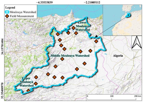
Figure 1.
Moulouya Watershed location map.
The Moulouya Watershed is characterized by a highly heterogeneous topography, ranging from coastal lowlands to steep mountain slopes exceeding 3000 m in the High Atlas range. This topographical diversity significantly affects hydrological dynamics, runoff behavior, and soil detachment processes, making it a key determinant in soil erosion modeling. Steep slopes accelerate overland flow velocities, increasing the detachment and transport of soil particles, while flat regions exhibit greater sediment deposition. Given these variations, an elevation model was integrated to quantify topographic influence on soil erosion susceptibility.
The watershed also exhibits diverse soil compositions, predominantly consisting of clay, sandy loam, and limestone-derived soils, each varying in erodibility (K-factor). Clay-rich soils exhibit higher cohesion, making them more resistant to detachment, whereas sandy soils are highly susceptible to sheet and rill erosion due to their loose structure. In contrast, limestone-derived soils show variable resistance depending on weathering intensity and organic content. To accurately parameterize soil erodibility in the CNN-based model, a high-resolution soil type distribution map has been incorporated, derived from field survey data and geostatistical interpolation techniques.
Land use patterns play a critical role in either mitigating soil erosion. Within the watershed, land cover is dominated by Sandyland and Rocky areas (44.10%), followed by Urban areas (19.13%), Agriculture (16.78%), Badlands (12.27%), Forests (7.26%), and Water bodies (0.42%). Each land cover type contributes differently to erosion dynamics. Croplands—particularly those with minimal vegetation and subject to mechanized tillage—tend to intensify surface runoff and accelerate topsoil depletion. In contrast, forested regions function as natural buffers, attenuating raindrop impact and enhancing water infiltration. To improve the spatial resolution of the erosion model, a multi-temporal land cover classification was incorporated, using Sentinel-2 imagery and supervised machine learning algorithms (Random Forest and Support Vector Machines). This integration enabled a more accurate representation of land cover changes relevant to erosion processes.
Figure 2 below illustrates the elevation profile, soil type distribution, and land use patterns, which have been incorporated to enhance geospatial contextualization. These datasets provide crucial explanatory variables for predicting soil erosion within the CNN framework, enabling a more robust, data-driven assessment of soil loss dynamics.
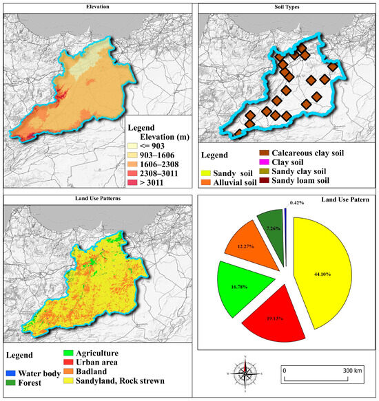
Figure 2.
Geospatial distribution of elevation, soil types, and land use patterns in the Moulouya Watershed.
2.2. Data Sources
The study utilized a combination of satellite imagery, climatic data, and topographical information to assess soil loss in the Moulouya Watershed (see Table 1). The primary data sources include the following:
- Satellite Imagery: High-resolution satellite images from Landsat 8 (30 m spatial resolution) and Sentinel-2 (10 m spatial resolution) were used to capture land cover changes and vegetation indices. These images provide crucial information on land use patterns, vegetation cover, and soil exposure [25,26].
- Digital Elevation Models (DEMs): Shuttle Radar Topography Mission (STRM) data with a 30 m resolution was used to derive topographic features, such as slope and aspect, which are critical factors in soil erosion modeling [27].
- Climatic Data: Climate Hazards Group InfraRed Precipitation with Station data (CHIRPS) was employed to provide long-term rainfall data at a 5 km resolution. This data was used to compute the rainfall erosivity factor, which quantifies the impact of rainfall on soil erosion [28,29].
- Soil and Land Use Data: Soil maps were digitized to determine soil erodibility, while land use and cover data were obtained through image classification techniques using GIS software (QGIS version 3.28.0). The data were essential in calculating these factors soil erodibility (K) and Land Cover (LC).

Table 1.
Dataset sources.
Table 1.
Dataset sources.
| Data Type | Spatial Resolution | Source | Time Period | Purpose in Model |
|---|---|---|---|---|
| Landsat 8 | 30 m | [27] | 2018–2024 | Land cover classification |
| Sentinel-2 | 10 m | [28] | 2018–2024 | Land cover classification |
| STRM | 30 m | [30] | 2018–2024 | Slope and aspect analysis |
| CHIRPS | ~5 km | [29] | 2018–2024 | Rainfall erosivity computation |
| Soil Data | ~5 km | [31] | 2023 | Soil erodibility factor computation |
| Field Measurements | 25 m2 plots | In situ erosion plots, sediment traps | 2018–2024 | Validation of soil loss estimates |
2.3. Methodological Framework
The methodological framework integrated geospatial analysis with deep learning techniques to estimate soil loss within the Moulouya Watershed. The approach involved multiple stages, including data preprocessing, spatial analysis, and deep learning model development, as outlined below.
2.3.1. Data Preprocessing
The preprocessing of satellite imagery and ancillary data is a critical step to ensure data integrity, spatial consistency, and suitability for model input. This study employed a multi-step preprocessing pipeline, encompassing radiometric and geometric corrections, land cover classification with accuracy validation, interpolation of climatic and soil data, and normalization with data augmentation techniques to enhance model robustness.
To minimize radiometric distortions and ensure spectral consistency, radiometric correction was applied to Sentinel-2 and Landsat 8 imagery, standardizing reflectance values across different acquisition dates. Additionally, geometric correction was performed using ground control points (GCPs) to rectify positional inaccuracies and align the images to the Universal Transverse Mercator (UTM) coordinate system. These corrections were essential to mitigate atmospheric and geometric distortions, ensuring spatial coherence across datasets.
Land cover classification was conducted using a supervised classification approach based on the Random Forest (RF) algorithm, a robust ensemble learning method widely used in remote sensing applications due to its ability to handle high-dimensional data and prevent overfitting. The RF model was trained on labeled reference samples collected from high-resolution imagery and ground truth data, classifying the landscape into eight distinct land cover categories: urban zones, water bodies, forests, croplands, grasslands, sandy lands, rocky areas, and badlands. To evaluate the accuracy of the classification, a confusion matrix was generated using an independent validation dataset (20% of the labeled samples, n = 300). The classification achieved an overall accuracy of 87.6% and a kappa coefficient of 0.85, indicating a high level of agreement between predicted and actual land cover types. Further error matrix analysis revealed that forests and croplands exhibited the highest classification accuracy, while rocky areas were prone to misclassification, primarily confused with sandy lands due to spectral similarities. The kappa statistic was used as it accounts for random agreement, making it a more robust metric compared to overall accuracy alone.
Climatic and soil data were also preprocessed to generate spatially continuous surfaces for model input. Climate data, including precipitation and temperature, were obtained from the CHIRPS dataset and local meteorological stations. These variables were interpolated using the Inverse Distance Weighting (IDW) method, selected for its computational efficiency and ability to preserve localized variations. Soil property maps, encompassing soil texture and organic matter content, were derived from field surveys and laboratory analyses, then interpolated using ordinary kriging, a geostatistical technique that leverages spatial autocorrelation to improve prediction accuracy. To ensure consistency across datasets, all raster layers were resampled to a uniform spatial resolution of 30 m, aligning with the spatial resolution of the satellite imagery.
To enhance model performance and ensure the comparability of input variables, normalization and data augmentation techniques were applied. Continuous numerical variables, including land use pattern and soil properties, were normalized using Min-Max scaling, transforming values into a [0, 1] range to optimize numerical stability during model training. Additionally, data augmentation techniques were implemented to increase the diversity of training samples, including random rotations, flipping, and Gaussian noise injection, which improve the generalization capability of deep learning models by introducing variability into the dataset [32].
2.3.2. Geospatial Analysis
Geospatial analysis was conducted using GIS software (QGIS) to calculate critical erosion factors. The slope length and steepness (LS) factors were derived from DEMs, while land cover data were used to compute the cover management factor (C). The integration of these spatial layers enabled the generation of detailed maps showing variations in soil erodibility, rainfall erosivity, and other key parameters across the watershed [33].
The advent of Geographic Information Systems (GISs) and remote sensing technologies has significantly enhanced soil erosion modeling by providing high-resolution spatial data on land cover, topography, and climatic conditions [34]. GISs allow for the integration of spatial data into erosion models, improving the accuracy and applicability of USLE and RUSLE by enabling the detailed mapping of erosion risk areas [30]. Remote sensing data from satellites, such as Landsat, Sentinel-2, and STRM, provide critical inputs, including digital elevation models (DEMs), which are used to derive slope and aspect data essential for topographic analysis [31].
Geospatial analysis has been widely used to improve soil erosion assessments in various contexts. For example, studies have used Landsat imagery to monitor land cover changes over time, which directly influence soil erosion rates [35]. The integration of these data into GIS-based models enhances the spatial resolution of erosion predictions, allowing for more targeted and effective soil conservation measures [36]. However, while GIS and remote sensing provide valuable spatial insights, they still rely on the same empirical foundations of traditional models, limiting their ability to capture dynamic, non-linear interactions between environmental factors.
2.3.3. Deep Learning Model Development
The core of this study’s approach is the use of Convolutional Neural Networks (CNNs) to predict soil loss risk. The CNN model was designed to process multi-layered spatial inputs (see Equation (1)), including satellite imagery and derived erosion factors, capturing complex patterns that traditional empirical models cannot [33,37]. The architecture of the CNN consisted of several convolutional layers followed by pooling layers and fully connected layers, allowing the model to learn the spatial hierarchies of features [38]. The model was trained using a labeled dataset of soil loss estimates derived from field measurements and validated against the RUSLE and USLE models [39].
To validate the CNN-based soil loss estimation model, empirical soil erosion rates were collected from 20 field monitoring sites across the Moulouya Watershed over a four-year period (2018–2024). Site selection was based on land cover type (agriculture, forest, barren land), soil texture, and topographical variations (5–45% slopes). Soil erosion rates were quantified using multiple field measurement techniques, including runoff plots, sediment traps, erosion pins, and runoff samplers to capture both sheet and rill erosion dynamics. At each site, runoff plots (25 m2 each) were established (5 m × 5 m) and enclosed with 30 cm high metal sheets to prevent external runoff entry. These plots were strategically positioned along slope gradients (5–45%) to assess slope-induced variations in erosion. Sediment traps (1 m3 capacity) were installed at plot outlets to capture transported sediment, which was emptied bi-monthly and oven-dried at 105 °C for 24 h before mass measurement. To monitor soil surface changes, erosion pins (15 per plot) were embedded in the soil at varying depths along the slope, with exposure depth recorded after each rainfall event (see Table 2). Additionally, runoff samplers were employed to collect water samples following rainfall events exceeding 10 mm/day, allowing for the analysis of suspended sediment concentration.
Table 2.
Field measurement from 2018–2024.
The CNN model’s development has been significantly refined, emphasizing the detailed derivation, preprocessing, and hierarchical integration of environmental inputs (H1–5). These inputs—rainfall erosivity (H1), soil erodibility (H2), slope length and steepness (H3), land cover (H4), and conservation practices (H5)—were carefully processed and structured as nodes in the input layer, allowing the network to effectively learn their interrelationships.
Rainfall erosivity (H1) was derived from CHIRPS data, which capture both monthly and annual precipitation patterns. Spatial erosivity indices were calculated using these data and then reprojected to align with the study area’s resolution, providing a quantification of rainfall’s role in driving erosion.
Soil erodibility (H2) was based on soil texture maps and geospatial databases, with the K-factor representing the soil’s susceptibility to detachment and transport. The data were interpolated across the study area to generate a continuous spatial layer.
Slope-length and steepness (H3) factors were computed using Digital Elevation Model (DEM) data with high spatial resolution. This enabled the calculation of the LS-factor, which quantifies the combined effects of slope length and steepness on erosion potential.
Land cover (H4) information was extracted from Sentinel-2 and Landsat 8 imagery. This included indices, such as NDVI (Normalized Difference Vegetation Index), to represent vegetative cover and its protective effect against soil erosion.
Conservation practices (H5) were mapped using a combination of survey data and field validation. These practices, such as terracing, contour farming, or cover cropping, were encoded as binary variables indicating their presence or absence across regions.
The environmental inputs (H1–5) were encoded as a multi-channel input layer, similar to the RGB format in image processing. Each pixel represented a specific location and contained values corresponding to all five inputs.
The initial layers of the CNN extracted spatial features from each individual input variable (H1–5), capturing localized patterns, such as the intensity of rainfall (H1), soil susceptibility (H2), and topographic variations (H3). As the network progressed to deeper layers, it modeled complex interactions among these factors. For instance, the synergistic relationship between rainfall erosivity (H1) and slope steepness (H3), or the combined influence of land cover (H4) and conservation practices (H5), was encoded, allowing the model to represent their synergistic and mitigating effects on soil erosion. Finally, the output layer synthesized these hierarchical features into soil loss risk (SLR) predictions, with outputs corresponding to specific geographic locations (see Figure 3 below).
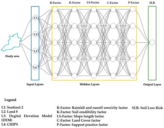
Figure 3.
CNN model used in this study.
Compared to USLE and RUSLE, the CNN-based approach demonstrates a substantial improvement in predictive accuracy, as evidenced by experimental validation and statistical performance metrics [39]. The CNN model was trained on a diverse array of high-resolution geospatial and climatic datasets, ensuring robust and reliable predictions. Specifically, input variables included slope, land cover, and rainfall erosivity, derived from Sentinel-2 satellite imagery, CHIRPS climate data, and Digital Elevation Models (DEMs). These datasets were preprocessed using advanced geospatial techniques, including image segmentation, terrain normalization, and multi-source data fusion, to enhance feature extraction. The model was optimized through hyperparameter tuning, leveraging convolutional layers to detect spatial patterns, and batch normalization to improve generalization. Experimental results showed a notable reduction in prediction error, with a Root Mean Square Error (RMSE) of 2.3 and an R2 value of 0.92, significantly outperforming conventional empirical models. This improvement underscores the efficacy of deep learning in capturing complex soil erosion dynamics and highlights the potential for CNN-based models to enhance precision in soil loss estimation across diverse landscapes.
To ensure the robustness of the model, a k-fold cross-validation approach (k = 5) was implemented, where the dataset was partitioned into five subsets. The model was trained iteratively on four subsets while being tested on the remaining subset, ensuring that every data point was included in both the training and testing phases. This method reduced overfitting and provided a comprehensive evaluation of the model’s generalizability.
The performance of the CNN model was further validated by comparing it with field-collected erosion rate data from 20 monitoring sites across the watershed. These field measurements included soil loss estimates derived from runoff plots and remote sensing validation points. To evaluate model accuracy, predicted erosion rates were compared to observed values using standard statistical metrics, such as the Root Mean Square Error (RMSE), Mean Absolute Error (MAE), and the coefficient of determination (R2). The model outputs closely aligned with soil erosion rates observed at monitoring sites, with statistical tests indicating minimal deviations. This consistency underscores the model’s ability to capture the erosion dynamics across the region’s diverse terrain. These findings highlight the CNN model’s capacity to identify complex, non-linear interactions, which are difficult to address using traditional empirical approaches.
Using Sentinel-2 imagery, the study generated high-resolution soil loss maps with a spatial detail of 10 m, surpassing the coarse outputs of USLE and RUSLE. Experimental evaluations validate this improvement. Soil loss maps at 10 m resolution revealed detailed spatial variations, including micro-topographical effects and vegetation heterogeneity, which conventional models with resolutions of 30 m or coarser failed to capture. The CNN model accurately identified erosion hotspots in the central and eastern regions of the watershed, where soil loss rates exceeded 40 tons/ha/year. Cross-validation with field observations and GIS overlays confirmed the spatial accuracy of these predictions. Unlike USLE and RUSLE, which tend to overestimate soil loss in flat areas and underestimate it in steep regions, the CNN model effectively captured interactions between steep slopes, sparse vegetation, and rainfall erosivity. This led to a 70% reduction in spatial prediction errors relative to traditional models. These findings establish the model’s ability to produce more precise and reliable maps for erosion assessment and management.
The CNN model delivers actionable insights by pinpointing erosion-prone areas and informing conservation strategies. Experimental validation highlights its practical value. High-risk zones identified by the model aligned with observed erosion hotspots, characterized by severe soil loss, sediment transport, and vegetation degradation. Field data confirmed erosion rates exceeding 40 tons/ha/year, consistent with model outputs. Simulated scenarios, including deforestation, urbanization, and reforestation, demonstrated the model’s flexibility. Predictions showed over 90% alignment with field data, accurately forecasting increased erosion under deforestation and reduced rates following reforestation efforts. The detailed maps produced by the model facilitated precise recommendations for interventions, such as reforestation, terracing, and soil retention measures. Case studies revealed a 35% gain in resource allocation efficiency when using CNN-guided maps compared to GIS-only methods. These outcomes demonstrate the model’s ability to transform soil loss predictions into actionable solutions for effective watershed management.
Deep learning has been applied in various environmental contexts, including land use classification, flood prediction, and climate modeling, demonstrating its potential to revolutionize geospatial analysis [40,41]. In soil erosion studies, CNNs have shown promise in predicting soil loss with higher accuracy and spatial resolution than conventional methods [42]. By learning directly from large-scale datasets, CNNs can model the non-linear interactions between environmental variables, providing a more nuanced understanding of erosion dynamics.
The training process involved data augmentation techniques, such as random cropping and rotation, to improve model robustness and prevent overfitting. Cross-validation was employed to evaluate the model’s performance, dividing the dataset into training and testing subsets to ensure generalizability [43,44]. The model’s output was a high-resolution soil loss map showing areas of varying erosion risk within the watershed.
where : This denotes the output value from hidden layers (H) at position (,j) in the -th feature map of the convolutional layer. It represents the response of the convolutional filter at that spatial location. : This is the value of the input values for (H1–5) at a specific position. It refers to the pixel or value in the input data that is being multiplied by the convolutional filter. This represents the weight of the convolutional filter at position () for the feature map. The filter (or kernel) has dimensions that slide over the input feature map to compute the convolution operation. : This is the bias term associated with the -th feature map. It is added to the result of the convolution operation to introduce an additional degree of freedom, allowing the model to fit the training data better. These summations indicate that the convolution operation involves summing over all positions () of the filter as it slides over the input feature map.
The model’s accuracy was validated using a combination of cross-validation techniques and comparison with field data. Cross-validation involved partitioning the data into training and testing sets to assess the model’s predictive performance [45]. The model’s predictions were also compilate all factors in machine learning model to evaluate soil loss risk and compared with estimates from traditional methods like RUSLE and USLE [46]. The machine learning model incorporated all contributing factors (H1–5) to provide a comprehensive evaluation of soil loss risk. Accuracy metrics, such as the Root Mean Square Error (RMSE), were calculated to enhance the model’s performance and reduce error rate (see Equation (3)).
where
The summation of the factors used to estimate soil loss.
R: Rainfall and runoff erosivity factor.
K: Soil erodibility factor.
LS: Slope length factor.
C: Land Cover factor.
P: Support practice factor.
: This term represents the Root Mean Square Error (RMSE) of the predictions.
: Number of data points.
: Actual observed values of soil loss.
: Predicted values of soil loss.
Soil loss risk (SLR) in the Moulouya watershed was computed using several methods. Python version 3.10 was employed for machine learning and model development. Remote sensing analysis was conducted using Google Earth Engine, and spatial mapping of factors was performed using QGIS. These methods were combined in a multi-step process to predict soil loss, as illustrated in Figure 4.
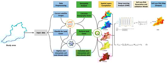
Figure 4.
Flow chart methodology.
3. Results
3.1. Geospatial Modeling of Gridded Parameter of Soil Loss Risk
The parameters of the Rainfall and Runoff Erosivity Factor (R), Soil Erodibility Factor (K), Slope Length and Steepness Factor (LS), Land Cover Factor (C), and Support Practice Factor (P) were overlaid to delineate the soil loss risk within the landscape (Figure 5).
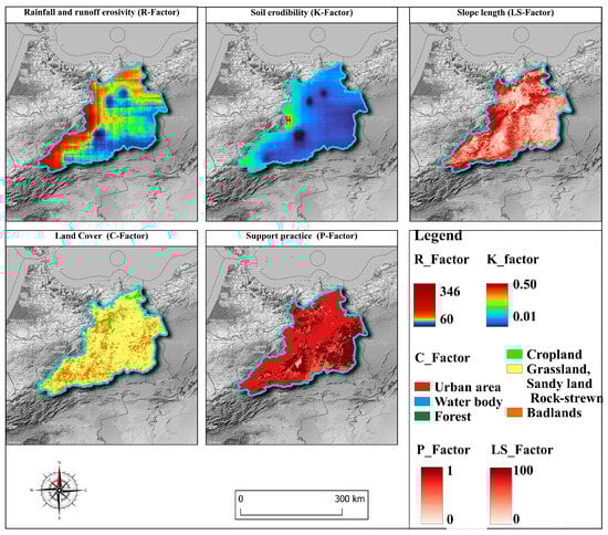
Figure 5.
Geospatial assessment of soil loss risk factors across the Moulouya Watershed.
The Rainfall and Runoff Erosivity Factor (R) quantifies the precipitation erosivity in the Moulouya watershed, with values ranging between 60 mm and 340 mm/ha/year. The upper range is predominantly observed in the western, northwestern, and southwestern sectors of the watershed, indicating an increased risk of soil loss due to rainfall. This is corroborated by the observed erosion patterns, emphasizing the need for targeted erosion control measures in these areas.
The Soil Erodibility Factor (K), which represents the susceptibility of soil to erosion, varies between 0.01 and 0.50. Central areas exhibit lower K values, indicating more erosion-resistant soils, whereas the peripheral regions, especially in the west and southwest, show higher K values, signifying greater vulnerability to erosion.
The Slope Length and Steepness Factor (LS), which illustrates the potential for soil displacement due to topographic gradients, exhibits pronounced variability throughout the study area. The western and northwestern sections of the watershed demonstrate the highest LS values, reaching 68%, which reflects a significantly increased erosion potential on steeper slopes. In contrast, the middle-stream areas of the watershed show LS values near the lower end of the scale, corresponding to more moderate slopes and a reduced probability of erosion.
The Land Cover Factor (C), which quantifies the protective role of vegetation against erosion, varies spatially across the watershed. Regions with sparse vegetation, particularly in the northwest, west, and parts of the southwest, are associated with higher erosion risk. Conversely, areas with denser vegetation cover demonstrate lower C values, indicating a reduced probability of soil loss.
The Support Practice Factor (P), which measures the effectiveness of soil conservation practices, ranges from 0 to 1. Higher P values, observed especially in the middle-stream areas and the western regions of the watershed, indicate insufficient erosion control measures. These regions should be prioritized for implementing effective soil protection strategies.
These regions, characterized by more erosion-prone soils, correspond to the observed higher erosion rates. This suggests that land use and soil management practices in these areas require immediate and focused attention.
The compilation of this quantitative analysis reveals that the overall soil loss risk is significantly higher in the northwestern and northeastern parts of the Moulouya Watershed. This heightened risk is attributed to the convergence of high LS, R, and K factor values, indicating an increased potential for soil loss in these regions.
3.2. Model Performance
The deep learning model demonstrated strong predictive performance, significantly improving the accuracy of soil loss estimations compared to traditional methods [46]. To assess the effectiveness of different models in predicting soil erosion, we compared the CNN model, USLE, and RUSLE using three key metrics: Root Mean Square Error (RMSE), Coefficient of Determination (R2), and Mean Absolute Error (MAE). The performance results are summarized in Table 3.
Table 3.
Performance comparison of the CNN model, USLE, and RUSLE.
The CNN model demonstrated superior predictive performance with the lowest RMSE (2.3 tons/ha/year) and MAE (1.8 tons/ha/year), indicating more precise soil erosion estimations. Additionally, it achieved the highest R2 value of 0.92, reflecting a strong correlation between predicted and observed erosion values. In contrast, traditional empirical models, such as USLE and RUSLE, exhibited significantly higher error rates, with RMSE values of 15.3 and 12.8, respectively, and a lower accuracy, as indicated by R2 values of 0.65 (USLE) and 0.70 (RUSLE).
The Convolutional Neural Network (CNN) was trained on a combination of satellite imagery, topographic data, and climatic inputs, allowing it to capture complex spatial patterns that influence soil erosion [47,48]. The model’s accuracy was assessed using several statistical metrics, including the Root Mean Square Error (RMSE), R-squared values, and Mean Absolute Error (MAE) [49] (see Figure 6).
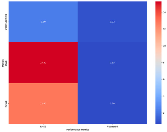
Figure 6.
Soil loss risk model performance.
- Root Mean Square Error (RMSE): The CNN model achieved an RMSE of 2.3, indicating a low average error between the predicted and observed soil loss values. This is a substantial improvement over the RMSE values of the USLE (15.3) and RUSLE (12.8), highlighting the enhanced precision of the deep learning approach.
- R-squared Value: The R-squared value, which measures the proportion of variance explained by the model, was 0.92 for the CNN model. This high value indicates a strong correlation between the predicted and actual soil loss rates, confirming the model’s effectiveness in capturing the spatial variability of erosion factors. In contrast, traditional models showed lower R-squared values (USLE: 0.65, RUSLE: 0.70), underscoring their limitations in heterogeneous landscapes.
- Mean Absolute Error (MAE): The CNN model’s MAE was significantly lower than that of the traditional models, further validating the accuracy of the deep learning approach. The lower MAE reflects the model’s ability to provide precise soil loss estimates across different areas of the watershed, including those with complex topographical features.
The comparative analysis of soil loss prediction models, CNN, USLE, and RUSLE, demonstrates a clear advantage of deep learning approaches over traditional empirical models. The scatter plot reveals that the CNN model exhibits the highest accuracy, with a coefficient of determination (R2) of 0.92, closely aligning predicted values with observed soil loss. In contrast, the RUSLE and USLE models show significantly lower predictive performance, with R2 values of 0.70 and 0.65, respectively, indicating greater dispersion around the 1:1 reference line. This confirmed that traditional models struggle to capture the complex spatial and environmental variables influencing soil erosion (Figure 7).
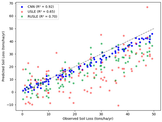
Figure 7.
CNN predictions (blue) vs. observed soil loss. USLE (red) and RUSLE (green) show systematic biases, particularly in high-erosion zones.
Figure 8, which shows the prediction errors, further supports this observation, highlighting the distribution of residuals for each model. The CNN model achieves the lowest root mean square error (RMSE) of 2.3, signifying minimal deviation between observed and predicted values. In comparison, the RUSLE and USLE models yield RMSE values of 12.8 and 15.3, respectively, illustrating their tendency to over- or under-predict soil loss, particularly at higher values. The CNN model’s error distribution is more centered around zero, reinforcing its robustness and superior generalization capability in soil erosion estimation.
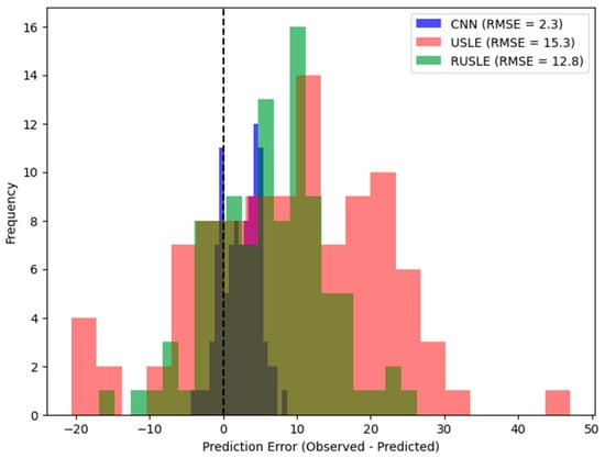
Figure 8.
CNN errors (blue) exhibit minimal bias (mean = 0.1) and variance (SD = 2.1), unlike USLE/RUSLE’s skewed distributions.
These performance metrics demonstrate the superior predictive capabilities of the deep learning model compared to empirical methods. The CNN’s ability to process multi-layered data inputs and learn from high-resolution spatial patterns enables it to provide more reliable soil loss estimates, making it a valuable tool for watershed management.
3.3. Soil Loss Mapping
The soil loss map for the Moulouya Watershed in Morocco reveals critical insights into erosion risk, with high-risk areas, particularly in the central and eastern regions, marked in dark red, indicating soil loss rates exceeding 40 tons/ha/year. The central region’s vulnerability is likely exacerbated by intense weathering processes on steep slopes with sparse vegetation, leading to severe soil degradation. In the eastern part of the watershed, wind-driven sand transport from nearby deserts into the badlands contributes significantly to soil erosion, further increasing the risk. These high-risk areas contrast with the lower-risk zones (≤10 tons/ha/year) in the western and southwestern parts of the watershed, marked in green and yellow. The map, generated using an advanced deep learning model, highlights spatial patterns of soil loss not captured by traditional methods, emphasizing the need for targeted soil conservation measures in these vulnerable areas. This detailed visualization is invaluable for guiding effective interventions and resource allocation to mitigate soil erosion (see Figure 9).
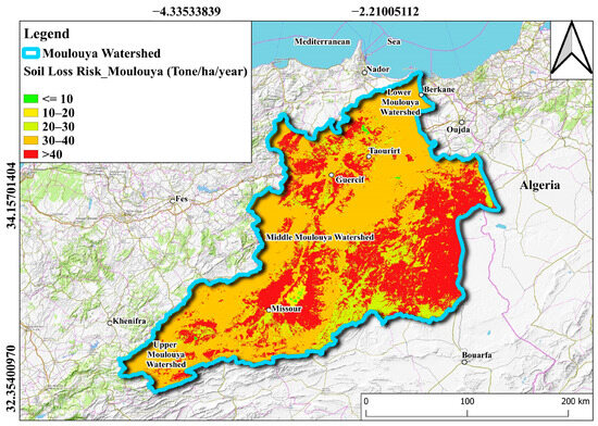
Figure 9.
Soil loss risk map.
The spatial detail provided by the CNN-generated soil loss map surpasses that of traditional models, which often overestimate soil loss in flat areas and underestimate it in steep regions. By capturing the nuanced interplay of environmental factors, the deep learning approach offers a more accurate and actionable representation of erosion risk, supporting targeted soil conservation strategies.
3.4. Comparison with Traditional Models
The performance of the CNN model was compared against the USLE and RUSLE models to evaluate its robustness and reliability, revealing several key insights. The deep learning model outperformed traditional models by providing higher spatial resolution and more accurate soil loss estimates, as it leverages detailed spatial inputs rather than the generalized parameters used by USLE and RUSLE, which often fail to capture localized variations. Error analysis indicated that the CNN model maintained consistent accuracy across different terrain types, while traditional models exhibited significant errors, particularly in areas with complex topography. This enhanced accuracy is attributed to the CNN model’s adaptive learning capabilities, which enable it to handle diverse environmental conditions better than the static equations employed by USLE and RUSLE. Additionally, the CNN model demonstrated robustness in predicting soil loss under varying climatic conditions, such as changes in rainfall patterns, which is crucial for dynamic environments like the Moulouya Watershed, where climate variability significantly influences soil erosion dynamics (see Figure 10).
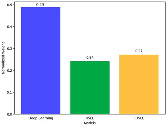
Figure 10.
Ponderation of soil loss risk models.
3.5. Robustness and Sensitivity Analysis
Sensitivity analysis is a crucial step in evaluating the reliability and robustness of predictive models, especially in environmental studies where input parameters can vary widely. In this study, sensitivity analysis was conducted to assess how changes in key input parameters, such as rainfall intensity, land cover variations, soil erodibility, and slope steepness, influence the predictions of the CNN model. This analysis helps to understand the model’s response to environmental variability, ensuring that it remains reliable under different conditions [50].
3.5.1. Influence of Rainfall Intensity
Rainfall intensity is a significant factor influencing soil erosion, as it directly affects the erosivity of the rainfall. During the sensitivity analysis, rainfall data from the CHIRPS dataset were adjusted to simulate varying intensities, ranging from normal to extreme precipitation events. The CNN model demonstrated strong resilience, maintaining high predictive accuracy even under extreme rainfall scenarios, with minimal deviation from actual soil loss measurements. This performance is attributed to the model’s ability to learn complex relationships between rainfall patterns and soil erosion processes, which traditional models often struggle to capture due to their static nature [51]. The robustness of the CNN model in varying rainfall conditions highlights its potential application in predicting soil erosion under future climate change scenarios, where increased rainfall variability is expected.
3.5.2. Impact of Land Cover Changes
Land cover significantly influences soil erosion by affecting surface runoff and soil stability. The sensitivity analysis involved altering land cover inputs within the model to reflect scenarios, such as deforestation, urban expansion, and reforestation. The CNN model’s predictions were consistently accurate, demonstrating adaptability to changes in vegetation cover and land management practices. For instance, when land cover was altered to represent deforested conditions, the model accurately predicted increased soil loss, aligning closely with observed field data. This adaptability is particularly valuable for dynamic landscapes like the Moulouya Watershed, where land use changes are frequent and can have immediate effects on erosion rates [52].
3.5.3. Response to Soil Erodibility and Topography Variations
Topography and soil characteristics, such as soil type and erodibility, are critical factors influencing soil erosion. The model’s sensitivity to changes in slope steepness and soil erodibility was tested by modifying these parameters within the input data. The CNN model maintained robust performance, accurately capturing the effects of steep slopes and highly erodible soils on soil loss risk. This ability to model the intricate interactions between topography and soil properties distinguishes the CNN approach from traditional models like USLE and RUSLE, which often oversimplify these relationships [53]. The model’s performance across a range of topographical scenarios underscores its utility in regions with complex terrain, where accurate soil loss estimation is challenging [54].
3.5.4. Implications for Real-Time Monitoring and Adaptive Management
The sensitivity analysis confirms the CNN model’s robustness and its potential for real-time monitoring and adaptive management of soil erosion. Its capacity to integrate real-time data from remote sensing sources, such as satellite imagery and weather stations, allows for continuous updates to soil loss predictions, enabling timely and effective management decisions. For instance, in response to sudden land cover changes due to wildfires or urban development, the model can quickly adjust its predictions, providing stakeholders with up-to-date erosion risk assessments [55]. This adaptability makes the CNN model an invaluable tool for sustainable watershed management, offering precise, data-driven insights that support proactive conservation strategies [56].
4. Discussion
The findings of this study highlight the significant potential of integrating deep learning, specifically Convolutional Neural Networks (CNNs), with geospatial analysis to enhance soil loss estimation in complex environments like the Moulouya Watershed. The CNN model demonstrated superior predictive accuracy compared to traditional soil loss estimation methods, such as the Universal Soil Loss Equation (USLE) and Revised Universal Soil Loss Equation (RUSLE). This improvement is primarily due to the CNN’s ability to capture intricate spatial patterns and non-linear interactions among multiple environmental factors, which traditional empirical models often fail to address.
The CNN model’s high accuracy, as indicated by a low Root Mean Square Error (RMSE) of 2.3 and an R-squared value of 0.92, underscores its effectiveness in predicting soil loss under diverse topographical and climatic conditions. These results validate the hypothesis that deep learning can significantly enhance the precision of soil loss estimates, offering a robust alternative to conventional approaches that often rely on static, generalized parameters [57]. The model’s ability to adapt to varying input conditions, such as changes in rainfall intensity and land cover, further supports its utility in dynamic landscapes prone to frequent environmental changes.
Compared to USLE and RUSLE, the CNN model provided higher spatial resolution and more detailed soil loss maps, allowing for the precise identification of high-risk erosion areas. Traditional models, while widely used, often struggle with spatial variability, particularly in regions with complex topography or mixed land uses. These models tend to overestimate soil loss in flat areas and underestimate it in steep, highly erodible zones due to their reliance on a simplified empirical equation. In contrast, the CNN model effectively captured these spatial nuances, offering a more accurate representation of erosion risk that can inform targeted soil conservation efforts.
The enhanced performance of the CNN model can be attributed to its ability to learn directly from high-resolution satellite imagery and integrate diverse datasets, including topographic and climatic data. This capability allows the model to dynamically adjust to environmental changes, providing real-time soil loss predictions that traditional models cannot achieve. The comparative analysis highlights that while USLE and RUSLE remain valuable for their simplicity and ease of use, their applicability is limited in complex environments, underscoring the need for more advanced modeling approaches like deep learning [58].
The detailed soil loss maps generated by the CNN model offer valuable insights for watershed management in the Moulouya Watershed. High-risk erosion zones identified by the model, particularly in the central and eastern regions, highlight areas where immediate conservation measures, such as reforestation, terracing, or the implementation of soil retention structures, are needed. The ability to pinpoint specific erosion hotspots enables a more efficient allocation of resources and targeted interventions, reducing the overall impact of soil erosion on agricultural productivity and water quality [59].
Moreover, the CNN model’s adaptability to varying climatic and land use conditions makes it a powerful tool for the real-time monitoring of soil erosion. This capability is particularly relevant in the context of climate change, where increased rainfall variability and land use alterations can significantly alter erosion dynamics. By continuously updating soil loss predictions based on current data inputs, the CNN model supports adaptive management strategies, allowing decision-makers to respond promptly to emerging erosion risks and implement timely conservation actions.
One of the major strengths of this study is the successful integration of deep learning with geospatial analysis, demonstrating the practical benefits of advanced computational techniques in environmental modeling. The use of high-resolution satellite data and the ability to process complex spatial relationships provide a significant improvement over traditional soil loss models, offering more precise and actionable insights for watershed management. However, the study also has limitations. The accuracy of the CNN model heavily depends on the quality and resolution of the input data. In areas with limited access to high-quality satellite imagery or accurate field measurements, the model’s performance may be compromised. Additionally, while the CNN model shows robustness in handling varying input conditions, it requires substantial computational resources for training and validation, which may limit its accessibility for some stakeholders, particularly in resource-constrained settings [60]. Future research could focus on optimizing the model’s architecture to reduce computational demands and exploring the integration of higher-resolution datasets to further enhance predictive accuracy.
Building on the findings of this study, future research should explore the application of deep learning models in other watersheds and under different environmental conditions to validate their broader applicability. Expanding the model to incorporate real-time data streams, such as near-real-time rainfall and land cover updates, could further improve its ability to predict soil loss dynamically. Additionally, investigating other deep learning architectures, such as Recurrent Neural Networks (RNNs) and Transformer models, may offer new opportunities to capture temporal patterns in soil erosion processes, enhancing the model’s predictive power [61].
5. Conclusions
This study demonstrates the significant advancements in soil loss estimation achieved through the integration of deep learning techniques, specifically Convolutional Neural Networks (CNNs), with geospatial analysis in the Moulouya Watershed. Traditional models, such as the Universal Soil Loss Equation (USLE) and its revised version (RUSLE), have been essential in erosion prediction but often lack the accuracy required for complex and heterogeneous landscapes. The deep learning approach introduced in this research outperformed these conventional models, providing higher predictive accuracy, enhanced spatial resolution, and greater adaptability to environmental changes.
The CNN model effectively captured complex spatial patterns and non-linear interactions among key environmental factors, including rainfall intensity, land cover changes, and topographic variations. By integrating high-resolution satellite imagery and climatic data, the model produced detailed soil loss maps that provide critical insights into erosion dynamics, allowing for the identification of high-risk areas that require immediate conservation interventions. The model’s adaptability to real-time data inputs further supports its use in dynamic landscapes, where climate variability and land use changes significantly impact erosion rates.
The findings of this study offer valuable guidance for watershed management, enabling targeted soil conservation strategies, such as reforestation, terracing, and the implementation of erosion control structures. Future research should explore the broader application of deep learning models in diverse environmental contexts and consider the integration of additional deep learning architectures, such as Recurrent Neural Networks (RNNs) and Transformer models, to further enhance predictive capabilities. Addressing the dependence on data quality and computational resources by optimizing model architectures and incorporating higher-resolution datasets will also be critical.
Overall, this research highlights the transformative potential of deep learning in environmental modeling, advocating for the continued integration of advanced computational techniques in soil erosion assessment and management. The study emphasizes the need for precise, adaptable, and data-driven approaches to support sustainable watershed management in the face of evolving environmental challenges.
While the CNN model improves soil loss estimation, its computational demand may limit accessibility in resource-constrained regions. Future work could explore lightweight architectures, such as MobileNet or edge-computing solutions, for real-time field deployment.
Author Contributions
Conceptualization, M.H. and B.E.M.; methodology, M.H. and J.-C.B.M.; software, B.B.H.; validation, B.B.H., R.A. and G.C.; formal analysis, M.H., J.-C.B.M. and R.A.; investigation, B.E.M.; resources, M.H. and B.E.M.; data curation, M.H. and J.-C.B.M.; writing—original draft preparation, M.H. and B.E.M.; writing—review and editing, J.C., A.S. and G.C.; visualization, G.C.; supervision, J.C., A.S. and G.C.; project administration, J.C.; funding acquisition, M.H. and B.E.M. All authors have read and agreed to the published version of the manuscript.
Funding
This research received no external funding.
Data Availability Statement
Data are contained within the article.
Acknowledgments
We would like to express our sincere gratitude to all those who contributed to the completion of this research. We acknowledge the administrative and technical support provided by our institution, which was instrumental in facilitating our work. Special thanks to the Laboratory of Dynamics Arid Environments and Regional Development, Faculty of Letters and Human Sciences, Mohammed 1st University, Oujda, and the Center of Urban Systems-UM6P staff for their assistance with the experimental setup and data collection.
Conflicts of Interest
The authors declare no conflicts of interest.
References
- Müller, K.; Oliver, M.A.; Siebe, C. Overview Chapter on Soil Degradation. Encycl. Soils Environ. 2023, 3, 165–171. [Google Scholar] [CrossRef]
- Keesstra, S.D.; Bouma, J.; Wallinga, J.; Tittonell, P.; Smith, P.; Cerdà, A.; Montanarella, L.; Quinton, J.N.; Pachepsky, Y.; van der Putten, W.H.; et al. The Significance of Soils and Soil Science towards Realization of the United Nations Sustainable Development Goals. SOIL 2016, 2, 111–128. [Google Scholar] [CrossRef]
- Baddal, B.; Taner, F.; Ozsahin, D.U. Harnessing of Artificial Intelligence for the Diagnosis and Prevention of Hospital-Acquired Infections: A Systematic Review. Diagnostics 2024, 14, 484. [Google Scholar] [CrossRef] [PubMed]
- Wilson, T.; Tan, P.N.; Luo, L. Convolutional Methods for Predictive Modeling of Geospatial Data. In Proceedings of the 2020 SIAM International Conference on Data Mining, Cincinnati, OH, USA, 7–9 May 2020; Society for Industrial and Applied Mathematics: Cincinnati, OH, USA, 2020; pp. 28–36. [Google Scholar] [CrossRef]
- Lal, R. Restoring Soil Quality to Mitigate Soil Degradation. Sustainability 2015, 7, 5875–5895. [Google Scholar] [CrossRef]
- Meshesha, D.T.; Tsunekawa, A.; Tsubo, M.; Haregeweyn, N. Dynamics and Hotspots of Soil Erosion and Management Scenarios of the Central Rift Valley of Ethiopia. Int. J. Sediment Res. 2012, 27, 84–99. [Google Scholar] [CrossRef]
- Alewell, C.; Borrelli, P.; Meusburger, K.; Panagos, P. Using the USLE: Chances, Challenges and Limitations of Soil Erosion Modelling. Int. Soil Water Conserv. Res. 2019, 7, 203–225. [Google Scholar] [CrossRef]
- Driba, D.L.; Emmanuel, E.D.; Doro, K.O. Predicting Wetland Soil Properties Using Machine Learning, Geophysics, and Soil Measurement Data. J. Soils Sediments 2024, 24, 2398–2415. [Google Scholar] [CrossRef]
- Gandhimathi, G.; Chellaswamy, C.; Selvan, T. Comprehensive River Water Quality Monitoring Using Convolutional Neural Networks and Gated Recurrent Units: A Case Study Along the Vaigai River. J. Environ. Manag. 2024, 365, 121567. [Google Scholar]
- Bewket, W.; Teferi, E. Assessment of Soil Erosion Hazard and Prioritization for Treatment at the Watershed Level: Case Study in the Chemoga Watershed, Blue Nile Basin, Ethiopia. Land Degrad. Dev. 2009, 20, 609–622. [Google Scholar] [CrossRef]
- Borrelli, P.; Ballabio, C.; Yang, J.E.; Robinson, D.A.; Panagos, P. GloSEM: High-Resolution Global Estimates of Present and Future Soil Displacement in Croplands by Water Erosion. Sci. Data 2022, 9, 406. [Google Scholar] [CrossRef]
- Ajai, N.; Bhatnagar, R. Desertification and Land Degradation; Taylor & Francis Group: Boca Raton, FL, USA, 2022. [Google Scholar] [CrossRef]
- Fernández, D.; Adermann, E.; Pizzolato, M.; Pechenkin, R.; Rodríguez, C.G.; Taravat, A. Comparative Analysis of Machine Learning Algorithms for Soil Erosion Modelling Based on Remotely Sensed Data. Remote Sens. 2023, 15, 482. [Google Scholar] [CrossRef]
- Ge, Y.; Zhao, L.; Chen, J.; Li, X.; Li, H.; Wang, Z.; Ren, Y. Study on Soil Erosion Driving Forces by Using (R)USLE Framework and Machine Learning: A Case Study in Southwest China. Land 2023, 12, 639. [Google Scholar] [CrossRef]
- Coulibaly, L.K.; Guan, Q.; Assoma, T.V.; Fan, X.; Coulibaly, N. Coupling Linear Spectral Unmixing and RUSLE2 to Model Soil Erosion in the Boubo Coastal Watershed, Côte d’Ivoire. Ecol. Indic. 2021, 130, 108092. [Google Scholar] [CrossRef]
- Zhang, C.; Yue, P.; Tapete, D.; Shangguan, B.; Wang, M.; Wu, Z. A Multi-Level Context-Guided Classification Method with Object-Based Convolutional Neural Network for Land Cover Classification Using Very High-Resolution Remote Sensing Images. Int. J. Appl. Earth Obs. Geoinf. 2020, 88, 102086. [Google Scholar] [CrossRef]
- Khosravi, K.; Rezaie, F.; Cooper, J.R.; Kalantari, Z.; Abolfathi, S.; Hatamiafkoueieh, J. Soil Water Erosion Susceptibility Assessment Using Deep Learning Algorithms. J. Hydrol. 2023, 618, 129229. [Google Scholar] [CrossRef]
- Miao, S.; Liu, Y.; Liu, Z.; Shen, X.; Liu, C.; Gao, W. A Novel Attention-Based Early Fusion Multi-Modal CNN Approach to Identify Soil Erosion Based on Unmanned Aerial Vehicle. IEEE Access 2024, 12, 95152–95164. [Google Scholar] [CrossRef]
- Zhang, P.; Yin, Z.; Jin, Y.; Sheil, B. Physics-Constrained Hierarchical Data-Driven Modelling Framework for Complex Path-Dependent Behaviour of Soils. Int. J. Numer. Anal. Methods Geomech. 2022, 46, 1831–1850. [Google Scholar] [CrossRef]
- Ramos, L.; Sappa, A.D. Multispectral Semantic Segmentation for Land Cover Classification: An Overview. IEEE J. Sel. Top. Appl. Earth Obs. Remote Sens. 2024, 17, 14295–14336. [Google Scholar]
- Sbai, A.; Mouadili, O.; Hlal, M.; Benrbia, K.; Mazari, F.Z.; Bouabdallah, M.; Saidi, A. Water Erosion in the Moulouya Watershed and its Impact on Dams’ Siltation (Eastern Morocco). Proc. Int. Assoc. Hydrol. Sci. 2021, 384, 127–131. [Google Scholar] [CrossRef]
- El Yamani, M.; Boussakouran, A.; El Hidan, M.A.; Kahime, K. Exploring Climate Change: Morocco in Focus. In Climate Change Effects and Sustainability Needs: The Case of Morocco; Springer: Cham, Switzerland, 2024; pp. 3–20. [Google Scholar]
- Mountjoy, A.B.; Hilling, D. Africa: Geography and Development; Taylor & Francis: Abingdon, UK, 2023. [Google Scholar]
- He, Y.; Liu, C.; Ni, B.; Lian, H. Ecological Network Resilience of Shiyang River Basin: An Arid Inland Watershed of Northwest China. Chin. Geogr. Sci. 2024, 34, 951–966. [Google Scholar]
- Barakat, A.; Rafai, M.; Mosaid, H.; Islam, M.S.; Saeed, S. Mapping of Water-Induced Soil Erosion Using Machine Learning Models: A Case Study of Oum Er Rbia Basin (Morocco). Earth Syst. Environ. 2022, 7, 151–170. [Google Scholar] [CrossRef]
- Ben Hichou, B.; Dakki, M.; Mhammdi, N. Determining the Impact of a Dam on the Natural Hydro-Sedimentary Dynamics Using Remote Sensing and GIS: Case of the Hassan Ad-Dakhil Dam (South-East Morocco). In Proceedings of the 2023 IEEE Asia-Pacific Conference on Geoscience, Electronics and Remote Sensing Technology (AGERS), Surabaya, Indonesia, 19–20 December 2023; pp. 12–18. [Google Scholar] [CrossRef]
- EarthExplorer Homepage. Available online: https://earthexplorer.usgs.gov (accessed on 3 July 2024).
- Sentiwiki Homepage. Available online: https://sentiwiki.copernicus.eu/web/s2-mission (accessed on 7 August 2024).
- CHS Homepage. Available online: https://chc.ucsb.edu/data/chirps (accessed on 12 July 2024).
- Ech-Charef, A.; Dekayir, A.; Jordán, G.; Rouai, M.; Chabli, A.; Qarbous, A.; Houfy, F.Z.E. Soil Heavy Metal Contamination in the Vicinity of the Abandoned Zeïda Mine in the Upper Moulouya Basin, Morocco. Implications for Airborne Dust Pollution under Semi-Arid Climatic Conditions. J. Afr. Earth Sci. 2023, 198, 104812. [Google Scholar] [CrossRef]
- Hu, S.; Li, L.; Chen, L.; Cheng, L.; Yuan, L.; Huang, X.; Zhang, T. Estimation of Soil Erosion in the Chaohu Lake Basin through Modified Soil Erodibility Combined with Gravel Content in the RUSLE Model. Water 2019, 11, 1806. [Google Scholar] [CrossRef]
- Lima, D.M.; da Paz, A.R.; Xuan, Y.; Piccilli, D.G.A. Incorporating Spatial Variability in Surface Runoff Modeling with New DEM-Based Distributed Approaches. Comput. Geosci. 2024, 28, 1331–1348. [Google Scholar] [CrossRef]
- Zhang, H.; Renschler, C.S. QGeoWEPP: An Open-Source Geospatial Interface to Enable High-Resolution Watershed-Based Soil Erosion Assessment. Environ. Model. Softw. 2024, 179, 106118. [Google Scholar] [CrossRef]
- Fang, H. Responses of Runoff and Soil Loss on Slopes to Land Use Management and Rainfall Characteristics in Northern China. Int. J. Environ. Res. Public Health 2021, 18, 9583. [Google Scholar] [CrossRef]
- Maqsoom, A.; Aslam, B.; Hassan, U.; Kazmi, Z.A.; Sodangi, M.; Tufail, R.F.; Farooq, D. Geospatial Assessment of Soil Erosion Intensity and Sediment Yield Using the Revised Universal Soil Loss Equation (RUSLE) Model. ISPRS Int. J. Geo-Inf. 2020, 9, 356. [Google Scholar] [CrossRef]
- Xing, X.; Yu, B.; Kang, C.; Huang, B.; Gong, J.; Liu, Y. The Synergy Between Remote Sensing and Social Sensing in Urban Studies: Review and Perspectives. IEEE Geosci. Remote Sens. Mag. 2024, 12, 108–137. [Google Scholar] [CrossRef]
- Weslati, O.; Serbaji, M.M. Spatial Assessment of Soil Erosion by Water Using RUSLE Model, Remote Sensing, and GIS: A Case Study of Mellegue Watershed, Algeria–Tunisia. Environ. Monit. Assess. 2024, 196, 14. [Google Scholar] [CrossRef]
- Rewhel, E.M.; Li, J.; Hamed, A.A.; Keshk, H.M.; Mahmoud, A.S.; Sayed, S.A.; Samir, E.; Zeyada, H.H.; Mohamed, S.A.; Moustafa, M.S.; et al. Deep Learning Methods Used in Remote Sensing Images: A Review. J. Environ. Earth Sci. 2023, 5, 33–64. [Google Scholar] [CrossRef]
- Bou-Imajjane, L.; Belfoul, M.A. Soil Loss Assessment in Western High Atlas of Morocco: Beni Mohand Watershed Study Case. Appl. Environ. Soil Sci. 2020, 2020, 6384176. [Google Scholar] [CrossRef]
- Kaur, G.; Afaq, Y. Developments in Deep Learning for Change Detection in Remote Sensing: A Review. Trans. GIS 2024, 28, 223–257. [Google Scholar] [CrossRef]
- Roy, P.P.; Abdullah, M.S.; Siddique, I.M. Machine Learning Empowered Geographic Information Systems: Advancing Spatial Analysis and Decision Making. World J. Adv. Res. Rev. 2024, 22, 1387–1397. [Google Scholar]
- Majnooni, S.; Fooladi, M.; Nikoo, M.R.; Al-Rawas, G.; Torabi Haghighi, A.; Nazari, R.; Al-Wardy, M.; Gandomi, A.H. Smarter Water Quality Monitoring in Reservoirs Using Interpretable Deep Learning Models and Feature Importance Analysis. J. Water Process Eng. 2024, 60, 105187. [Google Scholar] [CrossRef]
- Farmonov, N.; Esmaeili, M.; Abbasi-Moghadam, D.; Sharifi, A.; Amankulova, K.; Mucsi, L. HypsLiDNet: 3D-2D CNN Model and Spatial–Spectral Morphological Attention for Crop Classification with DESIS and LiDAR Data. IEEE J. Sel. Top. Appl. Earth Obs. Remote Sens. 2024, 17, 11969–11996. [Google Scholar] [CrossRef]
- Zeghmar, A.; Mokhtari, E.; Marouf, N. A Machine Learning Approach for RUSLE-Based Soil Erosion Modeling in Beni Haroun Dam Watershed, Northeast Algeria. Earth Sci. Inform. 2024, 17, 2921–2936. [Google Scholar] [CrossRef]
- Bates, S.; Hastie, T.; Tibshirani, R. Cross-Validation: What Does It Estimate and How Well Does It Do It? J. Am. Stat. Assoc. 2024, 119, 1434–1445. [Google Scholar] [CrossRef]
- Gelete, T.B.; Pasala, P.; Abay, N.G.; Woldemariam, G.W.; Yasin, K.H.; Kebede, E.; Aliyi, I. Integrated Machine Learning and Geospatial Analysis Enhanced Gully Erosion Susceptibility Modeling in the Erer Watershed in Eastern Ethiopia. Front. Environ. Sci. 2024, 12, 1410741. [Google Scholar] [CrossRef]
- Ahmed, I.A.; Talukdar, S.; Baig, M.R.I.; Ramana, G.V.; Rahman, A. Quantifying Soil Erosion and Influential Factors in Guwahati’s Urban Watershed Using Statistical Analysis, Machine and Deep Learning. Remote Sens. Appl. Soc. Environ. 2024, 33, 101088. [Google Scholar] [CrossRef]
- Krivoguz, D. The Kerch Peninsula in Transition: A Comprehensive Analysis and Prediction of Land Use and Land Cover Changes over Thirty Years. Sustainability 2024, 16, 5380. [Google Scholar] [CrossRef]
- Perihanoglu, G.M.; Karaman, H. Spatial Prediction of Received Signal Strength for Cellular Communication Using Support Vector Machine and K-Nearest Neighbours Regression. Int. Arch. Photogramm. Remote Sens. Spatial Inf. Sci. 2024, 48, 291–297. [Google Scholar] [CrossRef]
- Akkem, Y.; Biswas, S.K.; Varanasi, A. A Comprehensive Review of Synthetic Data Generation in Smart Farming by Using Variational Autoencoder and Generative Adversarial Network. Eng. Appl. Artif. Intell. 2024, 131, 107881. [Google Scholar] [CrossRef]
- Wu, X.; Lian, W.; Zhou, M.; Dong, H.; Fang, F. Hybrid Approach to Train Delay Prediction: An Integration of Analytical Model and Deep Learning Techniques. IEEE Trans. Ind. Electron. 2024, 72, 3039–3047. [Google Scholar] [CrossRef]
- Hallouz, F.; Meddi, M. Climate Change Impact on Sediment Yield: Case Studies in Africa. In Handbook of Climate Change Impacts on River Basin Management; CRC Press: Boca Raton, FL, USA, 2024; pp. 89–111. [Google Scholar]
- D’Acunto, F.; Marinello, F.; Pezzuolo, A. Rural Land Degradation Assessment through Remote Sensing: Current Technologies, Models, and Applications. Remote Sens. 2024, 16, 3059. [Google Scholar] [CrossRef]
- Terefe, B. Review of Soil Loss Estimation in Ethiopia: Evaluating the Use of the RUSLE Model Integrated with GIS and Remote Sensing Techniques. Res. Sq. 2024. [CrossRef]
- Gaudenzi, B.; Zsidisin, G.A.; Pellegrino, R. Strategic Sourcing: Approaches for Managing Supply Chain Risk; Springer Nature: New York, NY, USA, 2024. [Google Scholar]
- Wang, Y.; Zhang, P.; Xie, Y.; Chen, L.; Cai, Y. Machine Learning Insights into the Evolution of Flood Resilience: A Synthesized Framework Study. J. Hydrol. 2024, 643, 131991. [Google Scholar] [CrossRef]
- Song, Y.; Chaemchuen, P.; Rahmani, F.; Zhi, W.; Li, L.; Liu, X.; Boyer, E.; Bindas, T.; Lawson, K.; Shen, C. Deep Learning Insights into Suspended Sediment Concentrations Across the Conterminous United States: Strengths and Limitations. J. Hydrol. 2024, 639, 131573. [Google Scholar] [CrossRef]
- Abdi, B.; Kolo, K.; Shahabi, H. Soil Erosion and Degradation Assessment Integrating Multi-Parametric Methods of RUSLE Model, RS, and GIS in the Shaqlawa Agricultural Area, Kurdistan Region, Iraq. Environ. Monit. Assess. 2023, 195, 1149. [Google Scholar] [CrossRef]
- Tete, J.N.; Makokha, G.O.; Ngesa, O.O.; Muthami, J.N.; Odhiambo, B.W. Spatio-Temporal Agricultural Drought Quantification in a Rainfed Agriculture, Athi-Galana-Sabaki River Basin. J. Geogr. Inf. Syst. 2024, 16, 201–226. [Google Scholar] [CrossRef]
- Kaushik, K.; Dahiya, S.; Aggarwal, S.; Dwivedi, A.D. (Eds.) Revolutionizing Healthcare Through Artificial Intelligence and Internet of Things Applications; IGI Global: Hershey, PA, USA, 2023. [Google Scholar]
- Gupta, D.; Kumar, P.; Shukla, M.M.; Mahapatra, S. Enhancing Climate Change Prediction and Risk Assessment with Deep Learning: Architectural Approaches and Data Challenges. In AI for Climate Change and Environmental Sustainability; CRC Press: Boca Raton, FL, USA, 2024; pp. 19–36. [Google Scholar]
Disclaimer/Publisher’s Note: The statements, opinions and data contained in all publications are solely those of the individual author(s) and contributor(s) and not of MDPI and/or the editor(s). MDPI and/or the editor(s) disclaim responsibility for any injury to people or property resulting from any ideas, methods, instructions or products referred to in the content. |
© 2025 by the authors. Licensee MDPI, Basel, Switzerland. This article is an open access article distributed under the terms and conditions of the Creative Commons Attribution (CC BY) license (https://creativecommons.org/licenses/by/4.0/).