Article

Fractal Dimension as a Criterion for the Optimal Design and Operation of Water Distribution Systems

1
Water Distribution and Sewerage Systems Research Center, Universidad de los Andes, Bogota 111711, Colombia
2
Department of Civil & Architectural Engineering & Mechanics, University of Arizona, Tucson, AZ 85721, USA
3
Civil and Environmental Engineering Department, Water Distribution and Sewerage Systems Research Center, Universidad de los Andes, Bogota 111711, Colombia
*
Author to whom correspondence should be addressed.
Water 2025, 17(9), 1318; https://doi.org/10.3390/w17091318
Submission received: 29 January 2025 / Revised: 18 March 2025 / Accepted: 25 April 2025 / Published: 28 April 2025
(This article belongs to the Section Urban Water Management)

Abstract

:
The fractal dimension is a non-Euclidean measurement of how a fractal fills space and how irregular that arrangement is. Water distribution systems are non-Euclidean fractals whose fractal dimensions have provided insight into mathematical models to achieve optimal, minimum-cost designs. These insights are inconclusive, as they have not yet generalized the behavior of the fractal dimension of the hydraulic gradient surface of feasible designs with respect to near-optimal solutions. To approach a mathematical description for optimality in design and operation, this paper studied the fractal dimension of the energy, infrastructural, and flow distributions of mono-objective and biobjective designs. Mono-objective designs were obtained from the Optimal Power Use Surface, while biobjective designs used NSGA-II, OPUS/NSGA-II, and GALAXY. Their corresponding fractal dimensions were computed using the box-covering algorithm. Results show that the fractal dimension only depends on the topology. From this finding, fractal analysis is proposed as a tool to define topology in the design of water distribution systems to further minimize costs obtained using current design methodologies. Pipe roughness and demand sensitivity analyses revealed weak fractal behavior, suggesting the operative use of the fractal dimension as a pipe aging and demand variation indicator.

1. Introduction

The Environmental Protection Agency (EPA) estimated that just the cost for distribution and transmission of drinking water in the US represents 67% of the infrastructure needs for the next two decades [1]. Thus, the minimization of capital costs in infrastructure is encouraged to produce efficient resource allocation and sustainability in public funds. The optimal design of water distribution systems (WDS) pursues the selection of a set of pipe diameters such that the capital costs are minimized while hydraulic constraints (i.e., pressure, energy) are met given a set of parameters (i.e., demands, topology) [2]. However, the nonlinear relationship between headloss and discharge, the discrete nature of commercial pipe diameters, and the increased amount of diameter combinations make this problem indeterminate, classified as NP-hard [3]. Multiple approaches have been proposed to overcome these complexities, including Evolutionary Algorithms (EA) such as Genetic Algorithms [2], Simulated Annealing [4], and Harmony Search [5], among others. Despite the fact that EAs can achieve optimal solutions, these algorithms require multiple iterations, representing a significant computational burden. Alternatively, hydraulic-based methods (e.g., Optimal Pressure Use Surface, OPUS [6]) introduce physics-based criteria to the optimization problem by predefining a parabolic hydraulic grade line (HGL), leading to high-quality solutions in a reduced amount of iterations.
To overcome the NP-hard nature [3] of current WDS design and operation, researchers are now investigating a mathematical description of these problems to construct methodologies beyond the addition of physics-based concepts. In this regard, Complex Network Theory (CNT) and Graph Theory (GT) have been employed to map WDS into graphs to find correlations between the geometrical properties of the systems, their hydraulic performance, and their operational setups. Initially, researchers calculated CNT metrics of feasible designs obtained using genetic algorithms (GA) to determine a target design CNT metric to formulate graph-based design and operation methodologies [7,8,9,10,11,12,13,14,15,16,17]. These approaches did not represent a remarkable improvement with respect to the current methodologies in terms of cost (C), hydraulic performance metrics, and their associated computational costs. Given the shortcomings of CNT-based design and operation methodologies, researchers started to investigate the underlying properties of the graph representation of urban networks, i.e., roads and pipes, following a GT theoretical approach that relies on fundamental mathematical network topological principles.
When GT was applied to the context of road networks, researchers identified fractal-like patterns such as those found in nature [18] as well as scale-invariant hierarchy patterns [19] and power-law relationships for the spatial evolution of road infrastructure. The latter led to the formulation of a simple optimization model of road connectivity based on fractal analysis [20]. Preliminary GT approaches based on fundamental topological network analysis were later applied to the study of WDS, showing that the topological evolution of urban water networks followed generic, time-invariant power laws that mimicked the topology of natural river flows [21,22,23].
The previously presented GT studies indicate that the topology of WDS should be considered in design and operation problems, given the importance of this variable in the evolution of urban networks. However, current approaches to WDS design and operation start from the assumption of a predefined topological connectivity of pipes and nodes, leading to an increased final design cost (C) given that energy is not able to distribute itself ideally along the network due to hydraulic design constraints and topological restrictions. The latter indicates the need to find a way to include the definition of the WDS topology as a decision variable so global designs and operation costs are minimized further from those in current approaches. In addition, further research should state whether a direct, mathematical description of topology can lead to a design methodology that overcomes the use of current meta-heuristics.
Fractal analysis is a GT approach that refers to the study and characterization of self-similar objects that cannot be studied using traditional Euclidean geometry. To quantify the approximate fractal behavior in practice, researchers rely on the measurement of the fractal dimension (D), which describes how a fractal fills space and how irregular that arrangement is [24]. Theoretically, D is determined as the minimum number of sets (δ) required to cover a fractal body [25]. Previous studies have established the existence of a power-law relationship between the number of sets and the scale of analysis, with D serving as the exponent [24] [see Equation (1)].
M δ F ~ δ D
where D represents the fractal dimension, Mδ(F) denotes the measurement of a fractal F at a given scale δ, and δ represents the scale of analysis. In the context of WDS, Mδ(F) can be interpreted as a set of nodes that exhibit irregular connection patterns. To understand D, Pentland [26] explained that this parameter represents the human intuitive notion of jaggedness, i.e., a flat plane surface would yield D = 2 and an increase in roughness of that surface would gradually increase D.
The fractal analysis GT approach has been extensively applied in WDS due to the accuracy in representing the scaling laws in these networks and the suitability to understand WDS regardless of the topology, given their classification as fractal bodies with statistical significance [27]. Some applications of D in the context of WDS are in the definition of District Metered Areas (DMAs) [28,29]; the identification of water quality sampling points [30]; the assessment of connectivity, redundancy, and reliability [27,31,32]; the evaluation of risk and vulnerability to failure [25,33] and seismic hazards [34]; the definition of a leak detection method [32]; and in the design and operation of WDS [35].
In optimization, previous studies have approached the fundamental relationship between D and the design and operation processes by studying the behavior of the Optimal Hydraulic Gradient Surface (OHGS) [36,37,38]. The OHGS—a mathematical representation of the near-optimal hydraulic gradient line (HGL)—was understood in these works as a non-Euclidean geometrical body that could be analyzed through the computation of its fractal dimension. These studies sought to link the OHGS—an ideal energy distribution—with optimal designs obtained using the Optimal Power Use Surface (OPUS) design methodology [6,39].
In OPUS, the hydraulic gradient surface (HGS) deviates from the ideal pattern (OHGS) when diameters are discretized. Thus, a reduction in the cost of a solution meant an approximation to the fractal dimension of the OHGS in some cases, but in others, D remained virtually constant between minimum and maximum cost (C) solutions [36]. These preliminary results seemed promising in trying to link fractal analysis with the design and operation of WDS. However, limitations of these findings were: (1) the lack of implementation in a large number of design individuals; (2) the absence of a thorough calibration process to ensure robust results—characterized by a determination coefficients associated to D magnitudes greater than 0.95 (R2 > 0.95) [25]; (3) that the conclusions of this research cannot be generalized to all WDS; and (4) that the computed D magnitudes have not been sufficiently contrasted with GT theory; notably, that the influence of topology has not been sufficiently analyzed.
The GT findings related to fractal analysis indicated that D solely depends on topology. However, research linking fractal analysis with design and operational problems suggests a potential convergence to optimality when the ideal energy distribution of a WDS is considered. Therefore, to address the latter need, this paper confronts current design and operation methodologies to address the connection between D, topology, and the design and operation processes. Fractal analysis is performed considering the energy (HGL), infrastructural (d), and flow (Q) distribution patterns (wj) for designs obtained using different optimization algorithms. D magnitudes of mono-objective energy-based OPUS WDS designs are compared with D magnitudes of the design outcomes obtained using three (3) biobjective optimization methodologies: NSGA-II [2,40], OPUS/NSGA-II [39], and GALAXY [41]. D is computed using the box-covering algorithm implemented by Song [42,43,44]. The number of boxes is calibrated to maximize the determination coefficient R2 associated with the computed fractal dimension (D) magnitudes. The proposed methodology is tested on four (4) benchmark WDS of distinct topological, infrastructural, and hydraulic properties (e.g., sizes, diameter availabilities, nodal demands, and nodal pressures): Hanoi [45], Balerma [46], Pescara, and Modena [47].
The results contribute to the discussion of whether the fractal dimension is only dependent on topology or if it is dependent on the energy distribution pattern of WDS designs. The topology issue is resolved and future, long-term avenues of research considering fractal analysis applied to the design and operation of WDS are proposed by analyzing the presented results and the mathematical implications of D. Ultimately, the proposed research avenues aim to achieve a direct mathematical description of WDS design and operation methodologies to overcome their current meta-heuristic nature.

2. Methodology

The proposed methodology consists of performing the hydraulic design of a network using four (4) different optimization methods (one mono-objective approach and three bi-objective), followed by performing fractal analysis. After this assessment is completed, design outcomes are evaluated to identify any potential relationship between the variables of interest. Finally, a sensitivity analysis is performed to understand the effect of changing hydraulic variables (i.e., pipe roughness and demands).

2.1. Hydraulic Design

Mono-objective OPUS designs were obtained to compute the D magnitudes of WDS subject to pressure, infrastructural, and velocity constraints using OPUS with cost (C) as the objective function [6]. This way, conclusions regarding the behavior of D in near-optimal cost WDS designs obtained from the OHGS can be answered; notably, the difference between a near-optimal D with respect to the ideal fractal dimension of the OHGS.
After applying the mono-objective approach, a bi-objective approach was conducted to perform fractal analysis in WDS with costs away from the global minimum cost. To achieve this, it was necessary to choose an appropriate set of design methodologies.
In this research, Genetic Algorithms (GA) were chosen to obtain feasible designs inside a nondominated Pareto Front (PF) that satisfy hydraulic design constraints due to their extensive application in the context of WDS [40,48,49] and their success providing the minimum cost (C) solutions reported in the literature [2]. Moreover, the exploration of the relationship between D and the energy (HGL), infrastructural (d), and flow distributions (Q) of the previously presented research was performed using a generic GA programmed in REDES [36,37], an experimental program developed by water researchers to facilitate the design process by implementing the routines of several design methodologies, including OPUS [50].
Along these lines, three (3) GA were selected to implement the bi-objective approach due to particular methodological aspects that enhance the analysis of D. First, NSGA-II, since it can find a much better spread of solutions and better convergence near the true Pareto-optimal front compared to the Pareto-archived evolution strategy and strength-Pareto evolutionary algorithm [40]. Second, OPUS/NSGA-II, since this algorithm refers to the conjunction between NSGA-II and OPUS through the retrofitting between OPUS near-optimal recommended diameters and the resulting individuals of each generation, an interaction that can help analyze the HGS of the individuals of a PF obtained following a GA framework that benefits from an energy criterion [39]. Third, GALAXY, given that it is a hybrid optimizer proposed for dealing with the discrete, combinatorial, multi-objective design of WDS, which can identify better converged and distributed boundary solutions efficiently and consistently, indicating a much more balanced capability between the global and local search [41]. The objective functions of the biobjective approach using GA correspond to the cost (C) of the WDS and the Network Resilience Index (NRI) [51,52,53].

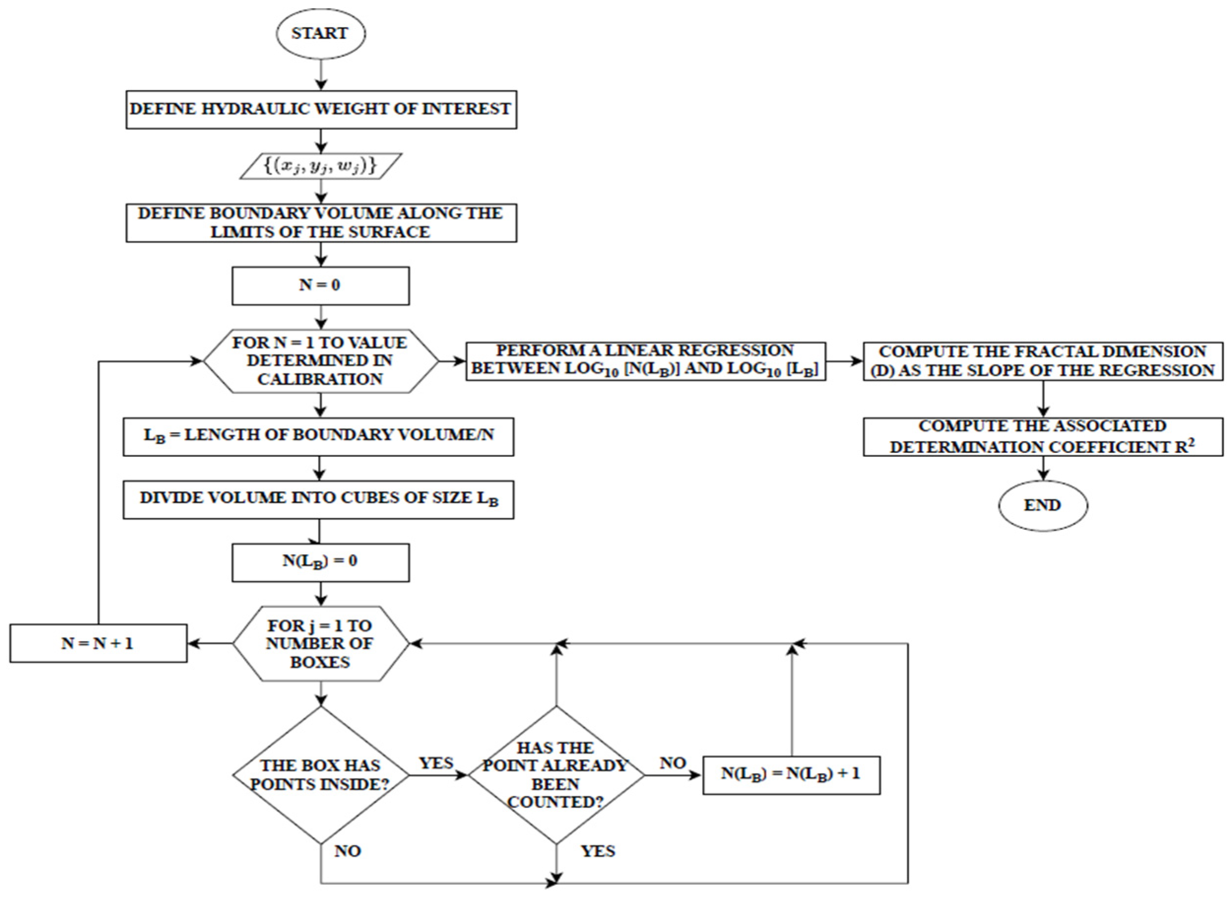
2.2. Fractal Analysis

Song et al. [42,43,44] demonstrated that the algorithm for computing D [as in Equation (1)] is equivalent to vertex coloring in arbitrary networks, leading to the development of the widely used box-covering algorithm. Wen et al. [54] compared multiple algorithms for fractal analysis—including box-covering (standard and weighted), burning, and sandbox methods—and found that while all yielded similar D values in urban networks (including WDS [27]), the box-covering algorithm was the most commonly applied. Kim et al. [55] later proposed a computationally efficient alternative based on a random branching tree with local shortcuts, noting that it produced comparable results to Song’s method but with improved performance.
Given the established link between D and network topology, this study first assessed the suitability of the selected case studies for fractal analysis. Goh et al. [56] and Kim et al. [55] showed that tree-like structures can represent real-world fractals, making D values comparable across different geometric and connectivity patterns. Csányi et al. [57] further confirmed that both small and large networks exhibit similar fractal behavior, with larger networks typically showing higher D values but still satisfying the same power law.
Based on these findings, this study applies the box-covering algorithm across a range of case studies of varying sizes and topological configurations, ensuring the comparability and reliability of the performed fractal analysis.
The fractal analysis starts by computing the fractal dimension of the OHGS. This research employs the fractal dimension of the OHGS computed by Jaramillo et al. [36], given that constructing the OHGS requires several procedures to characterize the properties of this smooth surface. Further details on the construction of the OHGS can be found in Jaramillo [58] and Jaramillo et al. [36,37]. When the OHGS is obtained, its fractal dimension is calculated using an adapted variation estimation method based on the work of Tolle et al. [59] and Zhou et al. [60]. This decision was made given that there is no further research analyzing the fractal dimension of the OHGS, and since this research focuses on the box-covering magnitudes of D, these values serve as a reference that allows a direct comparison between previous research and this study.

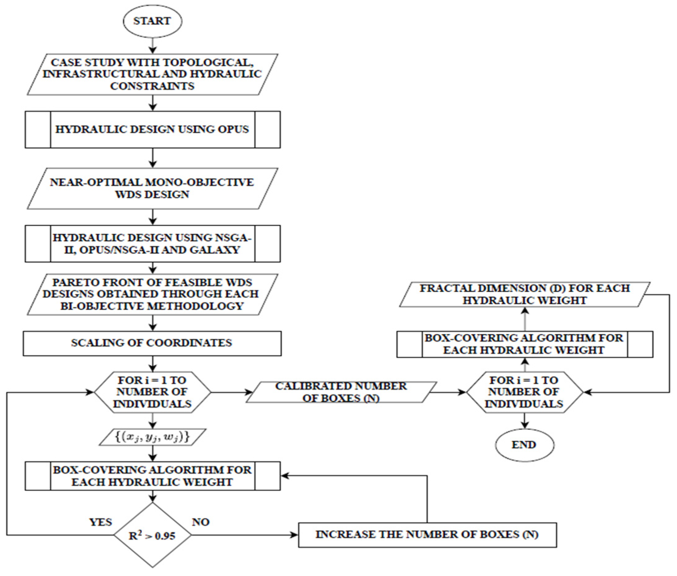
2.3. Fractal Analysis of the Design Outcomes

The computation of D requires the steady state hydraulic modelling to estimate flow variables that characterize the fractal analysis criteria (wj). As explained before, the fractal understanding of WDS refers to the study of the real energy distribution pattern of the real HGS with respect to the ideal energy distribution pattern of the OHGS of near-optimal solutions.
In the box-covering algorithm, the HGS is understood as the set of geometrical coordinates (xj, yj, HGLj) that build a surface by interpolation. In addition, the distribution of diameters (d) conforming surfaces of coordinates (xj, yj, Σdij) and the distribution of flow rates conforming surfaces of coordinates (xj, yj, ΣQij) at the nodes of WDS are obtained. The additional surfaces constructed considering diameters and flow rate distributions are usually obtained while performing fractal analysis to determine possible correlations between energy distribution, diameter, and flow rate distributions. In this sense, this research considered three (3) hydraulically based fractal analysis criteria (wj) [see Equations (2)–(4)]. Equation (2) represents the energy (HGL) criterion, which refers to the piezometric head (HGL) values at the j-th demand node. Equation (3) represents the infrastructural (d) criterion, which calculates the sum of the diameter values of the i pipes connected to the j-th node. Equation (4) is used to compute the flow criterion (Q), which calculates the sum of the flow rate (Q) of the i pipes connected to the j-th node.
w j = H G L j
w j = i d i j
w j = i Q i j
After storing the {(xj, yj, wj)} surface for a given criterion and WDS of analysis, the box-covering algorithm defines a boundary volume; in this case, a cube that encompasses all the points. Then, this volume is partitioned into equally sized boxes with a side length LB, where LB is decreased incrementally from a larger value to a smaller value. The algorithm iterates through all the boxes, checking if there are points within each box. Duplicated points that have been counted in more than one box are then eliminated. Finally, the number of boxes required to cover the entire WDS is recorded and the algorithm proceeds to the next iteration using a smaller box size (LB).
By counting the number of boxes with points inside them, the box-covering algorithm estimates the minimum number of boxes required to cover the nodes of a WDS. The box-covering approach considers a WDS as a fractal body if the number of covering units N(ε) and their box length (LB) follow a power law relationship [see Equation (5)]. Compared with Equation (1), the number of covering units N(ε) corresponds to the measured quantity across the fractal, while the box length (LB) represents the scale of analysis [see Equation (1)].
N L B ~ L B D
By applying the logarithm to both sides of Equation (5), it is possible to compute the fractal dimension (D) using a linear regression with determination coefficient R2. Consequently, the fractal dimension (D) is determined as the slope of the resulting linear regression. Figure 1 shows the steps of the box-covering algorithm performed in this study.
The fractal dimension of the box-covering algorithm falls within the range D ∈ [1, OHGS), where OHGS represents the fractal dimension of the Optimal Hydraulic Gradient Surface. The lower boundary is D = 1, given that this would be the fractal dimension (D) of a line. On the other hand, the upper boundary corresponds to the fractal dimension of the OHGS given the hypothesis that D can exceed the value expected for a flat surface (D = 2) but is restricted by the ideal fractal dimension of the OHGS. Theoretically, feasible WDS designs do not reach the OHGS due to pressure, velocity and topological constraints.
As stated before, to ensure robust D magnitudes, the number of boxes with side length (LB) was calibrated to maximize the determination coefficient R2. The objective was to obtain significant D magnitudes across all analyzed hydraulic designs from the bi-objective approach. According to Diao et al. [25], statistically significant D magnitudes are obtained when their associated determination coefficients R2 > 0.95. Hence, in this study, the number of boxes of length size (LB) was increased until determination coefficients R2 > 0.95 were achieved for the fractal dimensions (D) of all fractal analysis criteria (wj). Additionally, the {(xj, yj, wj)} points were scaled to ensure a consistent relationship between the orders of magnitude of the horizontal coordinates and their corresponding weights (wj). In this research, the scaling was performed as proposed by Saldarriaga et al. [38]; i.e., the weight (wj) magnitudes were defined to be of a 10−2 order of magnitude smaller than the scaled horizontal coordinates, which were set to a 103 order of magnitude. This approach facilitated obtaining comparable fractal dimension (D) magnitudes among the analyzed WDS.
Figure 2 shows the complete methodology of this research. As explained before, hydraulic designs were initially obtained following mono-objective and bi-objective approaches. Then, each case study followed a calibration process to ensure fractal dimensions (D) with R2 > 0.95 among all design individuals and methodologies. Later, geometrical scaling was performed to obtain comparable fractal dimensions (D) among case studies. Finally, fractal dimensions (D) for each hydraulic weight (wj) were computed.

2.4. Sensitivity Analysis

Previous research has explored different applications of fractal analysis in the operation processes of WDS. This research was conducted to analyze the implications of D in operation through a sensitivity analysis. Previous studies focused on particular applications, but the main gap in the field of operation refers to the variation in D when operational conditions deviate significantly from design conditions. In this sense, the sensitivity of D to operational extremes was studied considering pipe roughness increase due to pipe aging and nodal demand increase due to population growth.
First, near-optimal OPUS designs were obtained using the design parameters and the appropriate hydraulic equations for each case study found in the literature [6]. Then, pipe roughness magnitudes and nodal demands (Qd) were varied. Later, the corresponding hydraulic criteria (wj) defined in Equations (2)–(4) were recorded. Finally, from the stored weights (wj), D magnitudes were computed.
To understand the response of D to pipe roughness magnitudes, near-optimal OPUS designs were computed varying the roughness coefficients of the considered case studies using the roughness multipliers MPi inside the set MP [see Equation (6)].
M P = M P i | M P i Z + , 1 M P i 10
In addition, to understand the response of D to nodal demands (Qd), near-optimal OPUS designs were computed varying the base demand (Qd) values of the considered WDS using the demand multipliers MPi inside the set MP [see Equation (6)]. In the sensitivity analysis, the multipliers MPi were chosen to induce a significant increase in the analyzed property—roughness or demands—within the WDS that allowed to observe clear sensitivity in the behavior of the computed D values.

3. Case Studies

Four benchmark WDS were considered in this study to test the proposed analysis: Hanoi [45], Balerma [46], Pescara, and Modena [47] (see Figure 3). Table 1 presents the main characteristics of each network, including cost parameters, design constraints, and the size of the problem. The latter table also shows the fractal dimension of the Optimal Hydraulic Gradient Surface, obtained from previous studies [36]. Fractal dimension magnitudes of the OHGS are comparable between networks of different sizes and topological patterns (see OHGS in Table 1) according to the tree-like structure interpretation and the scale invariance of real-life fractals [55,56,57]. Hence, results will remain comparable across case studies despite the varying topological configurations.
Table 2 shows the design parameters used to perform fractal analysis in this study, considering the algorithms described in the methodology. A detailed explanation of each design parameter can be found in the Supplementary Materials.

4. Results

This section presents the optimal designs obtained following the mono and bi-objective approaches using the various optimization methods described above. Then, the fractal dimension (D) results of the mono-objective and bi-objective approaches are presented for each case study. Later, a sensitivity analysis shows the response of D to the variations in pipe roughness and nodal demands.

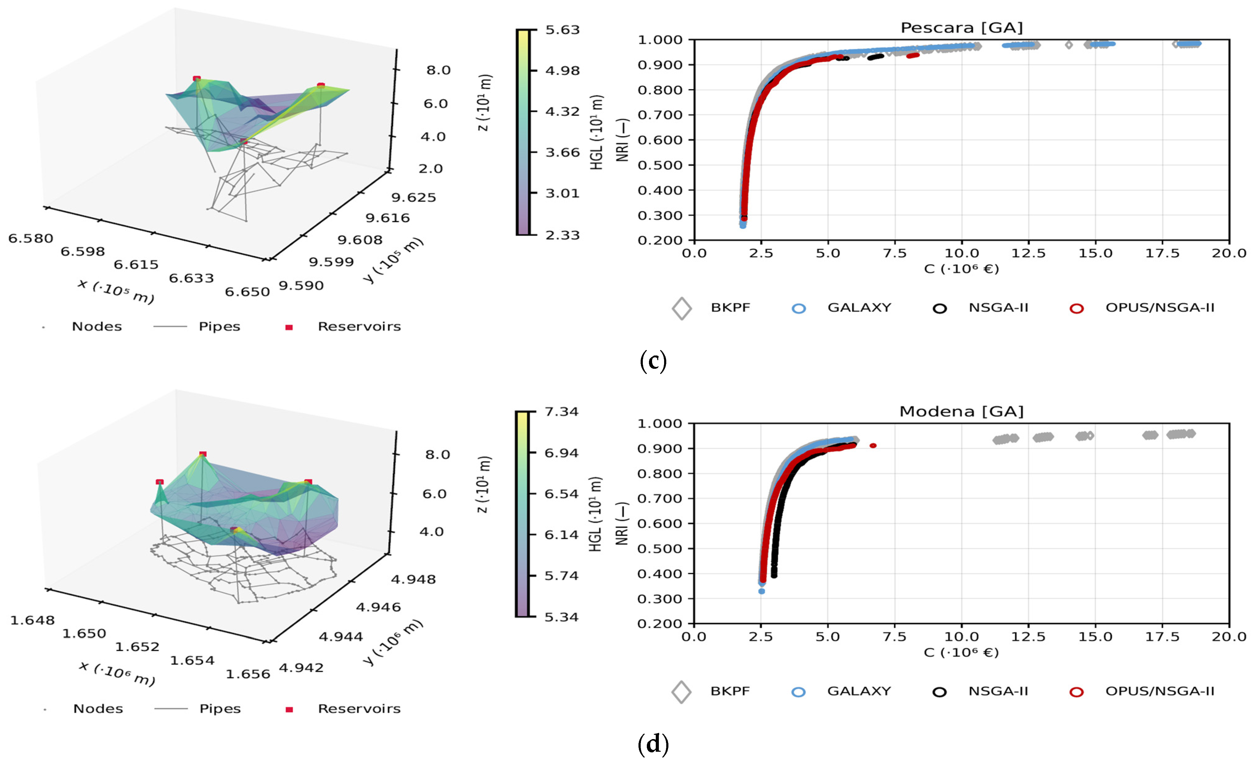
4.1. Optimal Designs

Figure 4 shows the results of the optimal designs of the mono-objective and bi-objective approaches for the tested case studies. The left panel shows the interpolated HGS obtained using OPUS in the mono-objective algorithm. The right panel shows the comparison between the Pareto Fronts (PF) obtained using the biobjective optimization methods with the best-known PF [2]. Details on the mono-objective design outcomes can be found in Section S3.1 of the Supplementary Materials, while the bi-objective designs are available in Section S3.2. The solutions of Figure 4 approximate the best-known PF found in the literature and capture a wide range of cost (C)–NRI combinations to perform fractal analysis.

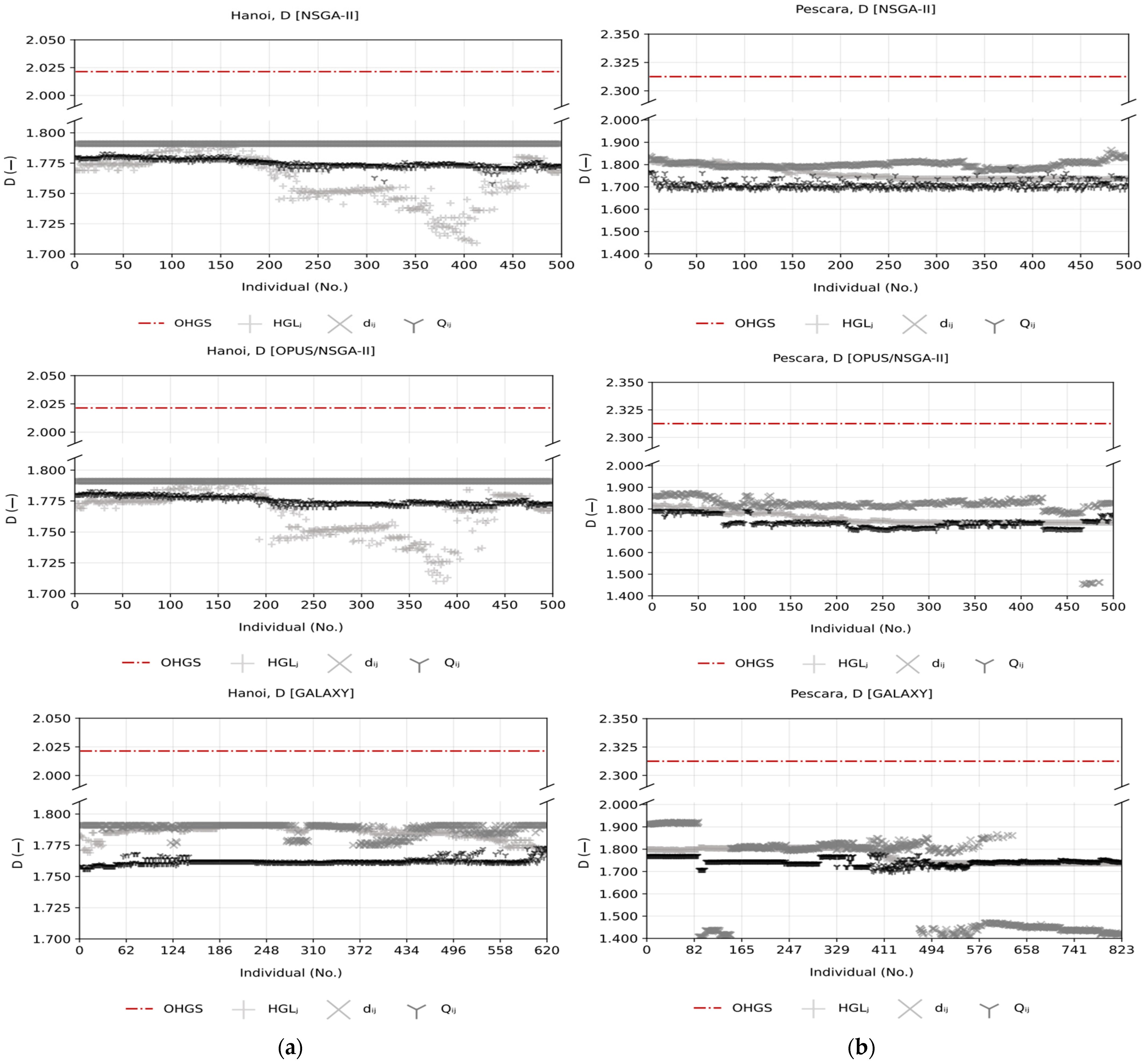
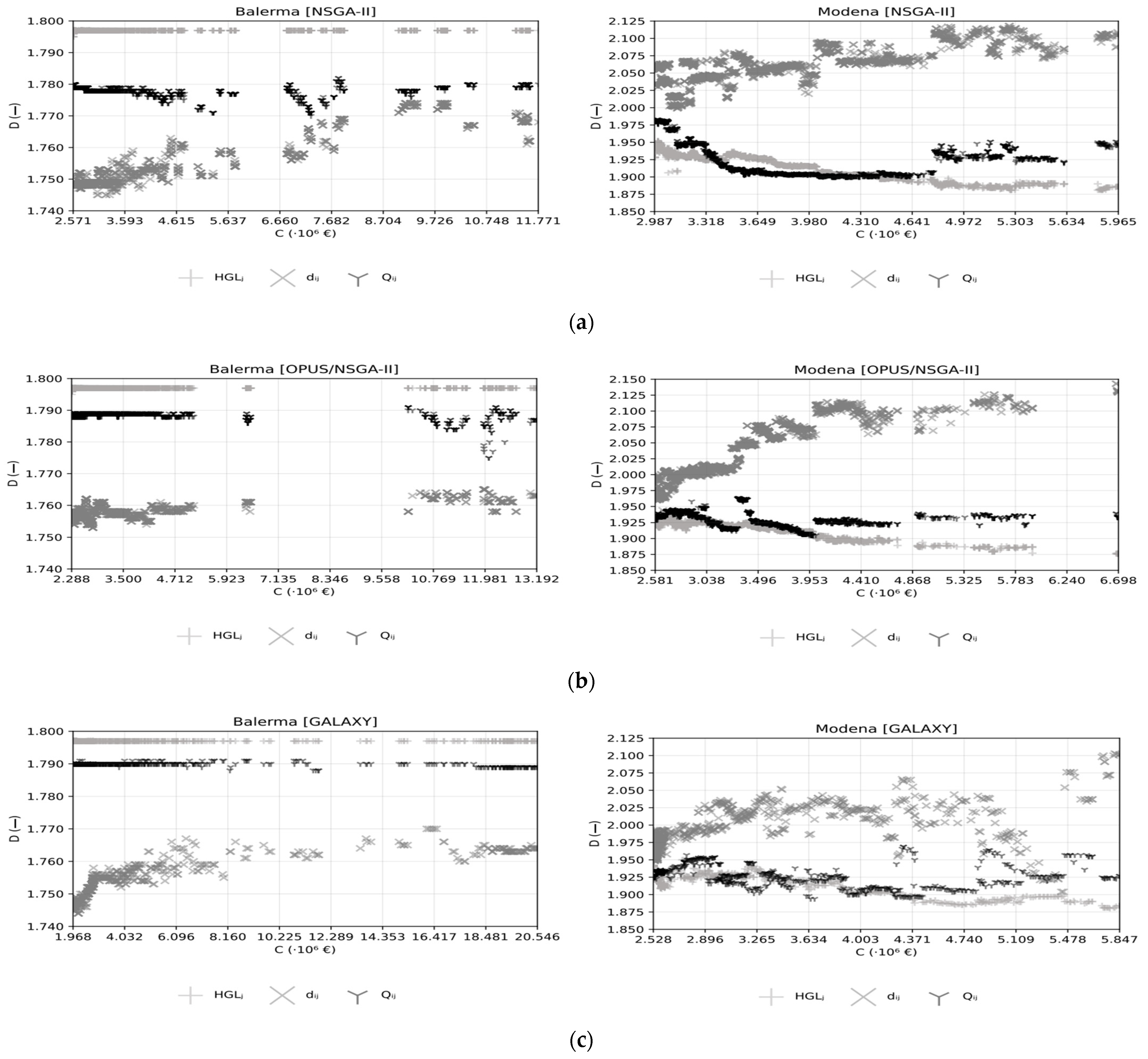
4.2. Fractal Analysis

Using the optimal designs shown above, D magnitudes were obtained, ultimately determining whether the resulting designs were fractal or not based on R2. Table 3 and Table 4 present the results of the box-covering algorithm for the mono-objective and bi-objective optimization approaches, including the achieved D magnitudes, and the associated determination coefficient (R2) of each criterion by case study. Given that the box-covering algorithm was able to compute D of high significance (R2 > 0.95) among all case studies, this confirms that WDS are self-similar fractals. Hence, WDS exhibit repeating patterns at different scales, maintaining consistent geometric similarity regardless of the level of magnification.
For the mono-objective approach, Table 3 includes the corresponding percent errors (%E) with respect to the fractal dimension of the OHGS obtained by Jaramillo [36] inside parentheses. These results suggest that the differences between the D magnitudes and the fractal dimension of the OHGS are consistent across case studies and vary within similar ranges, as %EHGLⱼ ∈ [11.547%, 21.427%], %Edᵢⱼ ∈ [11.007%, 23.941%] and %EQᵢⱼ ∈ [12.486%, 23.763%].
With respect to the bi-objective approach, the high significance (R2 > 0.95) remained throughout all iterations by methodology (see Section S3.2 of the Supplementary Materials), which suggests that fractality does not depend on the cost (C) or hydraulic behavior of each individual (consequence of the design) but on the topology of the network. For instance, Hanoi—the simplest topology with the lowest D—was not very responsive to changes in the fractal criteria, whereas Modena—the most complex topology with a higher D—exhibited variation across the different tested criteria.
The latter observation was assessed by analyzing the variation in D magnitudes across individuals (in bi-objective approaches). Thus, Figure 5 displays the results for Hanoi (strong fractal) and Pescara (weak fractal) after sorting the associated costs (C) in ascending order. In Figure 5, the behavior of Pescara exhibited significant variation among individuals with different costs, particularly for wj = Σidij. However, this relationship is not controlled by the design cost (C) or the hydraulic properties but rather by the weak fractal behavior of the network, given that its associated determination coefficients could be as low as R2 = 0.952. In contrast, the behavior of Hanoi shows that, regardless of cost (C), D remains nearly constant, meaning that D does not depend on the cost (C) or the hydraulic properties of the design outcome. Similarly, the presented results from Table 3, Table 4, and Figure 5 indicate that D does not approach the fractal dimension of the OHGS in minimum cost designs. Detailed results for each case study and optimization method are shown in Section S3.3 of the Supplementary Materials.

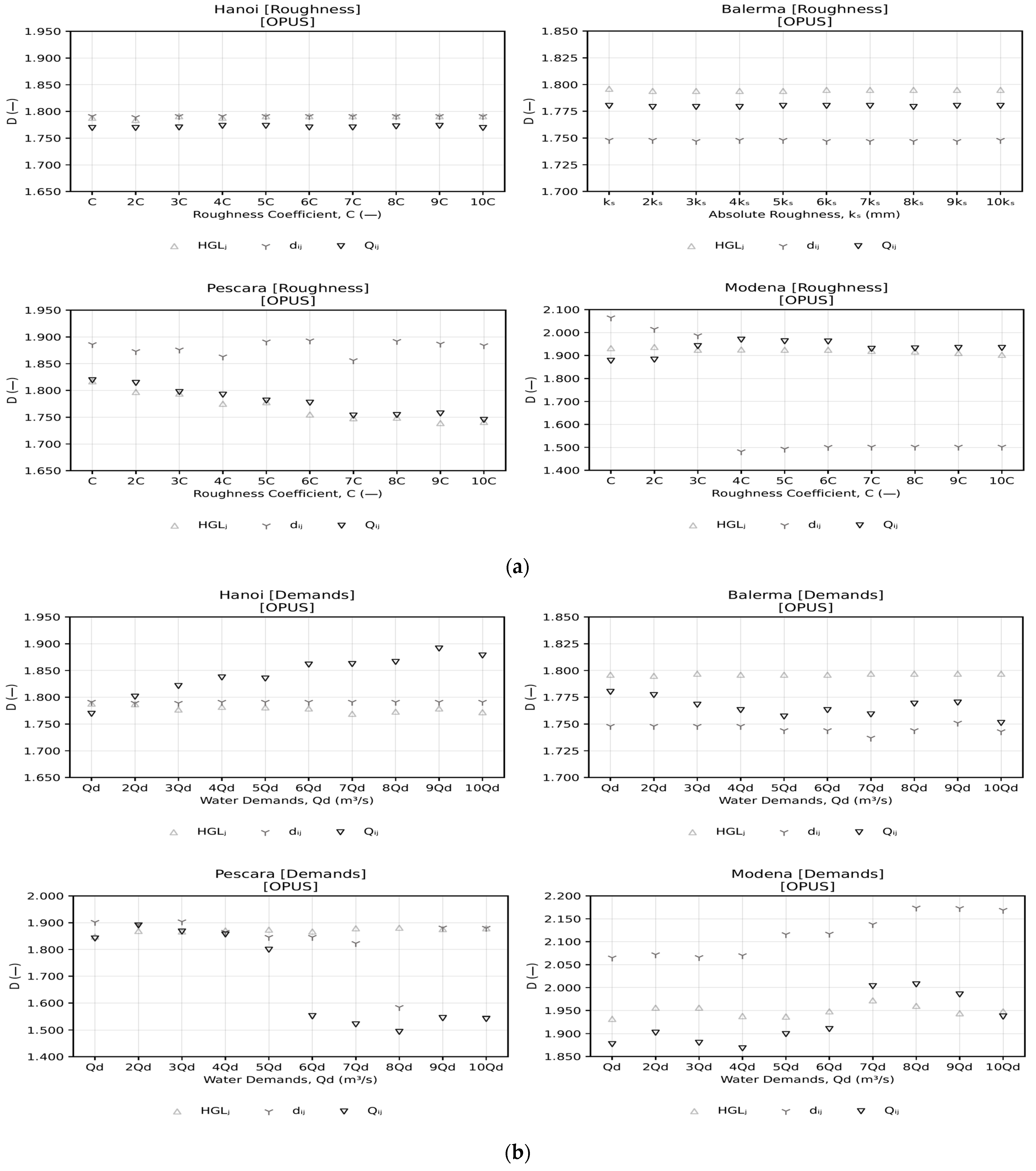
4.3. Sensitivity Analysis

Figure 6a illustrates the pipe roughness sensitivity analysis results. In Figure 6a, D was nearly constant and did not vary significantly along the range D ∈ [1, OHGS) for any of the case studies. However, note that in some cases of Figure 6a, such as Pescara and Modena, D tends to become smaller and weaker (R2 > 0.95) when pipe roughness magnitudes increase. Even if there is a near-constant tendency in some of the case studies, the weak fractal behavior of Pescara and Modena can be further studied. This is because there can be a link between increased pipe roughness and weak fractal behavior. In the operation of WDS, weak D in a self-similar portion of calibrated pipes of a WDS could indicate aging or increased rugosities of a larger portion of pipes of the system, such as the pipes in a hydraulic sector. This is a future avenue of research that needs to be investigated.
Figure 6b shows the results of the water demand (Qd) sensitivity analysis. In Figure 6b, the magnitudes of D were nearly constant and did not vary significantly along D ∈ [1, OHGS) for any case study. However, the observed weak fractal behavior of Pescara [see Figure 6b] can be useful in the operation of WDS, as weak D in a self-similar portion of calibrated pipes within the system could serve as indicators of variations in nodal demands (Qd) in larger portions of the system due to population increase.
The association between weak fractal behavior and the increase in pipe roughness or in nodal demands (Qd) cannot be completely explained by these results, as the weak fractal behavior may be influenced by other factors such as the headloss equation used in the analysis. However, this operational avenue that uses D should be analyzed in further studies since it has not been sufficiently explored in previous works.

4.4. Computational Requirements

Over a period of five (5) months, nine (9) computer devices were employed to conduct this research. The hydraulic modeling was performed using EPANET [61], while the mono-objective designs were obtained through REDES [50]. For the implementation of GA, the EPANET-MATLAB Toolkit [62] was employed, and the computation of D involved the use of WNTR [63]. The devices had diverse processors ranging between Intel Core™ i5-i9, Intel Xeon®, and AMD Ryzen™ 5, clock speeds between 1.40 GHz to 3.20 GHz using 1 or 2 cores, and RAM storage capacities ranging from 4 GB to 256 GB.
The computational time required by each iteration depended on the ability of the box-covering algorithm to identify fractal behavior in the studied individuals. In individuals that did not exhibit weak fractal behavior, the computational time depended on the general complexity of the WDS. This meant 5 to 10 min by iteration in Hanoi and 15 to 20 min by iteration in Balerma. On the other hand, weaker fractals, such as Pescara and Modena, employed much larger computational time, as the algorithm was required to transit further in space to identify the fractal correlation of the studied individuals. This meant 55 to 60 min by iteration in Pescara and 25 to 30 min by iteration in Modena.

5. Analysis of Results

5.1. Fractal Behavior in WDS

WDS are self-similar fractal bodies. The mono-objective and bi-objective optimal designs consistently demonstrated similar D outcomes across all analyzed criteria (wj). Indeed, the computed D magnitudes for each criterion showed high repeatability, i.e., D magnitudes were similar to each other and exhibited small deviation with respect to the fractal dimension of the OHGS. Moreover, D always ranged along D ∈ [1, OHGS) with robust determination coefficients R2 > 0.95 (see Table 3 and Table 4). These findings confirm that WDS are self-similar fractal bodies.
The importance of WDS being self-similar fractal bodies implies the exhibition of repeating patterns at different scales in the topology that maintain consistent geometric similarity regardless of the level of magnification. In practical terms, this implies that an isolated set of pipes in the network, for example, the set of pipes of a DMA, has the same fractal behavior as the whole network. The latter suggests the possibility of using D to understand the behavior of a complete WDS by analyzing its parts, a computational advantage when dealing with large-scale networks.

5.2. D as an Indicator of Optimality

Table 3 and Table 4 show that D magnitudes obtained from mono-objective and bi-objective optimal designs considering all fractal analysis criteria (wj) differ from the fractal dimension of the OHGS and never reach this value. These results confirm the findings of previous research, i.e., that optimized WDS designs seek to mimic the ideal energy distribution of the OHGS, but the constraints of the problem (topological, design, and hydraulic) impose a final HGS that deviates from the ideal energy distribution and fractal behavior.
To further explore D as an indicator of optimality, Figure 7 shows the comparison between D and the cost (C) of Balerma (strong fractal) and Modena (weak fractal). In both cases, there was not a clear correlation between D and cost (C) among design methodologies or fractal analysis criteria (wj), meaning that D is not dependent on the design cost (C) of the WDS. Therefore, D cannot serve as an indicator of optimality by itself. Moreover, as the metrics of resilience are inversely correlated with respect to the cost (C) of a WDS in a PF, D is not correlated with resilience measured through NRI. These results establish that, when the algorithm is calibrated for each WDS, geometrical coordinates are scaled equally between case studies and a wider range of individuals are analyzed, D does not depend on the properties of the design outcomes. Once again, results suggest that D only depends on the topological configuration of each case study. Additional figures showing the comparison for Hanoi and Pescara can be found in Section S3.2 of the Supplementary Materials.

5.3. Significance of the Topology in D

As observed before, D only depends on the topology. However, the resulting magnitudes of fractal dimension (D) exhibited low sensitivity to the constructive cost (C), energy (HGL), infrastructural (d), and flow (Q) distributions between individuals. The latter result was expected given that D is self-compared within a specific WDS. The self-compared nature is understood in terms of non-Euclidean geometrical complexity. For example, from a mathematical standpoint, if the distribution of diameters (d) within an individual exhibits significant discrepancy across different regions of a WDS, the overall geometrical structure becomes more irregular, resulting in augmented complexity that achieves higher D values. This marginal sensitivity of D is observed in Figure 5 and Figure 7.
Given the topological description of D, this research proposes final D magnitudes for each case study for further research of fractality in WDS (see Table 5). The final D magnitudes of Table 5 were computed as the mean of all the values obtained through the mono-objective and bi-objective approaches, as well as the pipe roughness and demand sensibility analysis, segregating values by fractal analysis criterion (wj). The final D value in the last column of Table 5 corresponds to the mean of all the values by case study reported in this paper.
Table 6 presents the D magnitudes previously reported by Jaramillo et al. [36] and compares these values with the computed values from Table 5. The differences between D magnitudes reported in the existing literature and those obtained in this study are substantial and can be attributed to multiple factors. First, the calibration process used in this study ensured that all design individuals had fractal dimensions with R2 > 0.95, which accounts for the discrepancies observed in the previously reported D magnitudes, particularly for Hanoi and Modena. Second, this study applied geometrical coordinate scaling to achieve comparable magnitudes between (xj, yj) coordinates and hydraulic criteria (wj). The latter step was not performed in previous research, leading to significant discrepancies in the reported results across all case studies.
Additionally, some of the results reported by Jaramillo et al. [45] present mathematical inconsistencies, as D values lower than 1 (D < 1) are not possible in WDS due to their geometric approximation to a surface that would theoretically approach to D = 2. However, Table 6 shows that D < 1 for Balerma and Pescara, which contradicts the HGS construction approach, where the hydraulic gradient line (HGL) values were interpolated across a geometric surface. This discrepancy suggests a misinterpretation of the fractal properties of these networks in previous analyses.
The values of Table 6 approximated the fractal understanding of WDS. This means that they presented a framework for analyzing WDS based on CNT. However, in this previous work, the underlying complexity of the fractal description of WDS was not fully understood through the lens of GT, and this led to the exclusion of topology from the analysis.
The results in this study showed that D depends on the topology, resolving previous issues that existed between the preliminary conclusions relating cost (C), D, and resilience (NRI). These findings suggest that D should not be used to establish relationships between classic design metrics, such as cost (C) or resilience (NRI), but that D should be used to investigate topology by itself.

6. Conclusions and Future Work

This paper assessed the box-covering fractal dimension (D) as a design and operation criterion by inspecting the relationship between topology, cost (C), and resilience (NRI) in water distribution systems (WDS). To achieve this goal, fractal dimensions (D), following the energy (wj = HGLj), infrastructural (wj = Σdij), and flow (wj = ΣQij) criteria were computed using a box-covering algorithm calibrated and scaled based on graph theory (GT) considerations. The algorithm was performed in four (4) case studies: Hanoi, Balerma, Pescara, and Modena. Design individuals were obtained following a mono-objective that used OPUS and a bi-objective approach that used feasible design individuals obtained through NSGA-II, OPUS/NSGA-II, and GALAXY. The key takeaways from the presented results are summarized as follows:
  • WDS are self-similar fractal bodies.
  • Fractal dimension (D) magnitudes are restricted by the underlying complexity of WDS.
  • The fractal dimension (D) does not approach the fractal dimension of the OHGS in minimum cost designs.
  • The fractal dimension (D) does not depend on the design cost (C) of the WDS.
  • The fractal dimension (D) only depends on the topology.
Furthermore, the results indicated that the fractal dimension (D) does not serve as an optimality indicator but as a tool for analyzing and constructing the topology of WDS. In this regard, the topology dependence opens a new avenue of research related to WDS design. This research identified several long-term strategies to investigate the topological avenue of WDS design that are based on the mathematical interpretation of D derived from fractal analysis. Long-term strategies that can be investigated are the following:
  • Fractal-based topologies inspired by natural drainage patterns can be used to redesign WDS. The fractal topologies can be used to subsequently perform the diameter (d) selection process using algorithms like NSGA-II to evaluate if fractal topologies improve the resulting cost (C) and resilience (NRI) of the design outcomes.
  • D can guide the iterative definition of WDS layouts, aiming to replicate the structural properties of reference systems.
  • D can function as an indicator of redundancy, with higher values reflecting increased pipe interconnections; this can support compliance with regulatory redundancy standards.
  • Fractal analysis might be extended to operational aspects of WDS, helping to understand effects related to pipe roughness and nodal demand (Qd) increase.
All the presented avenues for future research are supported by the presented GT literature of fractal analysis applied in the context of urban networks. In addition, these approaches are not computationally expensive, as a few iterations would be required to achieve the desired D magnitude, given its nearly constant nature and the computational advantage of self-similarity.
In the short term, the results presented in this research only refer to the conclusion of the topological dependence of D and to the obtention of robust D magnitudes that can serve to investigate the proposed long-term strategies. In this regard, the presented results have a set of limitations that need to be addressed when investigating the proposed long-term approaches. First, the presented results are applicable to the presented case studies, and this means that other case studies need to follow a similar procedure before being able to derive the design and operation frameworks that can be generalized among all WDS. In addition, the proposed approaches are still preliminary, given that there is still no understanding of appropriate mechanisms of topological iteration that simultaneously derive hydraulically viable WDS, i.e., topological configurations that use the initial energy input at water sources and satisfy the continuity equation, the conservation of mass at the demand nodes (NND), and the hydraulic design constraints. This means that the topological iteration framework based on D needs particular attention in future research. Third, even if D was compared with cost (C) and resilience (NRI) to derive the topological dependency conclusion, additional network metrics need to be assessed to investigate whether the marginal sensitivity spotted in D outputs among design individuals is correlated with sensitivity in these indexes. The correlation between D, the Branch Index (BI), and the Meshedness Coefficient (MCO-R) was preliminarily studied by Saldarriaga et al. [38] by investigating the classification system of WDS proposed by Hwang and Lansey [8], which is based on these indexes. The preliminary results of this research indicated no correlation between D sensitivity and change in WDS classification of the design individuals. However, this analysis must be performed in future studies to derive a fractal-based design framework based on topological iteration.
Future research needs to continue investigating the proposed approaches by identifying techniques generalizable to WDS with different topological, energy (HGL), infrastructural (d), and flow (Q) distribution patterns, and by studying the behavior of the fractal dimension (D) in real-life WDS. The robust fractal dimensions (D) derived from this research are pivotal outcomes, serving as essential references for rigorously testing and validating the proposed approaches. The present results are promising, and fractal analysis may be the key tool for achieving a mathematical description of the hydraulic design and operation of WDS.

Supplementary Materials

The following supporting information can be downloaded at: https://www.mdpi.com/article/10.3390/w17091318/s1, Complete NSGA-II, OPUS/NSGA-II, GALAXY design outputs; Detailed box-covering D outputs.

Author Contributions

Conceptualization, S.G. and J.S.; methodology, S.G., C.S. and J.S.; software, S.G.; validation, C.S., L.G. and J.S.; formal analysis, S.G., C.S. and J.S.; investigation, S.G., L.G. and J.S.; resources, S.G. and J.S.; data curation, S.G.; writing—original draft preparation, S.G. and L.G.; writing—review and editing, S.G., C.S. and J.S.; visualization, S.G.; supervision, C.S. and J.S.; project administration, S.G. and J.S. All authors have read and agreed to the published version of the manuscript.

Funding

This research received no external funding.

Data Availability Statement

The original contributions presented in this study are included in the article/Supplementary Materials. Further inquiries can be directed to the corresponding author.

Acknowledgments

To Wang Q., for providing the design outputs of GALAXY.

Conflicts of Interest

The authors declare no conflicts of interest.

References

  1. EPA. Drinking Water Infrastructure Needs Survey and Assessment; EPA: Washington, DC, USA, 2025.
  2. Wang, Q.; Guidolin, M.; Savic, D.; Kapelan, Z. Two-Objective Design of Benchmark Problems of a Water Distribution System via MOEAs: Towards the Best-Known Approximation of the True Pareto Front. J. Water Resour. Plan. Manag. 2015, 141, 04014060. [Google Scholar] [CrossRef]
  3. Yates, D.F.; Templeman, A.B.; Boffey, T.B. The Computational Complexity of the Problem of Determining Least Capital Cost Designs for Water Supply Networks. Eng. Optim. 1984, 7, 143–155. [Google Scholar] [CrossRef]
  4. Cunha, M.d.C.; Sousa, J. Water Distribution Network Design Optimization: Simulated Annealing Approach. J. Water Resour. Plan. Manag. 1999, 125, 215–221. [Google Scholar] [CrossRef]
  5. Geem, Z.W.; Kim, J.H.; Loganathan, G.V. A New Heuristic Optimization Algorithm: Harmony Search. Simulation 2001, 76, 60–68. [Google Scholar] [CrossRef]
  6. Saldarriaga, J.; Páez, D.; Salcedo, C.; Cuero, P.; López, L.L.; León, N.; Celeita, D. A Direct Approach for the Near-Optimal Design of Water Distribution Networks Based on Power Use. Water 2020, 12, 1037. [Google Scholar] [CrossRef]
  7. Sitzenfrei, R.; Wang, Q.; Kapelan, Z.; Savić, D. Using Complex Network Analysis for Optimization of Water Distribution Networks. Water Resour. Res. 2020, 56, e2020WR027929. [Google Scholar] [CrossRef]
  8. Hwang, H.; Lansey, K. Water Distribution System Classification Using System Characteristics and Graph-Theory Metrics. J. Water Resour. Plan. Manag. 2017, 143, 04017071. [Google Scholar] [CrossRef]
  9. Carvajal, J.; Ariza, A.; Saldarriaga, J. Advanced Geometrical Analysis of Water Distribution Networks (WDNs): A Comparison between Standard and Minimum Capital-Cost Designs. In Proceedings of the World Environmental and Water Resources Congress 2021, Virtual, 7–11 June 2021; American Society of Civil Engineers: Reston, VA, USA, 2021; pp. 914–924. [Google Scholar]
  10. Rana, S.M.M.; Boccelli, D.L.; Marchi, A.; Dandy, G.C. Drinking Water Distribution System Network Clustering Using Self-Organizing Map for Real-Time Demand Estimation. J. Water Resour. Plan. Manag. 2020, 146, 04020090. [Google Scholar] [CrossRef]
  11. Abokifa, A.A.; Sela, L. Identification of Spatial Patterns in Water Distribution Pipe Failure Data Using Spatial Autocorrelation Analysis. J. Water Resour. Plan. Manag. 2019, 145, 04019057. [Google Scholar] [CrossRef]
  12. Perelman, L.; Ostfeld, A. Topological Clustering for Water Distribution Systems Analysis. Environ. Model. Softw. 2011, 26, 969–972. [Google Scholar] [CrossRef]
  13. Qiu, M.; Ostfeld, A. Dynamic Clustering for Water Distribution System Water Quality Management. In Proceedings of the World Environmental and Water Resources Congress 2020, Henderson, NV, USA, 17–21 May 2020; American Society of Civil Engineers: Reston, VA, USA, 2020; pp. 318–328. [Google Scholar]
  14. Alvisi, S.; Franchini, M. Calibration and Sensitivity Analysis of the C-Town Pipe Network Model. In Proceedings of the Water Distribution Systems Analysis 2010, Tucson, AZ, USA, 12–15 September 2010; American Society of Civil Engineers: Reston, VA, USA, 2011; pp. 1573–1584. [Google Scholar]
  15. Diao, K.; Zhou, Y.; Li, J.; Liu, Z. Battle of the Water Calibration Networks (BWCN): A Component Status Changes Oriented Calibration Method for Zonal Management Water Distribution Networks. In Proceedings of the Water Distribution Systems Analysis 2010, Tucson, AZ, USA, 12–15 September 2010; American Society of Civil Engineers: Reston, VA, USA, 2011; pp. 1629–1644. [Google Scholar]
  16. Scibetta, M.; Boano, F.; Revelli, R.; Ridolfi, L. Community Detection as a Tool for District Metered Areas Identification. Procedia Eng. 2014, 70, 1518–1523. [Google Scholar] [CrossRef]
  17. Ferrari, G.; Savic, D.; Becciu, G. Graph-Theoretic Approach and Sound Engineering Principles for Design of District Metered Areas. J. Water Resour. Plan. Manag. 2014, 140, 04014036. [Google Scholar] [CrossRef]
  18. Buhl, C.; Gautrais, J.; Reeves, N.; Solé, R.V.; Valverde, S.; Kuntz, P.; Theraulaz, G. Topological Patterns in Street Networks of Self-Organized Urban Settlements. Eur. Phys. J. B-Condens. Matter Complex Syst. 2006, 49, 513–522. [Google Scholar] [CrossRef]
  19. Lämmer, S.; Gehlsen, B.; Helbing, D. Scaling Laws in the Spatial Structure of Urban Road Networks. Phys. A Stat. Mech. Its Appl. 2006, 363, 89–95. [Google Scholar] [CrossRef]
  20. Barthélemy, M.; Flammini, A. Co-Evolution of Density and Topology in a Simple Model of City Formation. Netw. Spat. Econ. 2009, 9, 401–425. [Google Scholar] [CrossRef]
  21. Yang, S.; Paik, K.; McGrath, G.S.; Urich, C.; Krueger, E.; Kumar, P.; Rao, P.S.C. Functional Topology of Evolving Urban Drainage Networks. Water Resour. Res. 2017, 53, 8966–8979. [Google Scholar] [CrossRef]
  22. Krueger, E.; Klinkhamer, C.; Urich, C.; Zhan, X.; Rao, P.S.C. Generic Patterns in the Evolution of Urban Water Networks: Evidence from a Large Asian City. Phys. Rev. E 2017, 95, 032312. [Google Scholar] [CrossRef]
  23. Zischg, J.; Reyes-Silva, J.D.; Klinkhamer, C.; Krueger, E.; Krebs, P.; Rao, P.S.C.; Sitzenfrei, R. Complex Network Analysis of Water Distribution Systems in Their Dual Representation Using Isolation Valve Information. In Proceedings of the World Environmental and Water Resources Congress 2019, Pittsburgh, PA, USA, 19–23 May 2019; American Society of Civil Engineers: Reston, VA, USA, 2019; pp. 484–497. [Google Scholar]
  24. Falconer, K. Fractal Geometry; Wiley: Hoboken, NJ, USA, 2003; ISBN 9780470848616. [Google Scholar]
  25. Diao, K.; Butler, D.; Ulanicki, B. Fractality in Water Distribution Networks: Application to Criticality Analysis and Optimal Rehabilitation. Urban. Water J. 2021, 18, 885–895. [Google Scholar] [CrossRef]
  26. Pentland, A.P. Fractal-Based Description of Natural Scenes. IEEE Trans. Pattern Anal. Mach. Intell. 1984, PAMI-6, 661–674. [Google Scholar] [CrossRef]
  27. Kowalski, D.; Kowalska, B.; Suchorab, P. A Proposal for the Application of Fractal Geometry in Describing the Geometrical Structures of Water Supply Networks. WIT Trans. Built Environ. 2014, 139, 75–87. [Google Scholar]
  28. Qi, S.; Ye, J.; Gao, J.; Wu, W.; Wang, J.; Zhang, Z.; Chen, L.; Shi, T.; Zhou, L. Fractal-Based Planning of Urban Water Distribution System in China. Procedia Eng. 2014, 89, 886–892. [Google Scholar] [CrossRef]
  29. Vargas, K.; Salcedo, C.; Saldarriaga, J. Dimensión Fractal e Identificación de Potenciales Sectores de Servicio En Redes de Distribución de Agua Potable Utilizando Criterios Hidráulicos. Rev. Recur. Hídricos 2019, 40, 27–38. [Google Scholar] [CrossRef]
  30. Kowalski, D.; Kowalska, B.; Kwietniewski, M. Monitoring of Water Distribution System Effectiveness Using Fractal Geometry. Bull. Pol. Acad. Sci. Tech. Sci. 2015, 63, 155–161. [Google Scholar] [CrossRef]
  31. Di Nardo, A.; Di Natale, M.; Giudicianni, C.; Greco, R.; Santonastaso, G.F. Complex Network and Fractal Theory for the Assessment of Water Distribution Network Resilience to Pipe Failures. Water Supply 2018, 18, 767–777. [Google Scholar] [CrossRef]
  32. Kowalski, D.; Kowalska, B.; Bławucki, T.; Suchorab, P.; Gaska, K. Impact Assessment of Distribution Network Layout on the Reliability of Water Delivery. Water 2019, 11, 480. [Google Scholar] [CrossRef]
  33. Giudicianni, C.; Di Nardo, A.; Greco, R.; Scala, A. A Community-Structure-Based Method for Estimating the Fractal Dimension, and Its Application to Water Networks for the Assessment of Vulnerability to Disasters. Water Resour. Manag. 2021, 35, 1197–1210. [Google Scholar] [CrossRef]
  34. Liu, C.; Li, Y.; Yin, H.; Zhang, J.; Wang, W. A Stochastic Interpolation-Based Fractal Model for Vulnerability Diagnosis of Water Supply Networks Against Seismic Hazards. Sustainability 2020, 12, 2693. [Google Scholar] [CrossRef]
  35. Iwanek, M.; Kowalski, D.; Kowalska, B.; Suchorab, P. Fractal Geometry in Designing and Operating Water Networks. J. Ecol. Eng. 2020, 21, 229–236. [Google Scholar] [CrossRef]
  36. Jaramillo, A.; Saldarriaga, J. Fractal Analysis of the Optimal Hydraulic Gradient Surface in Water Distribution Networks. J. Water Resour. Plan. Manag. 2023, 149, 04022074. [Google Scholar] [CrossRef]
  37. Jaramillo, A.; Saldarriaga, J. Fractal-Based Analysis of the Optimal Hydraulic Gradient Surface in the Optimized Design of Water Distribution Networks. In Proceedings of the World Environmental and Water Resources Congress 2022, Atlanta, GA, USA, 5–8 June 2022; American Society of Civil Engineers: Reston, VA, USA, 2022; pp. 1000–1014. [Google Scholar]
  38. Saldarriaga, J.; Salcedo, C.; González, M.A.; Ortiz, C.; Wiesner, F.; Gómez, S. On the Evolution of the Optimal Design of WDS: Shifting towards the Use of a Fractal Criterion. Water 2022, 14, 3795. [Google Scholar] [CrossRef]
  39. Páez, D.; Salcedo, C.; Garzón, A.; González, M.A.; Saldarriaga, J. Use of Energy-Based Domain Knowledge as Feedback to Evolutionary Algorithms for the Optimization of Water Distribution Networks. Water 2020, 12, 3101. [Google Scholar] [CrossRef]
  40. Deb, K.; Pratap, A.; Agarwal, S.; Meyarivan, T. A Fast and Elitist Multiobjective Genetic Algorithm: NSGA-II. IEEE Trans. Evol. Comput. 2002, 6, 182–197. [Google Scholar] [CrossRef]
  41. Wang, Q.; Savić, D.A.; Kapelan, Z. GALAXY: A New Hybrid MOEA for the Optimal Design of Water Distribution Systems. Water Resour. Res. 2017, 53, 1997–2015. [Google Scholar] [CrossRef]
  42. Song, C.; Havlin, S.; Makse, H.A. Self-Similarity of Complex Networks. Nature 2005, 433, 392–395. [Google Scholar] [CrossRef]
  43. Song, C.; Havlin, S.; Makse, H.A. Origins of Fractality in the Growth of Complex Networks. Nat. Phys. 2006, 2, 275–281. [Google Scholar] [CrossRef]
  44. Song, C.; Gallos, L.K.; Havlin, S.; Makse, H.A. How to Calculate the Fractal Dimension of a Complex Network: The Box Covering Algorithm. J. Stat. Mech. Theory Exp. 2007, 2007, P03006. [Google Scholar] [CrossRef]
  45. Fujiwara, O.; Khang, D.B. A Two-Phase Decomposition Method for Optimal Design of Looped Water Distribution Networks. Water Resour. Res. 1990, 26, 539–549. [Google Scholar] [CrossRef]
  46. Reca, J.; Martínez, J. Genetic Algorithms for the Design of Looped Irrigation Water Distribution Networks. Water Resour. Res. 2006, 42, 1–9. [Google Scholar] [CrossRef]
  47. Bragalli, C.; D’Ambrosio, C.; Lee, J.; Lodi, A.; Toth, P. On the Optimal Design of Water Distribution Networks: A Practical MINLP Approach. Optim. Eng. 2012, 13, 219–246. [Google Scholar] [CrossRef]
  48. Wang, Q.; Wang, L.; Huang, W.; Wang, Z.; Liu, S.; Savić, D.A. Parameterization of NSGA-II for the Optimal Design of Water Distribution Systems. Water 2019, 11, 971. [Google Scholar] [CrossRef]
  49. Yusoff, Y.; Ngadiman, M.S.; Zain, A.-M. Overview of NSGA-II for Optimizing Machining Process Parameters. Procedia Eng. 2011, 15, 3978–3983. [Google Scholar] [CrossRef]
  50. Saldarriaga, J.; Pulgarrn, L.; Cuero, P.; Duque, N. Pipeline Hydraulics Academic Software. SSRN Electron. J. 2017, 1, 1–8. [Google Scholar] [CrossRef]
  51. Todini, E. Looped Water Distribution Networks Design Using a Resilience Index Based Heuristic Approach. Urban Water 2000, 2, 115–122. [Google Scholar] [CrossRef]
  52. Atkinson, S.; Farmani, R.; Memon, F.A.; Butler, D. Reliability Indicators for Water Distribution System Design: Comparison. J. Water Resour. Plan. Manag. 2014, 140, 160–168. [Google Scholar] [CrossRef]
  53. Zhan, X.; Meng, F.; Liu, S.; Fu, G. Comparing Performance Indicators for Assessing and Building Resilient Water Distribution Systems. J. Water Resour. Plan. Manag. 2020, 146, 06020012. [Google Scholar] [CrossRef]
  54. Wen, T.; Cheong, K.H. The Fractal Dimension of Complex Networks: A Review. Inf. Fusion 2021, 73, 87–102. [Google Scholar] [CrossRef]
  55. Kim, J.S.; Goh, K.-I.; Salvi, G.; Oh, E.; Kahng, B.; Kim, D. Fractality in Complex Networks: Critical and Supercritical Skeletons. Phys. Rev. E 2007, 75, 016110. [Google Scholar] [CrossRef] [PubMed]
  56. Goh, K.-I.; Salvi, G.; Kahng, B.; Kim, D. Skeleton and Fractal Scaling in Complex Networks. Phys. Rev. Lett. 2006, 96, 018701. [Google Scholar] [CrossRef]
  57. Csányi, G.; Szendrői, B. Fractal–Small-World Dichotomy in Real-World Networks. Phys. Rev. E 2004, 70, 016122. [Google Scholar] [CrossRef]
  58. Jaramillo, A. Análisis de La Geometría Fractal de La Superficie Óptima de Presiones En El Diseño Optimizado de Redes de Distribución de Agua Potable; Universidad de los Andes: Bogotá, Colombia, 2020. [Google Scholar]
  59. Tolle, C.R.; McJunkin, T.R.; Gorsich, D.J. Suboptimal Minimum Cluster Volume Cover-Based Method for Measuring Fractal Dimension. IEEE Trans. Pattern Anal. Mach. Intell. 2003, 25, 32–41. [Google Scholar] [CrossRef]
  60. Zhou, G.; Lam, N.S.-N. A Comparison of Fractal Dimension Estimators Based on Multiple Surface Generation Algorithms. Comput. Geosci. 2005, 31, 1260–1269. [Google Scholar] [CrossRef]
  61. Rossman, L.A. EPANET 2 Users Manual; US Environmental Protection Agency: Cincinnati, OH, USA, 2000.
  62. Eliades, D.G.; Kyriakou, M.; Vrachimis, S.; Polycarpou, M.M. EPANET-MATLAB Toolkit: An Open-Source Software for Interfacing EPANET with MATLAB. In Proceedings of the 14th International Conference on Computing and Control for the Water Industry (CCWI), Amsterdam, The Netherlands, 7–9 November 2016. [Google Scholar]
  63. Klise, K.A.; Bynum, M.; Moriarty, D.; Murray, R. A Software Framework for Assessing the Resilience of Drinking Water Systems to Disasters with an Example Earthquake Case Study. Environ. Model. Softw. 2017, 95, 420–431. [Google Scholar] [CrossRef] [PubMed]
Figure 1. The box-covering algorithm applied to obtain the fractal dimension (D).
Water 17 01318 g001
Figure 2. Fractal analysis applied to water distribution systems (WDS).
Water 17 01318 g002
Figure 3. Case studies layouts: (a) Hanoi [45]; (b) Balerma [46]; (c) Pescara [46]; (d) Modena [47].
Water 17 01318 g003
Figure 4. Hydraulic design outcomes of the mono-objective approach (to the left), and the bi-objective approach (to the right): (a) Hanoi; (b) Balerma; (c) Pescara; and (d) Modena. Notes: BKPF = Best-Known Pareto Front found in the literature [2], and NRI = Network Resilience Index [51,52,53].
Water 17 01318 g004aWater 17 01318 g004b
Figure 5. Fractal dimensions (D) computed from NSGA-II, OPUS/NSGA-II, and GALAXY design designs considering their energy (wj = HGLj), infrastructure (wj = Σidij), and flow (wj = ΣiQij) distributions for: (a) Hanoi (left column) and (b) Pescara (right column).
Water 17 01318 g005
Figure 6. Sensitivity analysis, OPUS WDS designs of Hanoi, Balerma, Pescara and Modena: (a) Pipe roughness sensitivity; (b) water demand sensitivity.
Water 17 01318 g006
Figure 7. Comparison of the D/C relationship between Balerma and Modena: (a) NSGA-II; (b) OPUS/NSGA-II; (c) GALAXY.
Water 17 01318 g007
Table 1. Topological and design characteristics of the case studies.
NetworkHydraulic
Equation
RoughnessCNodesPipesReservoirsPressure
Constraints
Velocity ConstraintsSearch Space
[2]
Problem
Size [2]
OHGS
[36]
Hanoi [45]Hazen − WilliamsC
130
USD 43.315d1.500/m31341pmin 30 mNo2.87 × 1026Medium2.0214
Balerma [46]Darcy − Weisbachks
2.500 × 10⁻⁶ m
EUR 0.040d2.0618/m4434544pmin 20 mNo1.00 × 10455Large2.2982
Pescara [47]Hazen − WilliamsC
130
EUR 72.800d1.270/m68993pmin 20 m
pmax variable
vmax 2 m/s1.91 × 10110Intermediate2.3125
Modena [47]Hazen − WilliamsC
130
EUR 72.800d1.270/m2683174pmin 20 m
pmax variable
vmax 2 m/s1.32 × 10353Large2.3204
Table 2. Design parameters of the case studies.
Biobjective Approach
OPUSNSGA-II and OPUS/NSGA-IIGALAXY
NetworkFF and B/CbArrangement CriterionIndividualsGenerationsMutation
Distribution Index
Crossover Distribution IndexRetrofitted FrequencyPopulation SizeFunction
Evaluations
Pdcm
Hanoi0.25Highest Pressure and Highest
Relation
2.6H/L500500203510050,0000.7
Balerma0.2520004500100210200400,0000.7
Pescara0.1050020001001020100100,000
Modena0.20200040002075020040,000
Table 3. Fractal dimensions (D) of the mono-objective energy (HGLj), infrastructure (Σidij), and flow (ΣiQij) distribution patterns.
HanoiBalermaPescaraModena
OHGS [36]2.02142.29822.31252.3204
DHGLj1.788 (11.547%),
R2 = 0.999
1.796 (21.852%),
R2 = 0.999
1.817 (21.427%),
R2 = 0.998
1.932 (16.739%),
R2 = 0.998
Σidij1.791 (11.398%),
R2 = 0.999
1.748 (23.941%),
R2 = 1.000
1.886 (18.443%),
R2 = 0.999
2.065 (11.007%),
R2 = 0.996
ΣiQij1.769 (12.486%),
R2 = 0.999
1.781 (22.505%),
R2 = 1.000
1.819 (21.341%),
R2 = 0.999
1.769 (23.763%),
R2 = 0.999
Table 4. Fractal dimensions (D) of the bi-objective energy (wj = HGLj), infrastructure (wj = Σidij), and flow (wj = ΣiQij) distribution patterns.
wj = HGLjwj = Σidijwj = ΣiQij
DHGLⱼR2DdᵢⱼR2DQᵢⱼR2
NSGA-IIHanoi[1.709, 1.791][0.997, 0.999]1.791[0.990, 1.000][1.758, 1.783][0.996, 1.000]
Balerma[1.795, 1.797][1.745, 1.774][1.770, 1.782]
Pescara[1.734, 1.820][1.771, 1.865][1.686, 1.781]
Modena[1.881, 1.952][1.999, 2.118][1.900, 1.983]
OPUS/NSGA-IIHanoi[1.710, 1.791][0.997, 1.000]1.791[0.971, 1.000][1.767, 1.783][0.997, 1.000]
Balerma[1.795, 1.797][1.753, 1.765][1.775, 1.791]
Pescara[1.737, 1.824][1.452, 1.874][1.700, 1.793]
Modena[1.876, 1.941][1.944, 2.143][1.905, 1.963]
GALAXYHanoi[1.769, 1.791][0.997, 1.000][1.775, 1.791][0.952, 1.000][1.756, 1.773][0.996, 0.999]
Balerma1.797[1.744, 1.770][1.788, 1.791]
Pescara[1.735, 1.811][1.400, 1.922][1.697, 1.780]
Modena[1.880, 1.950][1.904, 2.103][1.894, 1.969]
Table 5. Computed fractal dimensions (D) with their associated standard deviations (σ).
wjDMono-objectiveDBiobjectiveDMaterialDDemandsD
HanoiHGLj1.7881.772
(σ = 0.019)
1.790
(σ = 0.002)
1.779
(σ = 0.006)
1.778
(σ = 0.015)
Σidij1.7911.790
(σ = 0.003)
1.791
(σ = 0.001)
1.791
(σ = 0.001)
ΣiQij1.7691.770
(σ = 0.007)
1.771
(σ = 0.002)
1.842
(σ = 0.037)
BalermaHGLj1.7961.797
(σ = 0.000)
1.795
(σ = 0.001)
1.796
(σ = 0.001)
1.779
(σ = 0.019)
Σidij1.7481.754
(σ = 0.006)
1.748
(σ = 0.001)
1.746
(σ = 0.004)
ΣiQij1.7811.785
(σ = 0.005)
1.780
(σ = 0.001)
1.766
(σ = 0.009)
PescaraHGLj1.8171.765
(σ = 0.031)
1.769
(σ = 0.027)
1.871
(σ = 0.010)
1.744
(σ = 0.104)
Σidij1.8861.723
(σ = 0.175)
1.880
(σ = 0.013)
1.842
(σ = 0.095)
ΣiQij1.8191.741
(σ = 0.021)
1.779
(σ = 0.026)
1.690
(σ = 0.171)
ModenaHGLj1.9321.917
(σ = 0.016)
1.922
(σ = 0.010)
1.949
(σ = 0.012)
1.923
(σ = 0.023)
Σidij2.0652.039
(σ = 0.042)
1.655
(σ = 0.254)
2.116
(σ = 0.046)
ΣiQij1.7691.930
(σ = 0.020)
1.932
(σ = 0.031)
1.927
(σ = 0.053)
Table 6. Percent error (%E) between the fractal dimensions (D) of this study and those previously reported by Jaramillo et al. [36].
wjDMono-objectiveDBiobjective
HanoiHGLj1.211
(%E = 32.287%)
[1.200, 1.211]
(%E = 32.291%, %E = 31.676%)
Σidij1.221
(%E = 31.837%)
[1.214, 1.227]
(%E = 32.168%, %E = 31.430%)
ΣiQij1.070
(%E = 39.525%)
[1.061, 1.079]
(%E = 40.085%, %E = 39.017%)
BalermaHGLj0.588
(%E = 67.277%)
[0.582, 0.588]
(%E = 67.635%, %E = 67.295%)
Σidij0.579
(%E = 66.894%)
[0.574, 0.582]
(%E = 67.252%, %E = 66.842%)
ΣiQij0.571
(%E = 67.928%)
[0.570, 0.573]
(%E = 68.090%, %E = 67.910%)
PescaraHGLj0.611
(%E = 66.401%)
[0.596, 0.611]
(%E = 66.255%, %E = 65.411%)
Σidij0.887
(%E = 52.985%)
[0.854, 0.995]
(%E = 50.435%, %E = 42.258%)
ΣiQij0.925
(%E = 49.137%)
[0.925, 1.035]
(%E = 46.858%, %E = 40.528%)
ModenaHGLj1.249
(%E = 35.357%)
[1.232, 1.260]
(%E = 35.722%, %E = 34.293%)
Σidij1.268
(%E = 38.615%)
[1.217, 1.268]
(%E = 40.324%, %E = 37.832%)
ΣiQij1.209
(%E = 31.685%)
[1.192, 1.228]
(%E = 38.259%, %E = 36.358%)
Disclaimer/Publisher’s Note: The statements, opinions and data contained in all publications are solely those of the individual author(s) and contributor(s) and not of MDPI and/or the editor(s). MDPI and/or the editor(s) disclaim responsibility for any injury to people or property resulting from any ideas, methods, instructions or products referred to in the content.

