Efficient Digital-Elevation-Model-Based Flow Direction Estimation Using Priority Queue with Flow Distance and Zigzag Route Considerations

Abstract

Extracting drainage networks from a digital elevation model (DEM) with massive cells is time-consuming due to depressions and flats, where flow paths to the outlet cannot be extracted using downslope gradients. Algorithms based on a priority queue are an efficient solution for this task. However, the existing algorithms depend on the insertion order in a priority queue to determine flow directions for cells with equal elevation. This dependency increases the sorting time in the priority queue. Our study developed an improved algorithm (referred to as DZFlood), adopting a dual priority queue. The queue considers elevation and flow distance to outlets. Cells sharing equal elevation and flow distance can be randomly arranged to reduce time costs. A secondary correction is applied to select a more tortuous yet shortest flow path for each flat cell. The visual assessment results show that the flow paths derived by DZFlood are more accurate than five existing algorithms and consistent with the real rivers and lakes. The computation efficiency of DZFlood is 19.2% faster, on average, than that of another priority-queue-based algorithm named LCP. The relative difference between their runtimes is greater when a larger DEM is used. Over a DEM with 3 × 10⁸ cells, DZFlood performs at least 28% faster than LCP.

1. Introduction

The raster digital elevation model (DEM) offers discretized terrain surface elevations in a rectangular array format. Hydrological or geomorphological models frequently adopt DEMs to derive significant topographic attributes, such as the upstream contributing area, slope length, and topographic wetness index [1,2,3]. These attributes are normally calculated using drainage network analysis; so, the extraction of drainage networks from DEMs is always taken as a fundamental task [4].

Drainage networks emerge from cell-to-cell flow direction assignments across the DEM. Following the flow directions, the continuous trajectory of overland flow from any location to the outlet can be traced. Dozens of methods have been developed for flow direction calculation, most of which rely on elevation gradients [5,6]. For instance, the widely used D8 method forces each cell to drain to its steepest downslope neighbor [7]. Direct application of gradient-based methods faces an inherent issue with DEMs, i.e., the presence of depressions and flats [8]. Flats are areas whose local gradients are equal to zero, and depressions concentrate the flow inward rather than outward. While some depressions and flats occur naturally, others are topography artifacts resulting from the coarse resolution, the sampling error, and the interpolation of data [9]. Whether natural or artifact, depressions and flats will cut off the extracted drainage network and affect the hydrological analysis [10].

To address the influence of depressions and flats on drainage network extraction, the conventional approach focuses on terrain adjustment and involves three steps: filling depressions, adding extra gradients to flats, and computing flow directions using DEMs without flats and depressions [7]. While the existing depression-filling algorithms yield the same non-depression terrain, they adopt different strategies to improve computation efficiency [7,11,12,13,14]. After filling depressions, the modified DEM may contain over 100% new flat cells [15]. Then, extra gradients should be added to flat cells to lead their flow to outlets [16,17,18,19], and the flow direction of each cell can finally be estimated by gradient-based methods. This approach is always complex and time-consuming. Therefore, the efficient Priority-Flood framework was developed for drainage network extraction over large-scale DEMs with massive cells because it can handle depressions/flats and determine flow directions in the same step [20]. Originally designed for depression filling [14], Priority-Flood assumes that the water rises from the lowest outlet and progressively floods the whole terrain; then, the water level at which a depression cell is flooded represents the minimum elevation needed to fill the depression. During flooding, the drainage network leading the flow outward from any depression/flat cell can be generated simultaneously by retracing along the direction where the flood comes from [20,21,22].

Both the conventional approach and Priority-Flood adopt terrain adjustment, which may distort critical topographic features and result in a great difference between the extracted drainage network and the real one [23,24]. To estimate the drainage network more accurately, the adjustment to the terrain needs to be minimized [25]. Thus, an improved version of Priority-Flood, named the least-cost-path (LCP) algorithm, was developed [26]. Maintaining the core processes of Priority-Flood but rejecting elevation modification, LCP creates a flow path drilling from the bottom to the lowest outlet for each depression when most cells are allowed to drain along downslope gradients. LCP yields drainage networks closer to actual rivers for depressions [27], but its computational efficiency and accuracy are limited by flat regions.

The flow path over a flat is supposed to be away from higher cells and close to lower cells [16]. Considerations of computational efficiency lead LCP and other Priority-Flood-based algorithms to simplify these constraints and ignore the effects of higher cells. In this case, since the theoretical flow path has the lowest energy expenditure produced by the local gradient along the pathway [28], the theoretical flow path over a flat should have the shortest length when the local gradient is always equal to zero. As the raster-limited representation of the theoretical flow path, the optimal extracted flow path should have the shortest length and be a zigzag approximation of a straight line or a group of straight segments restricted by the boundary of the flat region [29]. However, the existing algorithms only consider the flow distance, so a flow path inconsistent with the optimal route may be selected from multiple alternative routes sharing the same flow distance value [30]. Furthermore, these algorithms determine the flow distance using the number of cells on each route and ignore the distance variations from the current cell to its cardinal neighbor or diagonal neighbor. The shortest flow path extraction is always implemented based on a stable priority queue (PQ) data structure [27]. The stable PQ sorts cells by ascending elevations and appends newly inserted cells after the existing equal-elevation cells. Compared with the weak-ordering PQ that randomly arranges equal-elevation cells, the stable priority queue is relatively inefficient. Some studies used a list of plain queues to implement the same function with the stable PQ for lower complexity [21,22], but their methods only work for integer-type DEMs [27].

Aiming to improve the performance over flat regions and increase the computation efficiency, a new Priority-Flood algorithm is proposed in this study. This algorithm adopts a weak-ordering PQ with two priorities to replace the stable PQ and applies a secondary correction to choose the optimal flow paths for flat cells. Details of the new algorithm and the assessments over large-scale DEMs are provided below.

2. Improved Priority-Flood Algorithm

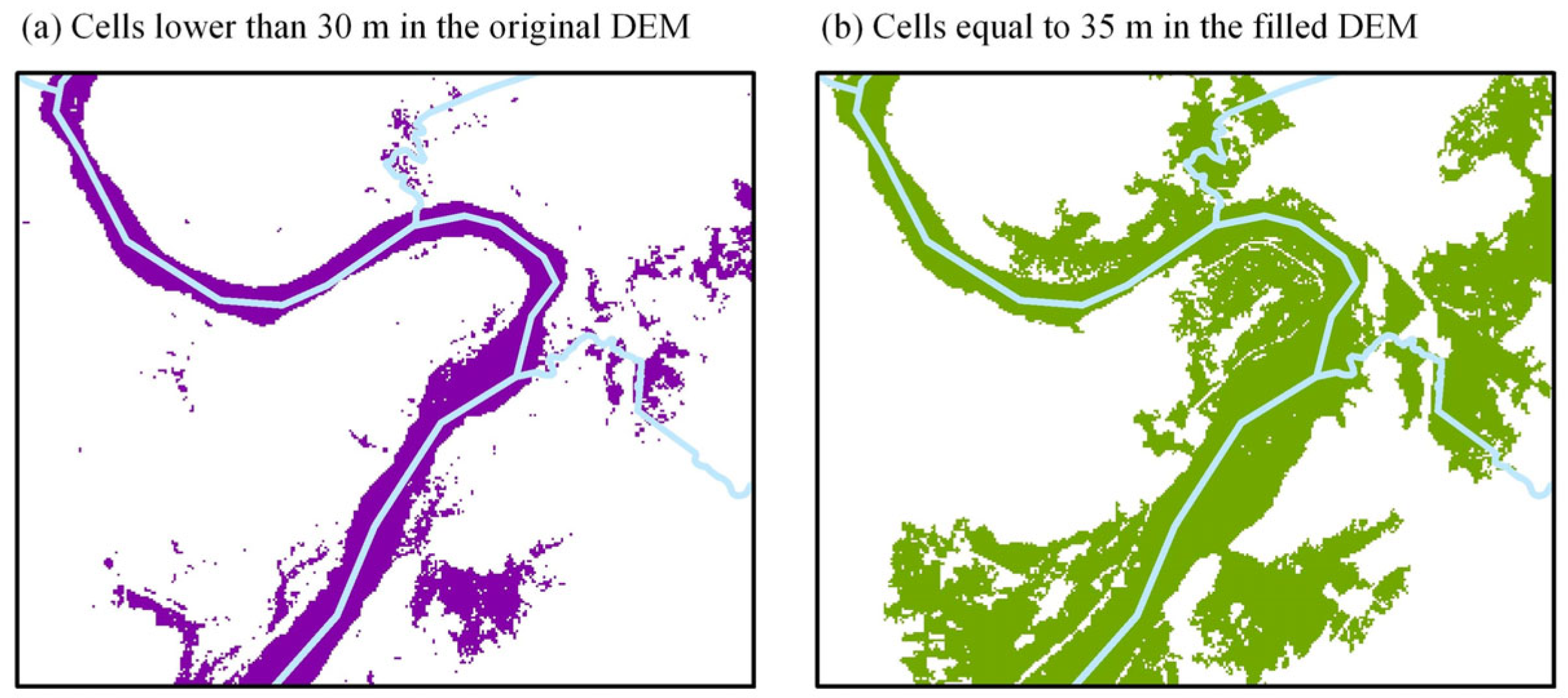
2.1. Issues in the Existing Algorithms

Algorithm 1 outlines the optimal framework of Priority-Flood proposed by Barnes et al. (2014) [27]. This framework is suitable for all kinds of DEMs, and PQ can be implemented by the implicit heap [31]. According to this framework, a stable PQ is created to order the inserted cells by ascending elevations. Initially, the cells on the terrain edges are defined as outlets and pushed into PQ. Then, the first cell, i.e., the lowest one, in PQ is popped out iteratively. Upon a cell being popped, each neighboring cell that has never been scanned is assigned a flow direction pointing to the popped cell and subsequently pushed into PQ. This process continues until no cell is left in PQ, and the whole drainage network is finally created. The procedure above contains all the necessary steps to implement the LCP algorithm, which is an improved version of Priority-Flood [26].

Algorithm 1 Pseudo-code of a framework for Priority-Flood algorithms. Upon input, DEM is an array storing the elevation for each cell. Upon output, FlowDirs is an array containing the flow direction assigned to each cell. Notably, if a cell in the array falls within the regions lacking valid elevation values, both DEM and FlowDirs assign it the value NoDATA. On line 8, a cell on terrain edges must be located at the outermost ring of the array or neighboring to a cell with the elevation value NoDATA

Require: DEM 1:   Let PQ be a stable priority queue sorting cells by ascending elevations; cells at the same elevation are arranged according to the insertion order. 2:   Let Closed and FlowDirs be matrices having the same dimensions with DEM. 3:   Initialize Closed to FALSE 4:   for all cell c 5:       if DEM[c] is NoDATA 6:           FlowDirs[c] ← NoDATA 7:           Closed[c] ← TRUE 8:       else if c is on the terrain edges 9:            PQ.push(c) 10:          Closed[c] ← TRUE 11:          Dir[c] ← Zero 12:  while PQ is not empty 13:       c ← PQ.pop() 14:       if c is not depression or flat 15:          call D8 algorithm for c        ◄ Only used by Wang and Liu (2006) [20] 16:       for all neighbors n of c           ◄ Cardinal neighbors first [27] 17:          if Closed[n] is FALSE 18:              FlowDirs [n] ← c 19:              Closed[n] ← TRUE 20:              if DEM[n] < DEM[c] 21:                  DEM[n] ← DEM[c]       ◄ Excluded by Metz et al. (2011) [26] 22:              PQ.push(n) 23:  return FlowDirs

In studies incorporating depression filling, the elevation of a newly scanned cell is modified to the higher value between its own elevation and that of the popped cell before inserting the new cell into PQ (line 21 in Algorithm 1). This modification provides the drainage network consistent with that extracted by Magalhães et al. (2014), although they used plain queues to replace the priority queue [21]. The flow direction assigned to a cell not in flats or depressions points to its lowest neighboring cell because PQ tends to pop lower cells first. Since the lowest neighbor may be not located at the steepest downstream direction [7], Wang and Liu (2006) recalculated the drainage directions with the D8 method for such cells (line 15 in Algorithm 1) [20].

Figure 1 demonstrates the influence of the cell insertion order in PQ when any existing Priority-Flood algorithm is applied to a flat. As shown in Figure 1a, the flat cells (white cells) at the same elevation are surrounded by higher cells (grey cells). Flat cells are required to drain to the outlet D1. If the neighboring cells of D1 are scanned clockwise from the north, C2 and D2 are inserted into PQ in sequence. When C2 is popped out, it receives the flow from D3 (Figure 1b). The extracted flow path from D3 (D3→C2→D1) is not the shortest route (D3→D2→D1). If the cells in cardinal directions are scanned earlier than those in diagonal directions, following the suggestion of Barnes et al. (2014) [27], the cells D2, C2, and D3 are popped from PQ in turn; then, the drainage network is generated (Figure 1c–e). Each flat cell is assigned the shortest flow path to the outlet in this example (Figure 1e). However, the existing algorithms ignore that the optimal zigzag flow path surrounding the straight theoretical route (yellow dashed arrow) should frequently twist [32]. The extracted flow path for C4 (Figure 1f) deviates from the optimal zigzag flow path (Figure 1g), although they have the same length. For an optimal result, the downstream flow path with more twists is preferred when determining the flow direction for a flat cell. This is hard to take into account when using the existing algorithms because the flow direction of a cell is determined as soon as it is scanned. Thus, a secondary correction should be added to the algorithm to optimize the flow paths.

A stable PQ is used to ensure that a flow path has the shortest length because it allows a cell closer to the outlet to have a higher priority when determining the drainage target for its neighboring cells. In fact, this aim can be achieved through another strategy, i.e., arranging cells at the same elevation in PQ according to their flow distances to the outlet of the flat. For cells sharing both the elevation and flow distance value, their orders in PQ are not important. Hence, a weak-ordering PQ with two priorities, i.e., elevation and flow distance, can be used to reduce the time consumed by ordering, but extra time is required to calculate and save the flow distance values. We couple such a weak-ordering PQ into the new algorithm and evaluate whether this approach can improve the efficiency significantly in Section 4.2.

2.2. Framework of the Improved Algorithm

In order to address the shortcomings of the existing Priority-Flood algorithms, a new algorithm is developed in this study. This new algorithm, which adds the flow Distance and the Zigzag pattern of the flow path as new parameters into the Priority-Flood theory, is named the DZFlood algorithm. The framework of DZFlood is modified from Algorithm 1, with optional depression filling.

To execute DZFlood, two parameters initialized as zero are attached to each cell, including the flow distance (FD) to the outlet as well as the number of continuous downstream cells sharing the same flow direction (NSD) before reaching the outlet. Notably, the outlet referenced by FD and NSD belongs to a flat, rather than the entire drainage network, as these parameters are designed for processing flat cells. As shown in Figure 1e, cell D4 has an FD of three times the cell size and an NSD of 2 because two continuous downstream flat cells (D3 and D2) have the same flow direction as D4. NSD reflects the zigzag degree of a flow path because a high NSD indicates a long straight segment and implies that a potential twist is needed. If a cell has at least one lower neighbor, it serves as an outlet of a flat, with FD and NSD set to zero, and its flow direction assignment will not be affected by these parameters. Additionally, a weak-ordering PQ with two priorities is created to sort cells by elevations (low to high). For cells with equal elevation, the one with the lower FD will be popped earlier from PQ. Cells with identical elevation and FD are randomly arranged in PQ.

Figure 2 illustrates the workflow of DZFlood without depression filling. Given a DEM (Figure 2a), cells on the terrain edges are assigned specific flow direction values for the drainage network outlets and pushed into PQ (Figure 2b). Here, any edge cell should be located at the outermost ring of the DEM or neighboring a cell without valid elevation. While the FDs of all edge cells are zero, the orders of these cells in PQ depend on their elevation (H in Figure 2). The arrangement of the cells with equal elevation and FD shown in Figure 2 is just a possible scenario due to the random arrangement of cells with equal priority in a weak-ordering PQ. But any arrangement cannot affect the results because no cell is allowed to drain to another cell with identical H and FD. Then, the first cell c in PQ is popped out one by one for computation.

Once c is popped, its flow direction is corrected following four cases:

Case 1: c is a drainage network outlet (e.g., D1 in Figure 2c). No correction happens.

Case 2: The downstream cell m (D1 in Figure 2d,e), pointed by the initial drainage direction of c (D2 in Figure 2d and C2 in Figure 2e), has a higher elevation than c. Then, no correction happens.

Case 3: The downstream cell m has the same elevation as c. In this case, each cell k neighboring both m and c is checked. If k also has the same elevation as c and Length(k,c) + FD(k) = FD(c), k is a potential drainage target of c that can also offer the shortest flow path for c. Here, the function Length(k,c) returns the distance between k and c. If k and c are cardinal neighbors, the distance is equal to the DEM resolution. If k and c are diagonal neighbors, the distance is $\sqrt{2}$ times the DEM resolution. Subsequently, five sub-cases are considered.

Sub-case 1: No potential target k is found. Then, the flow direction of c needs no correction (D3 in Figure 2f and D4 in Figure 2h). However, if the flow direction assigned to m is the same as the direction from c to m, let NSD(c) = NSD(m) + 1. For instance, c and m, respectively, represent D3 and D2 in Figure 2f; so, the NSD of D3 is 1 when the NSD of D2 is equal to 0.

Sub-case 2: The flow direction assigned to m is inconsistent with the direction from c to m, and the flow direction assigned to k is inconsistent with the direction from c to k. The cell with the lower NSD value is selected as the final drainage target for c (Figure 2i). If the NSDs of m and k are equal, the initial flow direction is retained (Figure 2g).

Sub-case 3: The flow direction assigned to m is consistent with the direction from c to m, and the flow direction assigned to k is consistent with the direction from c to k. The cell with the lower NSD value is selected as the drainage target for c. If the NSDs of m and k are equal, the initial flow direction is inherited. Then, the NSD(c) is renewed to 1 + NSD₁. NSD₁ is the lower value of the NSDs of m and k.

Sub-case 4: The flow direction assigned to m is consistent with the direction from c to m, and the flow direction assigned to k is inconsistent with the direction from c to k. In this sub-case, the flow direction of c is modified to point to k (Figure 2j).

Sub-case 5: The flow direction assigned to m is inconsistent with the direction from c to m, and the flow direction assigned to k is consistent with the direction from c to k. In this sub-case, the initial flow direction is retained (Figure 2k).

Case 4: If m is lower than c, each neighboring cell n of c is checked. The flow direction of c is modified to point to the neighbor that has been assigned a flow direction and owns the steepest slope (B5 in Figure 2l). Once multiple cells can cause the steepest slope, the first cell scanned is selected. The slope (S) is calculated as:

$$S=\left(H\left(c\right)-H\left(n\right)\right)/Length\left(c,n\right)$$

(1)

where H(c) and H(n) denote the elevation of c and n, respectively. For all the cases above, together with the flow direction modification, each neighboring cell n of c without a flow direction (e.g., C2 or D2 in Figure 2c) is given an initial flow direction pointing to c. Then, the FD of n is calculated as:

$$FD\left(n\right)=\left\{\begin{array}{cc}Length\left(n,c\right)\hfill & \hfill \mathrm{if} H\left(n\right)\ne H\left(c\right)\\ Length\left(n,c\right)+FD\left(c\right)\hfill & \hfill \mathrm{if} H\left(n\right)=H\left(c\right)\end{array}\right.$$

(2)

Subsequently, n is inserted into PQ according to its elevation and FD, and the first cell in PQ is popped for a new loop. Once there are no cells left in PQ, the whole drainage network is extracted for the DEM (Figure 2l). If depression filling is needed, the elevation of n should be raised to the elevation of c before pushing n into PQ if n is lower than c.

In the example in Figure 2, the flow path for D4 (i.e., C4→C3→D2→D1) extracted by DZFlood is the optimal one, as shown in Figure 1g. Similar to LCP, the time complexity of DZFlood is O(nlogn) due to the dominance of PQ on efficiency. To show the implementation of DZFlood more obviously, a pseudo-code is provided in Algorithm A1 (Appendix A), and the procedure of flow direction modification is listed as an independent function in Algorithm A2. The Java codes of DZFlood can be downloaded from Supplementary Materials.

3. Materials and Algorithms for Assessments

The performance of DZFlood is tested using the AW3D30 digital surface model with a resolution of 1″ (~30 m). The digital surface model can be treated as a normal DEM when assessing flow direction algorithms. The study area, located in southern China, covers a 5° × 5° region (113° E–118° E, 23° N–28° N) and has 18,000 × 18,000 cells (Figure 3a). There are many steep mountains with flat valleys and plains between them, resulting in an average slope of 16.1° (Figure 3b,c). The southeastern part of the study area is covered by the ocean (Figure 3c). Different from other DEMs that replace the ocean with invalid cells, AW3D30 assigns an elevation value of 0 m to the ocean. The ocean cells are preserved in this study, so a DEM with more valid cells can be used to assess the computation efficiency of different algorithms. Moreover, the existence of ocean cells will not affect the overland drainage network extraction because they are lower than land cells. Overall, flat cells with no downslope adjacent cell occupy 4.2% of all the cells in the DEM, and an extra 6.3% of all the cells will be converted to flat cells once the depressions are filled.

It is obvious that the sampling errors that exist in the DEM give some cells unrealistic elevations (e.g., −87 m for the lowest cell); therefore, flat and depression treatments are required for drainage network extraction. In order to assess the computation efficiency based on different cell numbers, four sub-regions with different areas (1° × 1°, 2° × 2°, 3° × 3°, 4° × 4°) are clipped from the DEM. Each sub-region has the point (113° E, 23° N) as the bottom left corner. The two locations marked in Figure 3a are selected for the visual assessments of extracted drainage networks, including Xinfengjiang Reservoir (114.5° E, 23.8° N) and a segment of Bei River (113.4° E, 24.3° N). Xinfengjiang Reservoir is the largest reservoir in southern China and has a large lake (Figure 3d). The selected segment of Bei River has a wide and flat valley (Figure 3e). These terrains are suitable for the assessment of algorithms focusing on flats or depressions. Furthermore, the water body dataset provided by OpenStreetMap is adopted for reference.

Five existing algorithms are selected to compare with DZFlood. The algorithm proposed by Wang and Liu (2006; referred to as the W&L algorithm) [20] and the LCP algorithm [24] are used to represent the existing Priority-Flood algorithms considering depression filling or not, respectively. The existing studies have not demonstrated the necessity of using a stable PQ, so the comparison also employs another version of LCP (referred to as LCP-WPQ), which adopts a weak-ordering PQ to replace the stable PQ used in LCP.

To create a height difference for neighboring flat cells when using the Priority-Flood theory to fill depressions, a DEM without flats and depressions can be efficiently generated with a weak-ordering PQ [27]. Algorithm 1 can be modified for this purpose by removing all flow direction assignment patterns and letting the neighboring depression/flat cell n of the popped cell c to be at least ε higher than c (i.e., DEM(n) = DEM(c) + ε on line 21 in Algorithm 1). Then, a gradient-based flow direction algorithm can be applied to the modified DEM for drainage network extraction. If the flow direction algorithm is sufficiently efficient, the time consumption may be lower than some Priority-Flood-based algorithms because of the difference between the computation efficiencies of the stable PQ and the weak-ordering PQ. In this study, ε is defined as 0.001 m, and the classical D8 algorithm is applied to the modified DEM. Moreover, since the precision of D8 is relatively low among gradient-based algorithms [32,33], the iFAD8 algorithm is selected as the representation of high-accuracy algorithms [32]. In fact, the flat/depression-removal method mentioned above has the same results as the depression-filling method suggested by D8 [7], but it is more efficient.

Overall, the performance of DZFlood is compared with those of W&L, LCP, LCP-WPQ, D8, and iFAD8 (

Table 1. Algorithms selected for assessments.

Name	Are Depressions Filled?	Type of PQ	Reference
D8	Yes	Weak-ordering	[7,27]
iFAD8	Yes	Weak-ordering	[27,32]
W&L	Yes	Stable-ordering	[20]
LCP	No	Stable-ordering	[26]
LCP-WPQ	No	Weak-ordering	[26]
DZFlood	No	Weak-ordering	This study

). Here, D8 and iFAD8 couple the PQ-based module of depression and flat removal. All the algorithms are implemented using Java 17 language, and they are tested on a computer equipped with an Intel(R) Xeon(R) E5-1620 v4 3.50 GHz CPU and 64 GB of memory.

4. Results and Discussion

4.1. Accuracy of the Extracted Drainage Networks

The two locations marked in Figure 3 are selected for visual assessments. In the DEM of the enlarged region covering the selected segment of Bei River, many small depressions (or so-called pits) exist, whose bottoms have an elevation lower than 30 m (i.e., the small independent purple points in Figure 4a), and the river cells of Bei River also have elevations lower than 30 m. The original intention of depression filling is to remove the small independent pits, but the river cells as well as some valley cells will be raised to 35 m at the same time because a block with an elevation of 35 m exists downstream (Figure 4b). Then, the extracted river is forced to cross the valley for a shorter flow distance. Thus, all the algorithms adopting depression filling (i.e., D8, iFAD8, and W&L) fail to extract drainage networks consistent with the real Bei River because depression filling removes valley topography from the DEM (Figure 5a–c). Some extra techniques, such as stream burning, can improve the performance [34], but they are not considered in this study because data other than the DEM are required. The drainage networks extracted by the three algorithms that ignore depression filling (i.e., LCP-WPQ, LCP, and DZFlood) closely match the real Bei River (Figure 5d–f). In the displayed area, DZFlood has the best performance (Figure 5f), whereas LCP-WPQ (Figure 5d) and LCP (Figure 5e) cannot correctly restore the southeast tributary. The results for Bei River prove that the preservation of depressions is significant for the description of earth surface processes (Figure 5a–f) [35]. Whether the depression covers a large area or a small independent pit, LCP-WPQ, LCP, and DZFlood never remove the depression structure from DEMs. They firstly concentrate the flow inside a depression to the depression bottom and then create an uplifted path to drain the flow outside from the lowest cell at the depression boundary [27]. This strategy can retain most of the natural paths, according to the results in Figure 5d–f.

Although depression filling has minimal impact on the elevations of the lake cells in Xinfengjiang Reservoir, D8, iFAD8, and W&L create many unreasonable parallel flow paths (Figure 5g–i). These shortcomings have been shown by several existing studies [12,36]. Overall, depression filling may not be the most suitable approach for terrains with relatively low relief. In addition, the difference between the drainage networks extracted by D8 and iFAD8 is small. Although iFAD8 is proven to have a better performance than D8 when applied to hillslopes or artifact terrains, the advantage is not obvious here because the artificial gradient attached to the flat is too low.

For Xinfengjiang Reservoir, the drainage network derived by LCP-WPQ appears disordered and contains some flow paths that are too long (Figure 5j). This phenomenon demonstrates that a stable PQ is crucial for producing simple and reasonable drainage networks when any traditional Priority-Flood algorithm is used. LCP and DZFlood provide acceptable results for Xinfengjiang Reservoir (Figure 5k,l), although LCP produces some overly straight river segments and abrupt twists. The flow distances from each flat cell to the outlet of the entire flat region are calculated based on the drainage networks extracted by LCP and DZFlood. It is found that the flow distance values of any flat cell derived by LCP and DZFlood are equal. However, the flow path derived by LCP may not surround the theoretical flow path, not limited by the raster format, as shown in Figure 1f, while the theoretical flow path is the practical shortest pathway.

Generally, LCP and DZFlood outperform the other algorithms in the visual assessments, and the drainage networks extracted by DZFlood are more consistent with the references provided by OpenStreetMap. The advantage of DZFlood over the flats, such as lakes, results from the consideration of zigzag routes. Moreover, DZFlood chooses the steepest downstream directions for most cells outside flats and depressions, while LCP simply routes the flow to the lowest neighboring cells. Although this difference does not cause obvious issues in Figure 5, the treatment chosen by DZFlood is undoubtedly better.

The strategies taken by DZFlood are compromises on computation efficiency, while some shortcomings still exist. For example, the outlet selected by DZFlood for any depression is the lowest boundary cell. This lowest cell may be affected by sampling errors and not located at a real valley. In further studies, where accuracy takes precedence over efficiency, some automatic methods for valley line extraction can be used to assist in the selection of outlet cells (e.g., [35,37]). Due to the high accuracy for low-relief regions, the flow direction derived by DZFlood is supposed to be suitable for applications in modelling overland flow and groundwater. However, according to DZFlood, the extracted flow path leading the flow to go outside a depression directs from low to high when the depression terrain is retained, while the real discharge is driven by the local downslope gradients [38,39]. Some significant hydraulic parameters, such as flow velocity, are calculated based on the downslope gradients. So, extra methods should be developed to provide reasonable hydraulic parameters for the uplifted flow paths in future studies.

4.2. Computation Efficiency

Figure 6 presents the runtimes required by different algorithms except for iFAD8 to process the DEMs of the whole study area and the four sub-regions described in Section 3. The runtime of iFAD8 is too inefficient for large-scale DEMs and shows no advantages over D8. For example, iFAD8 consumes 1328 s to process the 5° × 5° region. This runtime is at least 3 times those of the other algorithms and twice that of DZFlood. The D8 algorithm, coupled with a PQ-based module for depression and flat removal, has the highest efficiency. When only elevation is taken into account, the algorithms adopting a stable PQ (W&L and LCP) require significantly more time than those adopting a weak-ordering PQ (D8 and LCP-WPQ). The weak-ordering PQ employing both elevation and flow distance as priorities shows intermediate efficiency because it is unnecessary to sort cells with equal elevation and flow distance. The extra consideration of the zigzag flow path shape reduces the computation efficiency of DZFlood, while the use of a weak-ordering PQ improves the efficiency. Overall, the efficiency is improved, so DZFlood requires more runtime than D8 and LCP-WPQ but less runtime than W&L and LCP.

Since DZFlood and LCP have high accuracy in drainage network extraction, the difference between their efficiencies is important. For small-scale DEMs (e.g., 1.3 × 10⁷ cells in the 1° × 1° region), the runtime of DZFlood (13.9 s) is only 3.7% shorter than that of LCP (13.4 s) because calculating FDs and NSDs in DZFlood needs more time than the stable PQ ordering in LCP. As the number of cells increases, the runtime for the FD/NSD calculation increases linearly, while that for PQ sorting increases exponentially. When a large-scale DEM is used, the time saved by the weak-ordering PQ is more than the time consumed by the FD/NSD calculation. So, DZFlood consumes 19.2% less time than LCP on average, and a larger relative difference between their efficiency appears for a larger DEM. For the largest DEM with 3.24 × 10⁸ cells, DZFlood is 28.1% faster than LCP.

Future research could explore several promising approaches to further enhance the efficiency of DZflood. Firstly, by dividing a DEM into multiple tiles directly [13] or dividing the terrain into islands after flooding parts of the DEM [22], parallel computation can be used to process the sub-regions separately. Secondly, if an integer-type DEM is used, replacing only PQ with a list of plain queues or PQs may be able to save time for sorting cells [21]. However, further efforts are needed to realize the combination of DZFlood and the above technologies.

5. Conclusions

A new Priority-Flood algorithm named DZFlood is proposed, which simultaneously processes flats/depressions and extracts flow directions based on a DEM. The algorithm initializes by adding the cells on terrain edges into PQ; then, it iteratively removes the front cells while inserting the newly scanned cells, thereby generating complete flow paths draining to outlets. Different from the stable PQ used by the existing methods, a weak-ordering PQ with two priorities is adopted by DZFlood for the same results as the stable PQ but with lower time costs. In the dual-priority PQ, the lower cells are considered first, and a cell closer to the outlet has a higher priority than the other cells at the same elevation. For a flat cell with multiple potential downstream flow paths sharing the slowest flow distance, a secondary modification is applied to choose the most tortuous one.

The results demonstrate that depression filling may extremely change the terrains and prevent the river networks from being properly extracted. By preserving depression topography, DZFlood achieves optimal performance. Additionally, the computation efficiency of DZFlood is relatively high. Compared with LCP, DZFlood is 19.2% faster on average and has a higher relative efficiency for a larger DEM. When the DEM has 3.24 × 10⁸ cells, DZFlood is 28.1% faster than LCP. Hence, DZFlood has the potential to be applied to DEMs with massive cells.

References

1. Hickey, R. Slope Length Calculations from a DEM within ARC/INFO Grid. Comput. Environ. Urban Syst. 1994, 18, 365–380. [Google Scholar] [CrossRef]
2. Riihimäki, H.; Kemppinen, J.; Kopecký, M.; Luoto, M. Topographic Wetness Index as a Proxy for Soil Moisture: The Importance of Flow Routing Algorithm and Grid Resolution. Water Resour. Res. 2021, 57, e2021WR029871. [Google Scholar] [CrossRef]
3. Zhou, G.; Wei, H.; Fu, S. A Fast and Simple Algorithm for Calculating Flow Accumulation Matrices from Raster Digital Elevation. Front. Earth Sci. 2019, 13, 317–326. [Google Scholar] [CrossRef]
4. Tabunshchik, V.; Dzhambetova, P.; Gorbunov, R.; Gorbunova, T.; Nikiforova, A.; Drygval, P.; Kerimov, I.; Kiseleva, M. Delineation and Morphometric Characterization of Small- and Medium-Sized Caspian Sea Basin River Catchments Using Remote Sensing and GISs. Water 2025, 17, 679. [Google Scholar] [CrossRef]
5. Wilson, J.P.; Lam, C.S.; Deng, Y. Comparison of the Performance of Flow-routing Algorithms used in GIS-based Hydrologic Analysis. Hydrol. Process. 2007, 21, 1026–1044. [Google Scholar] [CrossRef]
6. Wu, P.; Liu, J.; Han, X.; Feng, M.; Fei, J.; Shen, X. An Improved Triangular Form-Based Multiple Flow Direction Algorithm for Determining the Nonuniform Flow Domain over Grid Networks. Water Resour. Res. 2022, 58, e2021WR031706. [Google Scholar] [CrossRef]
7. O’Callaghan, J.F.; Mark, D.M. The Extraction of Drainage Networks from Digital Elevation Data. Comput. Vis. Graph. 1984, 28, 328–344. [Google Scholar]
8. Khan, A.; Richards, K.S.; Parker, G.T.; McRobie, A.; Mukhopadhyay, B. How Large is the Upper Indus Basin? The Pitfalls of Auto-delineation using DEMs. J. Hydrol. 2014, 509, 442–453. [Google Scholar] [CrossRef]
9. Lindsay, J.B.; Creed, I.F. Removal of Artifact Depressions from Digital Elevation Models: Towards a Minimum Impact Approach. Hydrol. Process. 2005, 19, 3113–3126. [Google Scholar] [CrossRef]
10. Chen, B.; Ma, C.; Xiao, Y.; Gao, H.; Shi, P.; Zheng, J. Retaining Relative Height Information: An Enhanced Technique for Depression Treatment in Digital Elevation Models. Water 2021, 13, 3347. [Google Scholar] [CrossRef]
11. Jenson, S.K.; Domingue, J.O. Extracting Topographic Structure from Digital Elevation Data for Geographic Information System Analysis. Photogramm. Eng. Remote Sens. 1988, 54, 1593–1600. [Google Scholar]
12. Liu, Y.; Zhang, W.; Xu, J. Another Fast and Simple DEM Depression-Filling Algorithm Based on Priority Queue Structure. Atmos. Ocean Sci. Lett. 2009, 2, 214–219. [Google Scholar]
13. Barnes, R. Parallel Priority-Flood Depression Filling for Trillion Cell Digital Elevation Models on Desktops or Clusters. Comput. Geosci. 2016, 96, 56–68. [Google Scholar] [CrossRef]
14. Soille, P.; Gratin, C. An Efficient Algorithm for Drainage Network Extraction on DEMs. J. Vis. Commun. Image R. 1994, 5, 181–189. [Google Scholar] [CrossRef]
15. Nardi, F.; Grimaldi, S.; Santini, M.; Petroselli, A.; Ubertini, L. Hydrogeomorphic Properties of Simulated Drainage Patterns using Digital Elevation Models: The Flat Area Issue. Hydrolog. Sci. J. 2008, 53, 1176–1193. [Google Scholar] [CrossRef]
16. Martz, L.; Garbrecht, J. The Treatment of Flat Areas and Depressions in Automated Drainage Analysis of Raster Digital Elevation Models. Hydrol. Process. 1998, 12, 843–855. [Google Scholar] [CrossRef]
17. Su, C.; Wang, X.; Feng, C.; Huang, Z.; Zhang, X. An Integrated Algorithm for Depression Filling and Assignment of Drainage Directions over Flat Surfaces in Digital Elevation Models. Earth Sci. Inform. 2015, 8, 895–905. [Google Scholar] [CrossRef]
18. Barnes, R.; Lehman, C.; Mulla, D. An Efficient Assignment of Drainage Direction over Flat Surfaces in Raster Digital Elevation Models. Comput. Geosci. 2014, 62, 128–135. [Google Scholar] [CrossRef]
19. Liu, X.; Wang, N.; Shao, J.; Chu, X. An Automated Processing Algorithm for Flat Areas Resulting from DEM Filling and Interpolation. ISPRS Int. J. Geo-Inf. 2017, 6, 376. [Google Scholar] [CrossRef]
20. Wang, L.; Liu, H. An Efficient Method for Identifying and Filling Surface Depressions in Digital Elevation Models for Hydrologic Analysis and Modelling. Int. J. Geogr. Inf. Sci. 2006, 20, 193–213. [Google Scholar] [CrossRef]
21. Magalhães, S.V.G.; Andrade, M.V.A.; Franklin, W.R.; Pena, G.C. A Linear Time Algorithm to Compute the Drainage Network on Grid Terrains. J. Hydroinform. 2014, 16, 1227–1234. [Google Scholar] [CrossRef]
22. Gomes, T.L.; Magalhães, S.V.G.; Andrade, M.V.A.; Franklin, W.R.; Pena, G.C. Efficiently Computing the Drainage Network on Massive Terrains using External Memory Flooding Process. Geoinformatica 2015, 19, 671–692. [Google Scholar] [CrossRef]
23. Tahmasebi Nasab, M.; Zhang, J.; Chu, X. A New Depression-dominated Delineation (D-cubed) Method. for Improved Watershed Modelling. Hydrol. Process. 2017, 31, 3364–3378. [Google Scholar] [CrossRef]
24. Liu, K.; Song, C.; Ke, L.; Jiang, L.; Ma, R. Automatic Watershed Delineation in the Tibetan Endorheic Basin: A Lake-oriented Approach Based on Digital Elevation Models. Geomorphology 2020, 358, 107127. [Google Scholar] [CrossRef]
25. Yamazaki, D.; Baugh, C.A.; Bates, P.D.; Kanae, S.; Alsdorf, D.E.; Oki, T. Adjustment of a Spaceborne DEM for Use in Floodplain Hydrodynamic Modeling. J. Hydrol. 2012, 436–437, 81–91. [Google Scholar] [CrossRef]
26. Metz, M.; Mitasova, H.; Harmon, R. Efficient Extraction of Drainage Networks from Massive, Radar-based Elevation Models with Least Cost Path Search. Hydrol. Earth Syst. Sci. 2011, 15, 667–678. [Google Scholar] [CrossRef]
27. Barnes, R.; Lehman, C.; Mulla, D. Priority-flood: An Optimal Depression-filling and Watershed-labeling Algorithm for Digital Elevation Models. Comput. Geosci. 2014, 62, 117–127. [Google Scholar] [CrossRef]
28. Schiavo, P.; Riva, M.; Guadagnini, L.; Zehe, E.; Guadagnini, A. Probabilistic Identification of Preferential Groundwater Networks. J. Hydrol. 2022, 610, 127906. [Google Scholar] [CrossRef]
29. Zhang, H.; Yao, Z.; Yang, Q.; Li, S.; Baartman, J.E.M.; Gai, L.; Yao, M.; Yang, X.; Ritsema, C.J.; Geissen, V. An Integrated Algorithm to Evaluate Flow Direction and Flow Accumulation in Flat Regions of Hydrologically Corrected DEMs. Catena 2017, 151, 174–181. [Google Scholar] [CrossRef]
30. Liu, J.; Chen, X.; Zhang, X.; Hoagland, K.D. Grid Digital Elevation Model Based Algorithms for Determination of Hillslope Width Functions through Flow Distance Transforms. Water Resour. Res. 2012, 48, W04532. [Google Scholar] [CrossRef]
31. Luengo Hendriks, C. Revisiting priority queues for image analysis. Pattern Recogn. 2010, 43, 3003–3012. [Google Scholar] [CrossRef]
32. Wu, P.; Liu, J.; Han, X.; Liang, Z.; Liu, Y.; Fei, J. Nondispersive Drainage Direction Simulation based on Flexible Triangular Facets. Water Resour. Res. 2020, 55, e2019WR026507. [Google Scholar] [CrossRef]
33. Orlandini, S.; Moretti, G.; Corticelli, M.A.; Santangelo, P.E.; Capra, A.; Rivola, R.; Albertson, J.D. Evaluation of Flow Direction Methods against Field Observations of Overland Flow Dispersion. Water Resour. Res. 2012, 48, W10523. [Google Scholar] [CrossRef]
34. Lindsay, J.B. The Practice of DEM Stream Burning Revisited. Earth Surf. Process. Landf. 2016, 41, 658–668. [Google Scholar] [CrossRef]
35. Moretti, G.; Orlandini, S. Thalweg and Ridge Network Extraction from Unaltered Topographic Data as a Basis for Terrain Partitioning. J. Geophys. Res. 2023, 128, e2022JF006943. [Google Scholar] [CrossRef]
36. Yan, D.; Wang, K.; Qin, T.; Weng, B.; Wang, H.; Bi, W.; Li, X.; Li, M.; Lu, Z.; Liu, F.; et al. A Data Set of Global River Networks and Corresponding Water Resources Zones Divisions. Sci. Data 2019, 6, 219. [Google Scholar] [CrossRef]
37. O’Brien, G.R.; Wheaton, J.M.; Fryirs, K.; Macfarlane, W.W.; Brierley, G.; Whitehead, K.; Gilbert, J.; Volk, C. Mapping Valley Bottom Confinement at the Network Scale. Earth Surf. Process. Landf. 2019, 44, 1828–1845. [Google Scholar] [CrossRef]
38. Schiavo, M. Quantile-Based Approach for Improving the Identification of Preferential Groundwater Networks. Water 2025, 17, 282. [Google Scholar] [CrossRef]
39. Berkowitz, B.; Zehe, E. Surface Water and Groundwater: Unifying Conceptualization and Quantification of the Two “Water Worlds”. Hydrol. Earth Syst. Sci. 2020, 24, 1831–1858. [Google Scholar] [CrossRef]
Figure 1. Unreasonable flow paths may be extracted by any existing Priority-Flood algorithm for a flat region due to the cell insertion order in the priority queue (PQ). (a) The flat terrain is surrounded by higher wall cells and has only one outlet, i.e., D1. (b) If eight neighboring cells are scanned clockwise from the north and inserted into PQ following the same order, C2 is the first cell popped from PQ; then, cell D3 cannot obtain the shortest flow path to D1. (ce) Prioritizing cardinal over diagonal neighbors during scanning and inserting, D2, C2, and D3 are popped, in turn, from PQ; (f) then, the extracted flow path out from C4 is inconsistent with (g) the optimal zigzag one surrounding the straight line.
Water 17 01273 g001
Figure 2. An example of applying the DZFlood algorithm to a DEM with a 1 m resolution. (a) The cell elevation shows that the DEM contains a depression. A large flat region at an elevation of 4 is located in the depression. (b) Cells on the terrain edges are assigned the flow direction value of zero and pushed into the priority queue (PQ) for sorting. (ck) Then, the first cell in PQ is popped out one by one (i.e., the cells D1, D2, C2, B2, D3, C3, B3, D4, C4, B4, C5, and B5, in turn). A secondary correction is used to modify the flow direction of the popped cell; then, the neighboring cells that have never been scanned are assigned original flow directions and inserted into PQ. (l) Finally, the drainage network over the terrain is extracted. The flow distance (FD) from each cell to the outlet is reserved for one decimal place to show the results clearly.
Water 17 01273 g002
Figure 3. (a) The DEM, (b) the distribution of the local slope, and (c) a satellite image of the study area adopted for assessments. Two sub-regions in the study area are selected for visual assessments of the extracted drainage network, including (d) Xinfengjiang Reservoir and (e) a segment of Bei River.
Water 17 01273 g003
Figure 4. Distribution of river cells in (a) the original DEM (purple points) and (b) the filled DEM (green points) at Bei River. The blue lines are real rivers according to the OpenStreetMap dataset.
Water 17 01273 g004
Figure 5. The drainage networks extracted by different algorithms are marked by different colors for (af) a segment of Bei River and (gl) Xinfengjiang Reservoir. Each drainage network is defined based on the least contributing area of 30,000 cells. The blue regions in the background are real water bodies provided by the OpenStreetMap dataset.
Water 17 01273 g005
Figure 6. The runtimes consumed by different flow direction algorithms when DEMs of five scales are applied. Each runtime is averaged over 5 runs.
Water 17 01273 g006