Energy Cost Optimisation in a Wastewater Treatment Plant by Balancing On-Site Electricity Generation with Plant Demand

Abstract

Wastewater treatment plants (WWTPs) consume a considerable amount of energy. They also generate energy in combined heat and power (CHP) units, which utilise biogas from the anaerobic digestion of sewage sludge to produce renewable electricity. Different prices apply to electricity generated on site in CHP units, to the purchase of electricity from the grid, to the sale of surplus electricity to the grid and energy tariffs, which motivates the optimisation of energy costs. This paper presents a strategy for optimising electricity costs by adapting on-site electricity generation in CHP units to the demand of the WWTP. The approach is designed for a CHP system that generates electricity in multiple internal combustion gas engines. It is implemented as a two-level control system, where the lower control level dynamically adjusts the power of the individual gas engines, and the upper control level optimises the desired total power, taking into account the current energy consumption of the WWTP, biogas reserves and electricity tariffs. The proposed concept was implemented at the Domžale-Kamnik WWTP. A six-month evaluation showed that electricity purchased from the grid could be reduced from 8.7% to 3.3% of the WWTP’s electricity consumption. This reduction affects the system economically, as electricity purchased from the grid at low and high tariffs is 35% and 76% more expensive than electricity generated on site (excluding the grid fee). This approach can be extended to balance dispatchable electricity generation at the WWTP to respond to short-term grid demand.

1. Introduction

Wastewater treatment plants (WWTPs) consume a considerable amount of energy, estimated at 1% to 3% of global energy production [1]. They can also recover energy from the organic matter entrapped in wastewater by producing biogas from sewage sludge in anaerobic digestion and generating renewable electricity in biogas cogeneration units [2].

Traditional challenges associated with energy use in WWTPs include reducing energy consumption and increasing the production of renewable energy. A literature review examining global practices implemented across all stages of WWTP treatment processes to reduce energy consumption is provided in [3]. Methods to reduce energy consumption and increase energy recovery to achieve energy neutrality in WWTPs are presented in [4]. Most of the energy consumption is due to aeration. Therefore, aeration optimisation and control are of particular interest [5,6,7].

Another challenge is the reduction in energy costs. This includes energy cost optimisation based on energy tariffs. The flexibility of WWTPs to distribute the aeration load to periods with less expensive energy prices was studied in [8]. Different reject water scheduling control strategies were analysed on a benchmark simulation model to mitigate peak energy demand and optimise energy costs under alternative electricity tariff structures [9]. The importance of incorporating realistic energy cost models for energy cost optimisation has been demonstrated in [10]. This study presented a detailed energy cost model and showed the importance of considering energy tariffs when developing operational and control strategies. Ref. [11] studied how the diurnal cycles and peaks of the grid electricity tariffs coincide with peaks of influent load and electricity demand of a large WWTP in California, having an amplifying effect on the plant’s electricity costs and carbon footprint.

Recent challenges also consider the energy flexibility in WWTPs. This flexibility involves adapting grid electricity demand and supply to account for the fluctuating supply in a renewable electricity grid. The role of WWTPs in a future low-carbon electricity grid was investigated in [12]. This study analysed the flexibility of electricity generation and demand in WWTPs. Demand-side flexibility was achieved by load shifting, with 50% of the WWTP’s total electricity demand being shiftable. Supply-side flexibility was achieved by flexible electricity generation in biogas CHP (combined heat and power) units. The evaluation was performed by simulating a fully renewable electricity grid in Australia and modelling the nationwide electricity demand at WWTPs. The study concluded that WWTPs have significant potential for energy flexibility in a renewable energy grid.

A similar simulation study at national level was conducted in Ireland [13]. This study assessed the benefits of integrating 15 large-scale WRRFs (Water Resource Recovery Facilities) in Ireland into a future highly renewable smart-energy system through economic dynamic dispatch. This study analysed different options for electricity and heat generation, storage and recovery at the WWTP. These included, among others, anaerobic digestion, dynamic CHP electricity generation, electricity export to the grid and biogas storage. The study showed that the implementation of these scenarios reduced the aggregated annual costs of the overall system. Recently, ref. [14] presented an integrated energy-water model for the power system and the Irish wastewater sector. The aim was to assess the flexibility of air and water pumping to enable demand response capabilities in WWTPs. These two studies have shown that increased demand flexibility leads to a reduction in electricity costs, but process constraints of the WWTP processes impede the flexibility potential and need to be taken into account.

Several studies have been performed also with regard to flexible biogas and electricity production in WWTPs. Ref. [15] investigated the potential of dynamic biogas production from the anaerobic digestion of sewage sludge supported by specific feeding regimes for on-demand electricity generation. This study showed that demand-driven biogas production is operationally feasible and commercially advantageous compared to steady generation. Ref. [16] considered biogas plants with surplus generator capacity and gas storage. This study presented a method for maximising the profit of biogas plants in day-ahead unit commitment when participating in short-term electricity and control reserve markets. Ref. [17] investigated the dynamic characteristics of biogas plants with CHP systems to be used as a controllable power source for supply-demand adjustment in the power grid. This study investigated real-world biogas CHP systems in Germany and Japan and evaluated their start-up, shutdown and step response characteristics as well as their environmental impact, i.e., exhaust gas emissions during transient operation. The results showed that CHP systems have the potential to contribute to a long-term adjustment of power equivalent. However, they require several minutes between starting and stopping.

The above articles present analyses or simulation studies that examine the potential of WWTPs for flexible energy production and consumption, as well as energy trading within renewable energy grids. The general conclusion is that such potential does exist. However, as mentioned in [18], the research remains purely theoretical. Similar findings were reported in [19], emphasising that research on full-scale WWTPs is still limited.

One of the few studies performed at full-scale WWTPs is presented in [19]. In this study, three energy load-shifting strategies were investigated on a full-scale WWTP in California to examine how effectively the WWTP could participate in a demand response program. The strategies tested included the following: (i) shifting the timing of CHPs for energy generation, (ii) diverting flow equalisation basins to reduce system-wide energy use, and (iii) discharging an onsite battery. The test included eighteen test events. The study showed that the WWTP was able to shift its energy load without impacting WWTP effluent quality. The two main issues identified were the difficulty in properly timing the demand reduction periods and the inaccuracy in measuring the energy load reduction. The study estimated a potential cost reduction of 4.8% by participating as a demand resource in the energy market.

Another full-scale evaluation is presented in [18]. This study outlines a systematic approach to identify, evaluate, and safely implement typical aggregates (e.g., aerators, pumps, agitators, etc.) in WWTPs in order to enable flexible plant operation. This approach was initially developed and tested at a pilot WWTP in Germany, further refined by simulation and validated by field tests at three WWTPs. The result includes a list of potential aggregates along with their switch-on, switch-off and regeneration times that provide flexibility in energy consumption while ensuring effluent quality. The study confirmed flexibility in both energy generation and energy consumption in WWTPs to compensate for fluctuating renewable energy generation. However, the conclusions from this study highlighted that participation in the energy markets is not yet attractive enough for plant and grid operators due to the low economic benefits.

Based on the review above, it can be concluded that a significant research gap exists in examining full-scale WWTPs’ flexibility in adapting their energy consumption and generation patterns. CHP units are considered a good opportunity to gain initial experiences with interactions in the energy markets on the basis of existing operational knowledge in reducing external energy demand [18]. To implement such a strategy, a control system has to be designed and implemented at WWTPs, ensuring that the CHP units follow the desired set-point of total electricity generation while considering WWTP process constraints.

Thus, this paper focuses on flexible electricity generation and optimisation of energy costs in a full-scale WWTP with a biogas cogeneration unit. Cost optimisation is achieved by matching the electricity supply and demand within the WWTP and generating surplus electricity at a high energy tariff. The task is to develop a technical solution for balancing electricity supply and demand within the plant to achieve self-sufficient electricity generation, near-zero grid energy consumption and optimisation of energy costs. The solution presented dynamically adjusts the power of the biogas engines and controls the volume of biogas in the storage tank, taking energy tariffs into account. The system was implemented at the Domžale-Kamnik WWTP in Slovenia, where its performance was evaluated during six months of operation. Future studies may consider extending the system to balance the dispatchable electricity generation at the WWTP to respond to short-term grid demand.

This paper is organised as follows. In the next section, we first present the WWTP case study and the electricity price. Then, we present the concept of balancing the electricity demand and supply within the WWTP and its implementation details. In Section 3, we demonstrate the proposed concept on a full-scale WWTP and discuss the results. The paper ends with the conclusions and perspectives for future work.

2. Materials and Methods

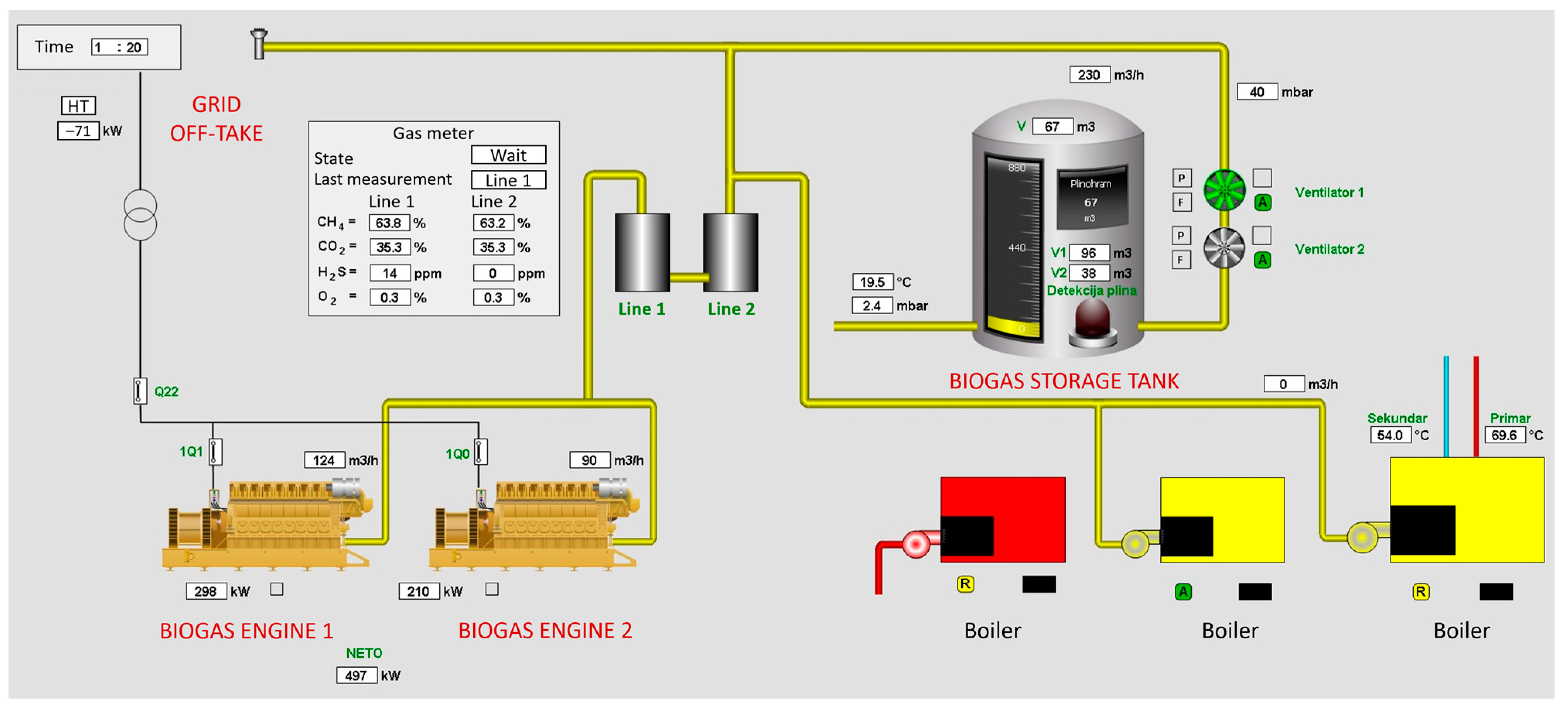
2.1. Case Study

The study considers a WWTP that treats municipal and industrial wastewater with a biological activated sludge process (Sequencing Batch Reactor technology, SBR) and carries out sludge treatment in an anaerobic digester. The current plant operating capacity is 100,000 population equivalents (PE). Biogas from the anaerobic digestion of sewage sludge and the co-digestion of organic waste is converted into renewable electricity using biogas engines (generators). Electricity and heat are generated by two generators, G1 and G2, with a maximum output electrical power of 300 kW and 210 kW, respectively (Figure 1). The generators run exclusively on biogas produced at the WWTP and no additional gas is supplied.

In 2023, on-site electricity generation from biogas covered 107.1% of the energy requirements for wastewater treatment. This means that on-site electricity generation exceeded the demand for the wastewater and sludge treatment. However, the plant is not completely self-sufficient in terms of electricity supply. Occasionally, because of the varying electricity demand of the technological processes and varying electricity supply from the biogas engines (e.g., fluctuating biogas production, limited power of the biogas engines and constraints on engine operation), the plant operates by taking the deficit of energy from the grid and supplying the surplus of generated electricity to the grid.

2.2. Energy Price

Depending on the current WWTP electricity demand and the on-site generated electricity, the WWTP can use the on-site generated electricity for its own needs, buy the electricity shortfall from the grid or sell the surplus production to the grid. The motivation for optimising energy costs is the price of energy in these different cases.

Different tariff structures are used for the grid electricity price in different countries based on the energy price structure (e.g., time-of-use rates) and charges (e.g., energy usage, peak power demand charges) [10,20]. In our case, the grid electricity price is based on a low and high tariff depending on the time of day.

Table 1. Electricity prices at the WWTP for grid purchase and sale to the grid compared to on-site generated electricity in biogas engines.

Grid Electricity Purchase/Sale Compared to On-Site Generation	Low Tariff	High Tariff 1
Grid purchase	35% + grid fee	76% + grid fee
Sales to grid	−18%	22%

Note: ¹ The high tariff applies on working weekdays from 6 a.m. to 10 p.m.

shows the prices for grid purchase and sale compared to the price of on-site generated electricity at high and low tariffs. The prices apply to this case study in 2024 and 2025. Buying energy from the grid at the high tariff is 76% more expensive than the electricity generated at the WWTP, while buying it at the low tariff is 35% more expensive (not including the grid fee). The price of electricity supplied to the grid is 22% higher at the high tariff than the electricity generated on-site, while it is 18% lower at the low tariff. In order to optimise the plant’s electricity costs, it is necessary to cover the WWTP electricity demand by the on-site generated electricity at the high tariff, to buy the electricity deficit at the low tariff and to generate the electricity surplus during the high tariff. Given the prices in Table 1, it is not reasonable to maximize electricity generation and sell the electricity to the grid at the high tariff at the expense of purchasing the electricity shortfall during the low tariff.

2.3. The Concept of Electricity Demand-Supply Balancing

The strategy for optimising energy costs is based on the dynamic adjustment of on-site electricity generation to electricity demand and the production of surplus electricity at a high tariff. The power generation is adjusted by dynamically changing the output of the biogas engines (CHP generators).

The technical solution for demand-supply management consists of a two-level control algorithm (Figure 2). The upper control level determines the desired total output power of the generators. The total output equals the current electricity demand of the plant but also considers the energy tariff and the available biogas storage. The lower-level control then adjusts the output power of the individual generators accordingly in order to achieve the desired total power.

The advantage of the proposed concept is that the power settings of the individual generators are always unique, relying solely on the desired total power and remaining independent of additional optimisation requirements. Those requirements (e.g., energy tariffs, gas reserves in the storage tank, shutdown delay of generators, etc.) can be considered by adjusting the desired total power of generators. In this way, the operation is more transparent and easier to manage.

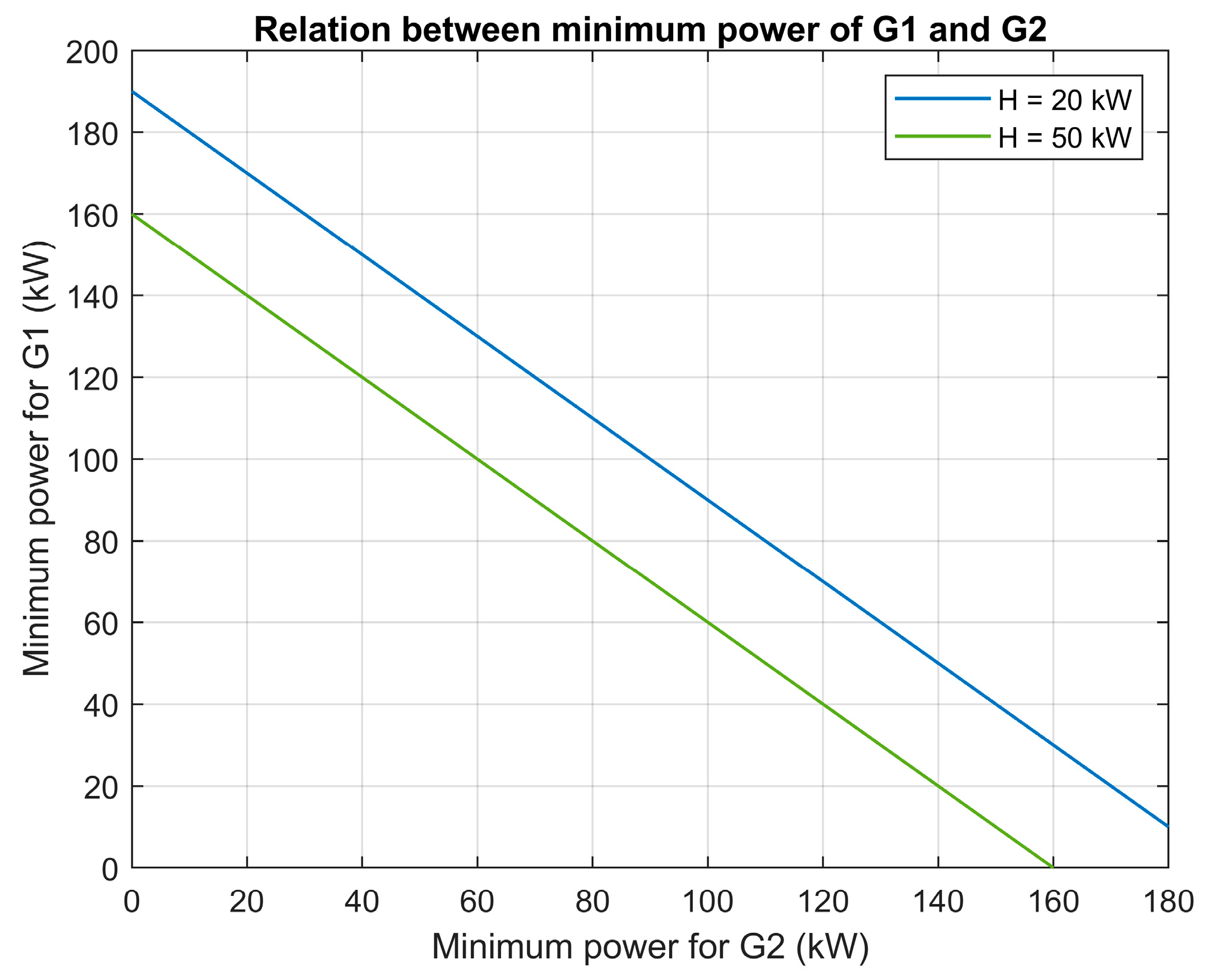
2.3.1. Setting the Generators’ Power

A power unit can operate with several CHP generators operating in an on/off mode or in partial load mode. Partial load means operation at a reduced capacity utilization level. CHP systems usually have a limited minimum possible partial load, typically above 50%. To adjust the power output of the generators, an electric load-tracking control strategy is used [21]. The focus is on adjusting the power output of the individual generators to follow the total power set-point and maximise the efficiency of the generators.

Consider a situation with two generators: to achieve a total power as close as possible to the desired value, the power of the individual CHP units must be adjusted. This means that at low total power, one (primary) generator is in operation and adjusts the operating power, while at high total power, two generators (primary and secondary) are in operation. To allow for a sudden increase/decrease in power when switching on/off the secondary generator, the step change in power due to minimum partial load must be compensated with a decrease/increase in the primary generator power. To achieve a smooth transition, the operating range of each generator must be at least as wide as the minimum power of the other generator. This applies regardless of which of the two generators is the primary one. In addition, the power range should be larger for an additional power representing a hysteresis that prevents the secondary generator from switching on and off too frequently. The constraints on the minimum power of each generator are as follows

$$P_{1\mathrm{m}\mathrm{i}\mathrm{n}}\le P_{2\mathrm{m}\mathrm{a}\mathrm{x}}-P_{2\mathrm{m}\mathrm{i}\mathrm{n}}-H,$$

(1)

$$P_{2\mathrm{m}\mathrm{i}\mathrm{n}}\le P_{1\mathrm{m}\mathrm{a}\mathrm{x}}-P_{1\mathrm{m}\mathrm{i}\mathrm{n}}-H,$$

(2)

where $P_{1\mathrm{m}\mathrm{i}\mathrm{n}}$, $P_{2\mathrm{m}\mathrm{i}\mathrm{n}}$, $P_{1\mathrm{m}\mathrm{a}\mathrm{x}}$ and $P_{2\mathrm{m}\mathrm{a}\mathrm{x}}$ are the minimum and maximum power of each generator and $H$ is the hysteresis power. Hysteresis is added to reduce the number of times the generators are switched on and off. If inequalities (1)–(2) hold, the ideal power characteristic curve can be obtained in the entire range between the minimum power of the primary generator and the sum of the maximum powers of both generators.

For the present case study with $P_{1\mathrm{m}\mathrm{a}\mathrm{x}}=300$ kW and $P_{2\mathrm{m}\mathrm{a}\mathrm{x}}=210$ kW, we obtain the following boundary conditions for the minimum power

$$P_{1\mathrm{m}\mathrm{i}\mathrm{n}}\le 210-P_{2\mathrm{m}\mathrm{i}\mathrm{n}}-H,$$

(3)

$$P_{2\mathrm{m}\mathrm{i}\mathrm{n}}\le 300-P_{1\mathrm{m}\mathrm{i}\mathrm{n}}-H.$$

(4)

If we express $P_{1\mathrm{m}\mathrm{i}\mathrm{n}}$ from (4), we obtain

$$P_{1\mathrm{m}\mathrm{i}\mathrm{n}}\le 300-P_{2\mathrm{m}\mathrm{i}\mathrm{n}}-H.$$

(5)

Since the inequality (3) is more severe than (5), we can transform (3) into equation

$$P_{1\mathrm{m}\mathrm{i}\mathrm{n}}=210-P_{2\mathrm{m}\mathrm{i}\mathrm{n}}-H.$$

(6)

For a desired $H$ and a chosen $P_{2\mathrm{m}\mathrm{i}\mathrm{n}}$, we can determine $P_{1\mathrm{m}\mathrm{i}\mathrm{n}}$ from (6) and vice versa. Figure 3 shows the possible combinations of $P_{1\mathrm{m}\mathrm{i}\mathrm{n}}$ and $P_{2\mathrm{m}\mathrm{i}\mathrm{n}}$ for two choices of $H$. It can be seen that in the case of $H=20$ kW, the highest minimum power for both generators is obtained at $P_{1\mathrm{m}\mathrm{i}\mathrm{n}}=P_{2\mathrm{m}\mathrm{i}\mathrm{n}}=95$ kW, and in the case of $H=50$ kW at $P_{1\mathrm{m}\mathrm{i}\mathrm{n}}=P_{2\mathrm{m}\mathrm{i}\mathrm{n}}=80$ kW. If choosing different values for the minimum power, then the $P_{1\mathrm{m}\mathrm{i}\mathrm{n}}$ is lower at higher $P_{2\mathrm{m}\mathrm{i}\mathrm{n}}$, and vice versa. The increase in the minimum power can only be achieved in the following cases: (i) if two generators with equal power are used, (ii) if the hysteresis is reduced, (iii) if the generator with higher maximum power is used as the primary generator.

In our case, the minimum values of the generators are $P_{1\mathrm{m}\mathrm{i}\mathrm{n}}=150$ kW and $P_{2\mathrm{m}\mathrm{i}\mathrm{n}}=120$ kW, and they do not fulfil the conditions to achieve an ideal total power curve. Therefore, the only option is to deviate from the ideal case. This means that in some cases the generators will not be able to deliver the desired total power over the entire characteristic curve.

Figure 4 shows two situations with generators G1 and G2 as primary generators. The algorithm for setting the power for each generator is shown in Supplementary Material S1. In the case of G1 as the primary generator, inequality (2) holds for $H\le 30$ kW. Therefore, by selecting $H=30$ kW, the ideal characteristic curve is obtained over the entire range between the minimum power of G1 and the sum of the maximum powers of both generators (Figure 4, left). In the case of G2 as the primary generator, inequality (1) fails for any positive hysteresis value and the target total power cannot be fully achieved (Figure 4, right). The deviation occurs when the total power set-point is between $P_{2\mathrm{m}\mathrm{a}\mathrm{x}}$ and $P_{1\mathrm{m}\mathrm{i}\mathrm{n}}+P_{2\mathrm{m}\mathrm{i}\mathrm{n}}$. By selecting $H=30$ kW and adjusting the switch-on and switch-off conditions for the secondary generator (see algorithm in Supplementary Material S1), the maximum theoretical error is 45 kW, which corresponds to up to 20% of the desired total power. Since exact tracking of the actual consumption by the CHP system is not required, the solution presented is considered sufficient. Note that G1 cannot always be the primary generator, as both generators must have a similar number of working hours.

The time delay between switching the secondary generator on and off is already implicitly solved by a given hysteresis $H$. In addition, the set-point for the total power can be supplemented by a rate limit to ensure that the total power does not change at a higher rate than the specified limit. The rate limit $v_P$ can be determined based on the hysteresis $H$, so that the secondary generator is not switched on and off in less than a minimum time $t_{min}$

$$v_P={\displaystyle \frac{H}{t_{min}}}.$$

(7)

Applying a rate limit to the total power set-point could slow down the power management of the generators, resulting in a higher deviation between power demand and generation. However, it also has the positive effect of reducing the rate of change in the generator power.

Another way to prevent generators from switching on and off frequently is to use a time limiter. It requires the implementation of a timer and additional switching conditions and is less transparent from a control point of view. The third option is to apply a sufficiently long sampling time of the algorithm, e.g., 5–10 min.

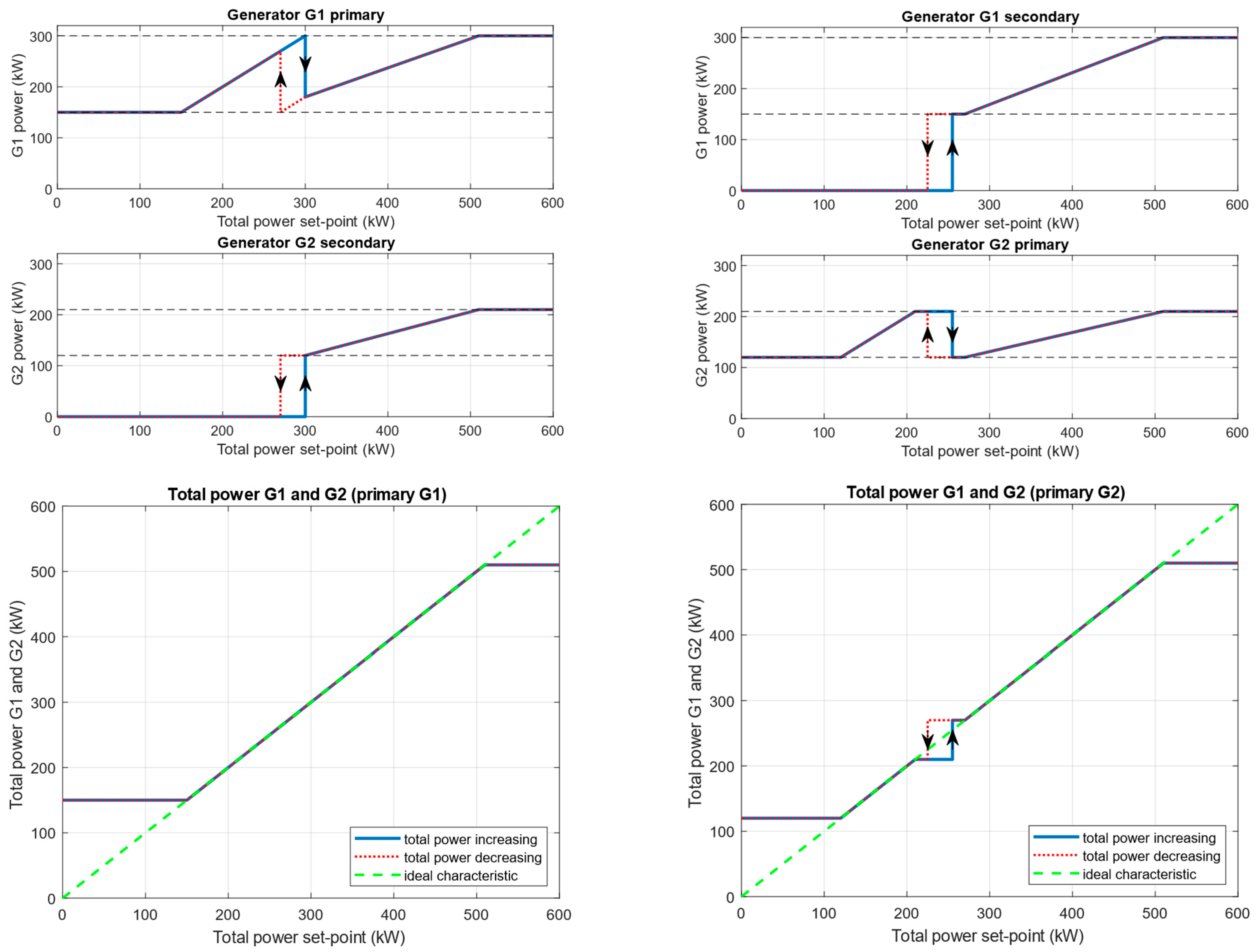
2.3.2. Determination of the Total Power Set-Point

When determining the desired total power, various optimisation requirements and constraints can be taken into account, which are presented below.

The desired total power $P_{ref}$ can be dynamically adjusted to the current electricity demand $P_{demand}$

$$P_{\mathit{ref}}=P_{demand}.$$

(8)

If the electricity generation capacity is sufficient to meet the demand, this gives the best result when optimising electricity costs given the energy prices for grid purchase, grid sale and on-site electricity generation in CHP units (Table 1).

If the on-site generation capacity is lower than the demand, a reasonable solution is to fully cover the demand during the high tariff and buy the electricity deficit during the low tariff. If, on the other hand, the electricity generation capacity exceeds the demand, it makes sense to meet the demand during the low tariff and generate the surplus electricity during the high tariff. These requirements can be taken into account by multiplying the current electricity demand by a factor $k_E$, which is set differently for high and low tariffs

$$P_{\mathit{ref}}={k_{E}P}_{demand}.$$

(9)

$k_E$ is set higher in the high tariff than in the low tariff. This ensures that more energy is always generated in the high tariff and less in the low tariff. If the electricity generation capacity is lower than the demand, $k_E$ is set to 1 in the high tariff and <1 in the low tariff. In the case of excess electricity generation capacity, $k_E$ is set to 1 in the low tariff and >1 in the high tariff.

For the smooth operation of the generators, it is necessary to ensure sufficient biogas storage in the storage tank. The volume of biogas should not be too low to interrupt the operation of the biogas engine or too high to require the combustion of excess biogas on the gas flare. The adjustment of the generator power to these requirements can also be implicitly taken into account by adjusting the total power set-point.

The biogas storage tank can hold gas quantities from 0 to $V_{max}$. $\mathsf{\Delta }V$ is used to define a normal operating range between low $V_L$ and high $V_H$ volume (Figure 5). If the current gas volume $V$ is within this range, the set-point for the total power is determined according to (9). If the volume falls below the low limit (${V<V}_L$), it is necessary to reduce the desired power of the generators accordingly. On the other hand, if the volume is higher than the high limit (${V>V}_H$), the desired power of the generators should be increased. If the volume is below $V_L$ or above $V_H$, the adjusted total power set-point $P_{ref}^{*}$ can be determined as follows

$$P_{\mathit{ref}}^{*}=P_{ref}-k_P{\displaystyle \frac{V_L-V}{\mathsf{\Delta }V}}, \mathrm{f}\mathrm{o}\mathrm{r} V<V_L,$$

(10)

$$P_{\mathit{ref}}^{*}=P_{ref}+k_P{\displaystyle \frac{V-V_H}{\mathsf{\Delta }V}}, \mathrm{f}\mathrm{o}\mathrm{r} V>V_H,$$

(11)

where $P_{ref}$ is determined in (9), and $k_P$ is an adjustable parameter. Equations (10) and (11) are intended to ensure that the gas storage tank is not completely emptied or filled. For example, the setting $k_P=P_{1\mathrm{m}\mathrm{a}\mathrm{x}}+P_{2\mathrm{m}\mathrm{a}\mathrm{x}}$ ensures that when the storage tank is almost empty, the calculated $P_{ref}^{*}$ is (below) zero and the generators are switched off. On the contrary, when the storage tank is almost full, $P_{ref}^{*}$ is above the sum of the maximum power of both generators.

2.4. Implementation

The proposed concept for balancing electricity demand and supply was implemented on a PLC and SCADA system at the Domžale-Kamnik WWTP. It was slightly adapted to this case study. In addition to the gas volume requirements described in Section 2.3.2, the pressure in the storage tank was also taken into account. Both conditions were taken into account by defining four different operating modes and different conditions for the transitions between these modes.

The final control algorithm consists of two state machines, one for the low tariff (L) and one for the high tariff (H). A scheme that applies to each state machine is shown in Figure 6. A state machine has four operating modes (states) that define the operating status of the generators, i.e., (1) primary generator operates at constant power, (2) primary generator adjusts power, (3) primary and secondary generators adjust power, (4) primary and secondary generators operate at maximum power. The conditions for the transitions between the states are defined on the basis of the gas volume and the pressure in the storage tank. In states L2/H2 and L3/H3, the output of the generators is adjusted by the algorithm presented in Supplementary Material S1, taking into account the number of generators in operation.

All setting parameters of the control algorithm are displayed in the SCADA system and can be set by the operator. A list of parameters and an example of their setting can be found in

Table 2. Parameters of the implemented control algorithm that can be adjusted in the SCADA system and an example of their settings.

Parameters of the Implemented Control Algorithm
Volume transitions
L1 to L2	>30%	L2 to L1	<10%
L2 to L3	>85%	L3 to L2	<15%
L3 to L4	>95%	L4 to L3	<90%
H1 to H2	>20%	H2 to H1	<10%
H2 to H3	>50%	H3 to H2	<15%
H3 to H4	>95%	H4 to H3	<90%
Pressure transitions
Any state to L4 (or H4)	>2.5 mbar
L4 to L3	<1.6 mbar	H4 to H3	<1.6 mbar
L3 to L2	<0.8 mbar	H3 to H2	<0.8 mbar
Time for pressure transitions
Any state to L4 (or H4)	2 min
L4 to L3 (or H4 to H3)	10 min
L3 to L2 (or H3 to H2)	15 min
Transition delay to a new state
Any state	15 min
Factor kE
Low tariff	1.0
High tariff	1.1

. Note that the conditions for transitions between operating modes are set for each state machine and may be different for low and high tariffs. An example of an operation is as follows:

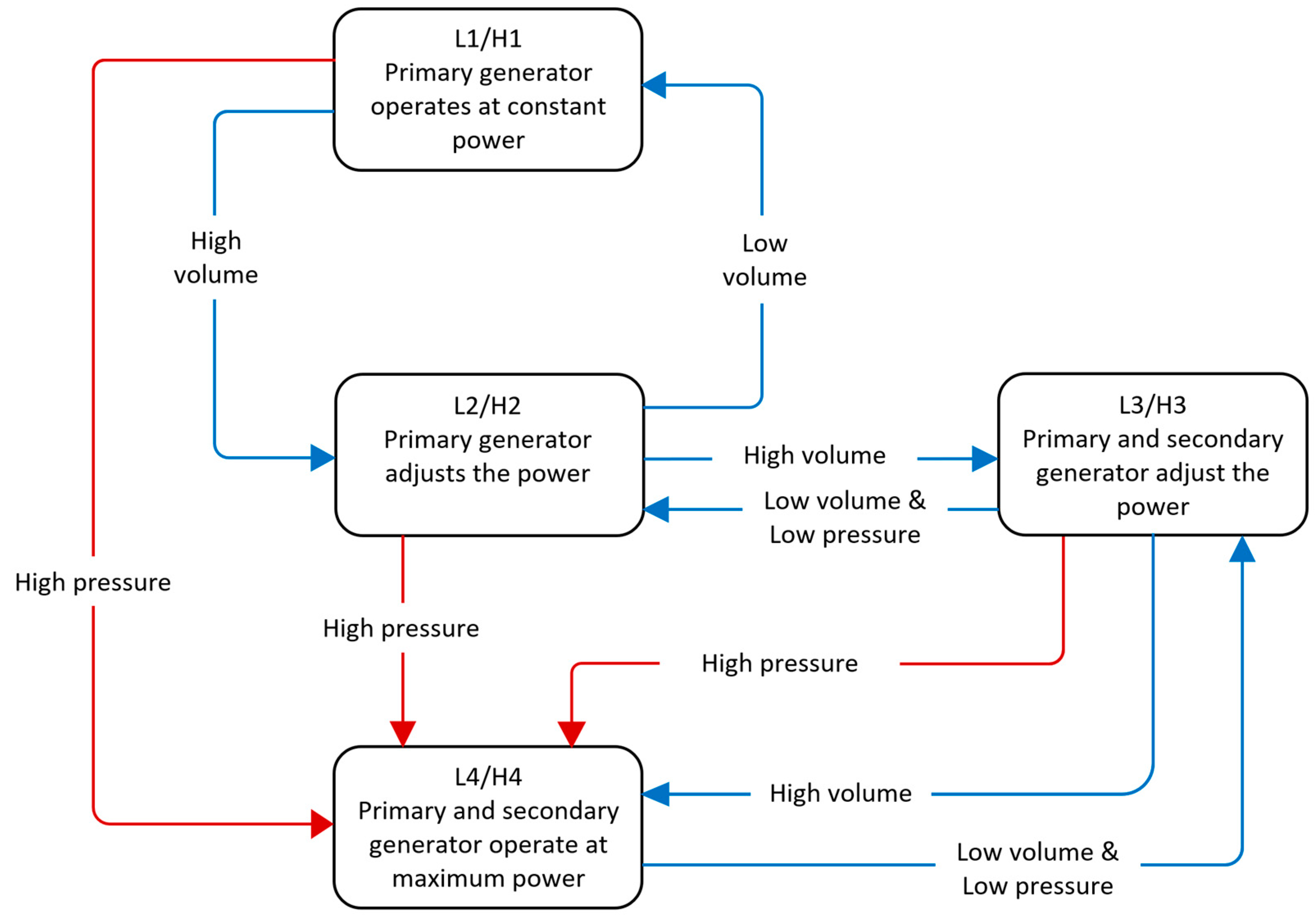
• The primary generator, which operates at the low tariff in state L1, switches to L2 when the volume in the storage tank is greater than 30%.
• From L2, it returns to L1 when the volume falls below 10%, or it switches from L2 to L3 when the volume rises above 85%.
• From L3, it returns to L2 when the volume falls below 15%, and the pressure in the storage tank falls below 0.8 mbar for 15 min.
• Similar conditions also apply for L4 and for operation in high tariffs. The transitions marked in red in Figure 6 apply from any state to L4 (or H4) when the pressure rises above 2.5 mbar for 2 min.

Note that in Table 2, higher volume values have been set for the low tariff transitions (i.e., L1 to L2 and L2 to L3) than for the high tariff transitions (i.e., H1 to H2 and H2 to H3). As a result, less electricity is generated at a low tariff, and gas is saved for electricity generation at a high tariff. To avoid frequent on and off switching of the generators, a time delay (15 min) for the transition to a new state was selected from the various options listed in Section 2.3.1. In modes 2 and 3, the factor $k_E$ is used as described in Section 2.3.2 to adjust the power generation for the low and high tariffs according to (9). The parameters were calibrated during the trial operation and are seldom modified. The most frequently adjusted parameter in daily operation is the factor $k_E$.

3. Results

The results of the proposed control system were evaluated by comparing the operation of the generators and the energy consumption and production during initial operation and operation with dynamic control of biogas engines.

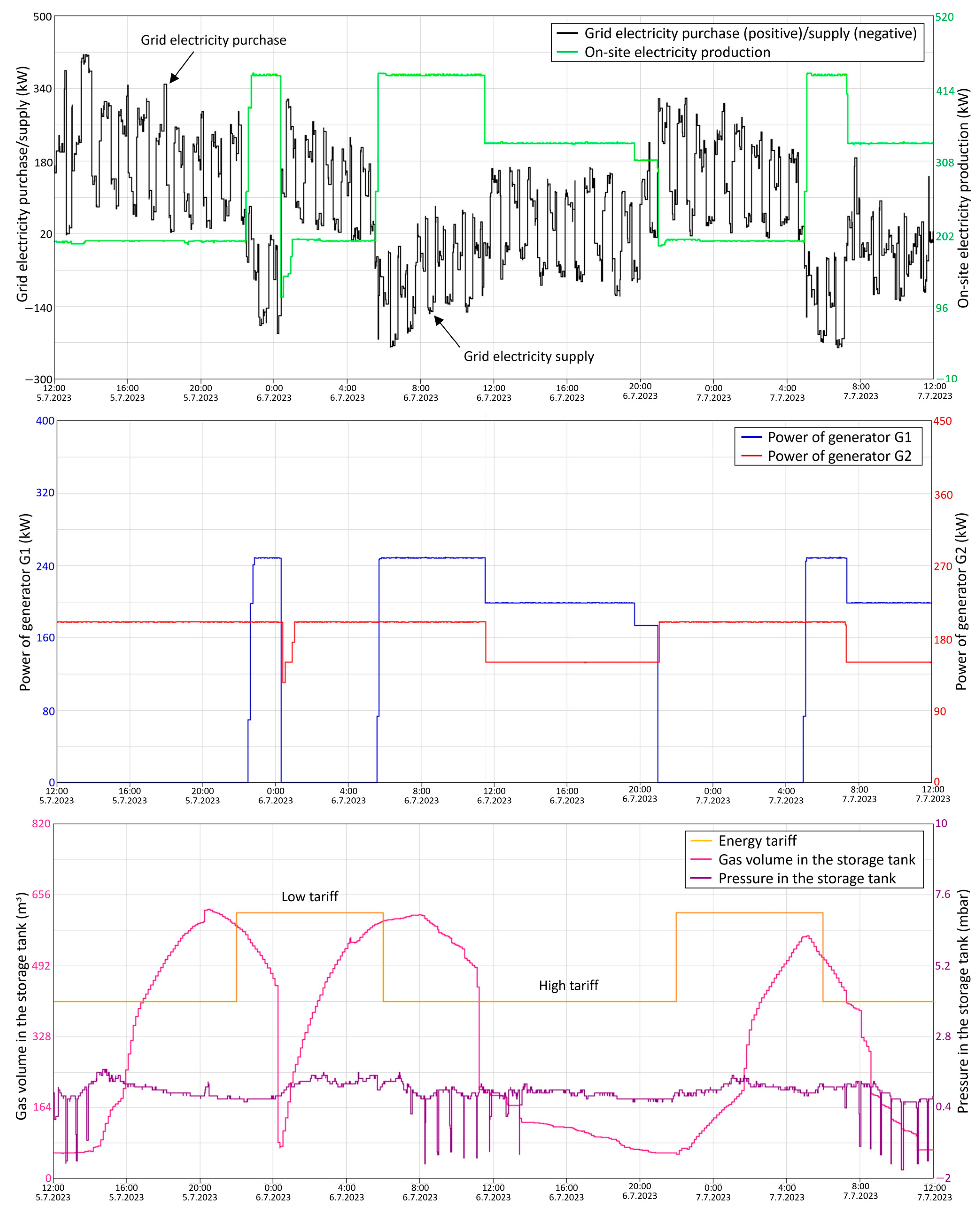
3.1. Initial Operation

In the initial operation, the biogas engines were operated manually, with the operators switching them on and off. In the afternoon and at night, this task was carried out by the staff on duty. This manual approach was prone to human error and challenging to operate 24 h a day. Common operational deficiencies included sub-optimal switching on and off of the generators, inappropriate and inaccurate power adjustments and excessive biogas storage resulting in biogas flaring or insufficient biogas storage resulting in increased dependence on grid electricity. In addition, tracking operating hours and ensuring even utilisation of the two biogas engines proved difficult.

Figure 7 shows an example of the initial operation of the electricity generators for two days. The top diagram shows the purchase and supply of grid electricity, indicated by positive and negative values of grid electricity. Most of the time, additional electricity was purchased from the grid since the electricity generated on-site by switching the generators on and off was insufficient, except for short periods when it exceeded demand. The middle diagram illustrates that the power of generators was only adjusted slightly in rare cases during operation. Switching the generators on and off was not optimal in relation to the gas volume in the storage tank, as can be seen in the bottom diagram. In addition, the measurements of the biogas volume were not entirely reliable, as evidenced by a sudden drop or increase in the biogas volume when the membrane cover of the storage tank was bent.

In many cases during the initial operation, biogas was consumed heavily at the beginning of the high tariff by running both generators at maximum power. Once the biogas storage tank ran out of biogas, one generator was switched off. However, the remaining generator alone did not supply enough electricity to cover the process requirements. Therefore, grid electricity was purchased, which led to higher electricity costs.

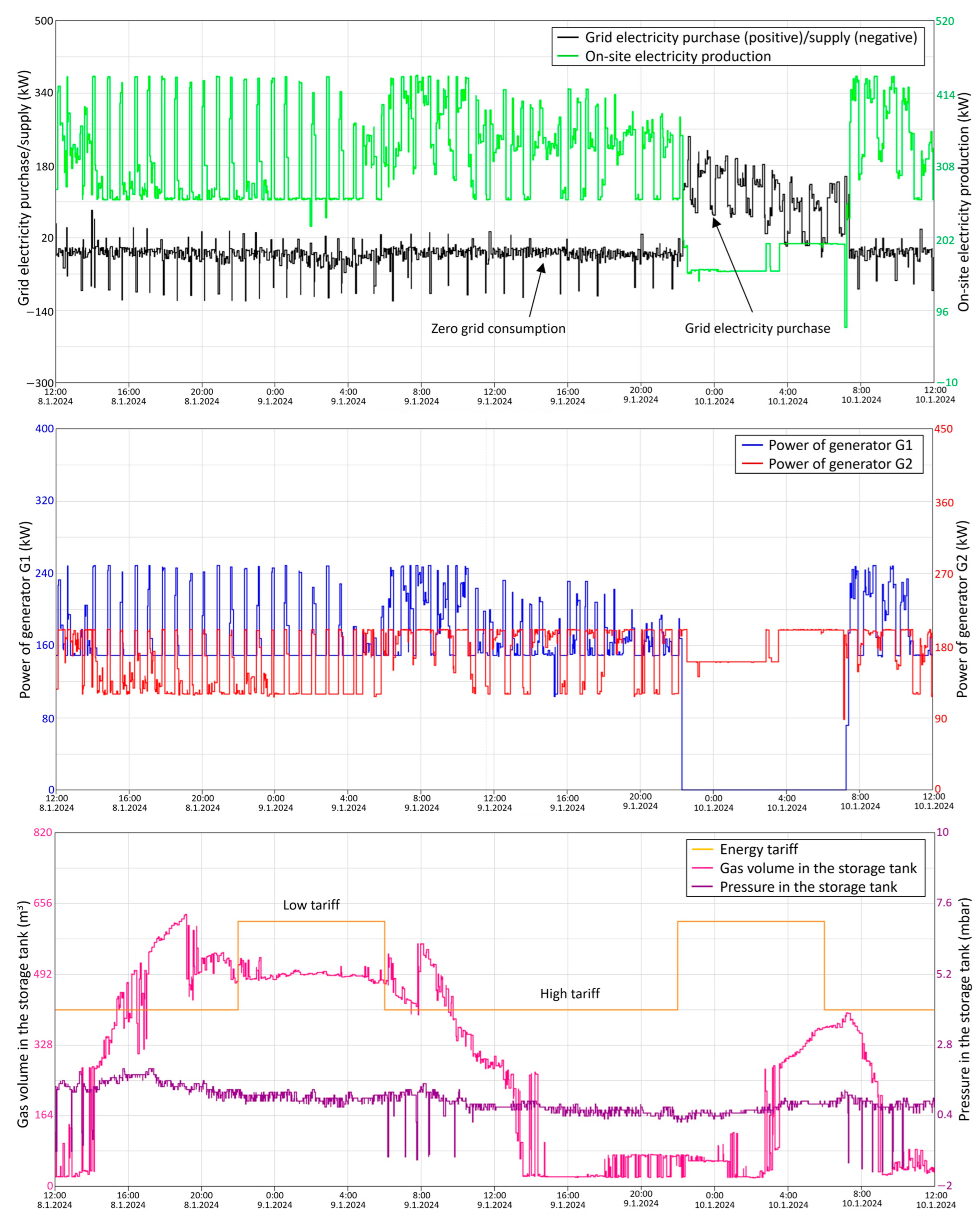
3.2. Operation After Implementation of the Dynamic Control

Figure 8 shows the operation of the electricity generators after the implementation of the proposed dynamic control. The same diagrams as in Figure 7 are shown for two days of operation.

The two upper diagrams show a clear difference compared to Figure 7. The signal representing the electricity purchased or supplied to the grid is close to zero most of the time, which means that the adjustment of electricity generation to the current demand of the technological processes is very efficient. In contrast to Figure 7, electricity generated on site fluctuates strongly and adapts dynamically to the WWTP electricity demand. It can be seen that the WWTP electricity consumption is changing considerably. The highest fluctuations are caused by switching the blowers on and off.

With a moderate level of biogas in the storage tank at a high tariff (lower diagram), both generators operate and dynamically adjust the power to the WWTP demand (middle diagram). If the biogas reserves are not sufficient to operate both generators, the secondary generator switches off at a low tariff (in this case G1). When the biogas volume in the storage tank is higher, the secondary generator switches on again at a high tariff. This enables operation at a high tariff with virtually no power consumption from the grid. Electricity is drawn from the grid almost exclusively during the low tariff, which results in low electricity costs. Figure 8 also shows that the measurements of the biogas volume are more stable due to the implementation of additional sensors at various points and the averaging of the measured values.

3.3. Impact of the Proposed Control

A comparison of electricity generation and consumption at the Domžale-Kamnik WWTP before and after the implementation of the proposed dynamic control algorithm is shown in

Table 3. Comparison of electricity production, consumption and grid supply/off-take before and after implementation of the proposed control.

Electricity Production and Consumption	Unit	Initial Operation January–June 2023	Implemented Dynamic Control January–June 2024
Total on-site electricity generation in biogas engines	kWh	1,612,127	1,493,880
Total electricity consumption at WWTP	kWh	1,482,643	1,391,122
Electricity supply to the grid (sell)	kWh	309,203	200,949
Electricity off-take from the grid (purchase)	kWh	128,935	46,089
Share of consumed electricity purchased from the grid	%	8.7	3.3

. Electricity off-take from the grid was significantly lower after the introduction of automatic control of the biogas engines. It fell from 128,935 kWh in the first six months of 2023 to 46,089 kWh in the same period of 2024, i.e., from 8.7% to 3.3% of the wastewater treatment plant’s total electricity consumption.

The electricity supplied to the grid was also reduced due to the tighter demand-responsive management of self-generated electricity. Overall, this leads to more optimal costs, as selling surplus electricity to the grid at the expense of purchasing electricity to cover the electricity shortfall is not ideal under the energy prices in Table 1. In 2024, electricity production and consumption were lower than in 2023 due to the variations in the input wastewater and anaerobic digestion substrate, which were more diluted in 2024 due to rainfall events.

The techno-economic analysis provided in Supplementary Material S2 shows that the implementation of dynamic control reduces the electricity costs per kWh consumed by 4.1% from € 0.05633/kWh to € 0.05402/kWh. With an electricity consumption of around 2,873,765 kWh/year, this corresponds to an estimated annual cost reduction of €6638. The calculated payback period for implementing this system is less than two years.

4. Discussion

Dynamic control of biogas engines leads to improved performance but also has some limitations. This approach utilises the part-load operation for CHP units. Studies on the environmental impact of flexible power generation in CHP biogas plants show that part- load operation leads to higher greenhouse gas emissions due to lower electrical efficiency under part-load conditions [22]. In addition, the emission values increase during the start-up of CHP systems. Consequently, minimising the number of starts and stops is preferable [17]. In this context, part-load operation offers a potential advantage as it eliminates the need for starting procedures and enables a faster increase rate than starting from the “off” state.

To analyse these issues, the specific electricity production per biogas consumed and the electrical efficiency of the biogas engines were analysed. During the initial operation, the specific electricity production was 2.26 kWh/m³ of biogas, and it decreased slightly to 2.25 kWh/m³ of biogas under dynamic control in 2024. Similarly, the electrical efficiency of the biogas engines decreased from 37.87% to 37.70%. This evaluation suggests that flexible power generation has minimal impact on overall electrical efficiency compared to initial operation. These minor differences may be due to the fact that the engines did not operate consistently at full power even during initial operation (see middle diagram in Figure 7). In addition, the dynamic algorithm linearly increases the power of both engines to avoid operating at minimum power (see upper diagrams in Figure 4). The electrical efficiency has remained high and is close to the typical value of 40% for electricity generation [23]. In addition, the number of start-ups and shutdowns has not changed significantly, as shown in the middle diagrams in Figure 7 and Figure 8.

The dynamic control system only takes the electricity demand into account. The demand for heat generation is not taken into account in the upper-level control system when determining the desired total power of the generators. The reason for this is that heat production currently exceeds the demand of the WWTP. The heat generated is primarily used to heat the anaerobic digesters and to heat the buildings in winter. In summer, the excess heat is released into the air via an external air cooler. In the future, the WWTP is planning to introduce a sludge drying unit to fully utilise the heat generated. If both electricity and heat generation are to be considered, hybrid operation strategies can be used, e.g., master electric tracking slave thermal tracking [21]. Alternatively, optimisation can be used to optimise the thermal-electrical load balancing between the units and find the most economical operating strategy [24].

5. Conclusions

This paper proposes an energy cost optimisation strategy that adjusts the power of CHP units in a WWTP to reduce grid electricity costs. This is achieved by dynamic control of on-site electricity generation subject to different criteria (e.g., the amount of self-generated electricity, the energy demand of the WWTP, energy tariffs, gas storage reserves, etc.). The proposed control algorithm is designed as a two-level control system, where the upper-level control takes into account the optimisation requirements by appropriately determining the total power set-point, while the lower control level adjusts the power of the individual units in a unique way and regardless of the optimisation requirements.

The algorithm was implemented at a full-scale WWTP, resulting in a reduction in the grid electricity consumption from 8.7% to 3.3% of the WWTP’s total electricity demand. This reduction was achieved through the optimisation and dynamic control of biogas engines. Because of the different prices for the grid electricity and the on-site generated electricity in CHP units, the reduced grid electricity consumption resulted in a 4.1% reduction in total electricity costs.

In this case, demand-driven electricity generation was implemented at the WWTP level to adapt electricity generation to the WWTP demand. In the future, it can be integrated into demand-driven dispatchable electricity generation to adapt electricity generation to short-term grid electricity demand if attractive cost models for grid electricity supply are offered.

References

1. Campana, P.E.; Mainardis, M.; Moretti, A.; Cottes, M. 100% renewable wastewater treatment plants: Techno-economic assessment using a modelling and optimization approach. Energy Convers. Manag. 2021, 239, 114214. [Google Scholar] [CrossRef]
2. Riley, D.M.; Tian, J.; Güngör-Demirci, G.; Phelan, P.; Villalobos, J.R.; Milcarek, R.J. Techno-Economic Assessment of CHP Systems in Wastewater Treatment Plants. Environments 2020, 7, 74. [Google Scholar] [CrossRef]
3. Tsalas, N.; Golfinopoulos, S.K.; Samios, S.; Katsouras, G.; Peroulis, K. Optimization of Energy Consumption in a Wastewater Treatment Plant: An Overview. Energies 2024, 17, 2808. [Google Scholar] [CrossRef]
4. Maktabifard, M.; Zaborowska, E.; Makinia, J. Achieving energy neutrality in wastewater treatment plants through energy savings and enhancing renewable energy production. Rev. Environ. Sci. Biotechnol. 2018, 17, 655–689. [Google Scholar] [CrossRef]
5. Åmand, L.; Olsson, G.; Carlsson, B. Aeration control—A review. Water Sci. Technol. 2013, 67, 2374–2398. [Google Scholar] [CrossRef]
6. Gu, Y.; Li, Y.; Yuan, F.; Yang, Q. Optimization and control strategies of aeration in WWTPs: A review. J. Clean. Prod. 2023, 418, 138008. [Google Scholar] [CrossRef]
7. Monday, C.; Zaghloul, M.S.; Krishnamurthy, D.; Achari, G.A. Review of AI-Driven Control Strategies in the Activated Sludge Process with Emphasis on Aeration Control. Water 2024, 16, 305. [Google Scholar] [CrossRef]
8. Brok, N.B.; Munk-Nielsen, T.; Madsen, H.; Stentoft, P.A. Unlocking energy flexibility of municipal wastewater aeration using predictive control to exploit price differences in power markets. Appl. Energy 2020, 280, 115965. [Google Scholar] [CrossRef]
9. Liu, Q.; Dereli, R.K.; Flynn, D.; Casey, E. Demand response through reject water scheduling in water resource recovery facilities: A demonstration with BSM2. Water Res. 2021, 188, 116516. [Google Scholar] [CrossRef]
10. Aymerich, I.; Rieger, L.; Sobhani, R.; Rosso, D.; Corominas, L. The difference between energy consumption and energy cost: Modelling energy tariff structures for water resource recovery facilities. Water Res. 2015, 81, 113–123. [Google Scholar] [CrossRef]
11. Firouzian, M.; Stenstrom, M.K.; Rosso, D. Effects of power tariffs and aeration dynamics on the expansion of water resource recovery facilities. J. Clean. Prod. 2022, 337, 130385. [Google Scholar] [CrossRef]
12. Ali, S.M.H.; Lenzen, M.; Sack, F.; Yousefzadeh, M. Electricity generation and demand flexibility in wastewater treatment plants: Benefits for 100% renewable electricity grids. Appl. Energy 2020, 268, 114960. [Google Scholar] [CrossRef]
13. Liu, Q.; Li, R.; Dereli, R.K.; Flynn, D.; Casey, E. Water resource recovery facilities as potential energy generation units and their dynamic economic dispatch. Appl. Energy 2022, 318, 119199. [Google Scholar] [CrossRef]
14. Kirchem, D.; Dereli, R.K.; Lynch, M.Á.; Casey, E. Demand response within the Irish wastewater treatment sector: Analysing flexibility potentials of the aeration process and wastewater pumping within an integrated energy–water system model. Appl. Energy 2025, 381, 125128. [Google Scholar] [CrossRef]
15. Lafratta, M.; Thorpe, R.B.; Ouki, S.K.; Shana, A.; Germain, E.; Willcocks, M.; Lee, J. Dynamic biogas production from anaerobic digestion of sewage sludge for on-demand electricity generation. Bioresour. Technol. 2020, 310, 123415. [Google Scholar] [CrossRef] [PubMed]
16. Hochloff, P.; Braun, M. Optimizing biogas plants with excess power unit and storage capacity in electricity and control reserve markets. Biomass Bioenergy 2014, 65, 125–135. [Google Scholar] [CrossRef]
17. Ishikawa, S.; Connell, N.O.; Lechner, R.; Hara, R.; Kita, H.; Brautsch, M. Load response of biogas CHP systems in a power grid. Renew. Energy 2021, 170, 12–26. [Google Scholar] [CrossRef]
18. Schäfer, M. Short-term flexibility for energy grids provided by wastewater treatment plants with anaerobic sludge digestion. Water Sci. Technol. 2020, 81, 1388–1397. [Google Scholar] [CrossRef]
19. Musabandesu, E.; Loge, F. Load shifting at wastewater treatment plants: A case study for participating as an energy demand resource. J. Clean. Prod. 2021, 282, 124454. [Google Scholar] [CrossRef]
20. Chapin, F.T.; Bolorinos, J.; Mauter, M.S. Electricity and natural gas tariffs at United States wastewater treatment plants. Sci. Data 2024, 11, 113. [Google Scholar] [CrossRef]
21. Cappiello, F.L.; Erhart, T.G. Modular cogeneration for hospitals: A novel control strategy and optimal design. Energy Convers. Manag. 2021, 237, 114131. [Google Scholar] [CrossRef]
22. Hijazi, O.; Tappen, S.; Effenberger, M. Environmental impacts concerning flexible power generation in a biogas production. Carbon Resour. Convers. 2019, 2, 117–125. [Google Scholar] [CrossRef]
23. Longo, S.; Mauricio-Iglesias, M.; Soares, A.; Campo, P.; Fatone, F.; Eusebi, A.L.; Akkersdijk, E.; Stefani, L.; Hospido, A. ENERWATER—A standard method for assessing and improving the energy efficiency of wastewater treatment plants. Appl. Energy 2019, 242, 897–910. [Google Scholar] [CrossRef]
24. Wang, Z.; Gu, Y.; Liu, H.; Li, C. Optimizing thermal–electric load distribution of large-scale combined heat and power plants based on characteristic day. Energy Convers. Manag. 2021, 248, 114792. [Google Scholar] [CrossRef]
Figure 1. Cogeneration of renewable electricity and heat from biogas obtained in anaerobic digestion.
Water 17 01170 g001
Figure 2. Control scheme for power management of CHP generators.
Water 17 01170 g002
Figure 3. Relation between minimum power of generators G1 and G2 to achieve ideal total power characteristic curve in case of P 1 m a x = 300  kW, P 2 m a x = 210 kW and selected hysteresis H.
Water 17 01170 g003
Figure 4. Distribution of power between generators G1 and G2 and the total power in the case of primary generator G1 (left) and primary generator G2 (right). The blue lines represent the situation when the total power increases and the red dotted lines represent the situation when the total power decreases. The green dashed line represents the ideal case. The generator characteristics are as follows: P 1 m i n = 150   kW, P 1 m a x = 300   kW, P 2 m i n = 120   kW, P 2 m a x = 210   kW, and H = 30   kW.
Water 17 01170 g004
Figure 5. Volume in the gas storage tank with indicated normal operating range between V L  and V H .
Water 17 01170 g005
Figure 6. Diagram of the state machines used in the low tariff (states L1, L2, L3, L4) and high tariff (states H1, H2, H3 and H4). The transitions between the states are determined on the basis of the gas volume and pressure conditions in the gas storage tank. They can be set differently for each state machine.
Water 17 01170 g006
Figure 7. Initial operation of electricity generators: grid electricity purchase/supply and on-site electricity production (top); power of generators G1 and G2 (middle); energy tariff, volume and pressure in the gas storage tank (bottom).
Water 17 01170 g007
Figure 8. Operation of electricity generators after implementation of the dynamic control of generators: grid electricity purchase/supply and on-site electricity production (top); power of generators G1 and G2 (middle); energy tariff, volume and pressure in the gas storage tank (bottom).
Water 17 01170 g008