Adaptive Penetration Unit for Deep-Sea Sediment Cone Penetration Testing Rigs: Dynamic Modeling and Case Study

Abstract

The reliability and continuity of data are key issues in deep-sea sediment cone penetration testing. Cone penetration testing employs static force to uniformly insert rods into sediment, a process crucial for assessing its mechanics and layering. The clamping manipulator can perform this operation while accommodating sediment sensors of varying types and sizes. However, its requirement to reset post-penetration creates zero-velocity points that diminish test continuity and should be minimized. To address these limitations, this paper proposes a load-adaptive sediment rig that minimizes zero-velocity points, ensures data continuity, and contributes to sedimentology research. This paper analyzes the mechanical properties and layering patterns of sediment, along with the interaction mechanisms between sediment and mechanical structures. Subsequently, a mechanical structure–sediment-integrated model with adaptive control logic is established. Finally, real sediment data are introduced into the physical model for simulation experiments. The simulation results demonstrate that the load-adaptive rig reduces data breakpoints by 50% and increases the maximum single penetration stroke to 1.8 m. Additionally, the load-adaptive rig provides redundancy between penetration force and stroke, automatically reducing penetration force for greater stroke when encountering low-strength sediments and, conversely, sacrificing part of the stroke for greater force. These improvements significantly enhance the continuity of in situ detection data of sediment.

1. Introduction

Cone penetration testing (hereinafter referred to as CPT) is the most commonly used in situ testing method for the mechanical properties of seabed sediments [1]. By pressing the cone rod with specific sensors into the sediment at a constant penetration rate, parameters such as cone resistance, sleeve friction, and pore water pressure are measured, and the relationship between the CPT data and the sediment mechanical parameters is established by a semi-theoretical and semi-empirical method, so as to indirectly obtain the physical and mechanical properties of the sediment layer [2,3,4]. With the continuous development of sensor technology, the CPT technique can provide more reliable and multi-parameter test data by replacing and developing different probes and sensors, so this in situ testing method has great expandability [5].

Cone penetration testing has been applied to sediment testing since the 1960s [6]. Due to its characteristics of its real-time, efficient, and accurate determination of the engineering properties of submarine soils, it has unparalleled advantages in the comprehensive evaluation of submarine engineering geology [7,8]. Some countries regard cone penetration technology as an essential part of marine engineering geological surveys, and it has been applied in the following areas: (1) To identify sediment types, delineate strata, and determine the vertical stratification of sediment conditions; (2) To estimate the physical and mechanical properties of soil to reflect the engineering properties of subsea soil, such as estimating soil shear strength and the overconsolidation ratio; (3) Piezocone penetration tests (CPTUs), building on traditional CPT, can measure pore water pressure, providing a more accurate reflection of soil liquefaction trends and electrical resistivity [9,10,11]. A number of reliable commercial seabed-based CPT rigs are now available on the market, such as the ROSON series, the Neptune series, the Manta series, and the Seacalf series [12,13,14]. These CPT rigs can operate in water depths of up to 3000 meters and are powered by electrical energy transmitted from surface vessels via umbilical cables [15]. Depending on the penetration method, these devices can be divided into two categories: friction wheel and manipulator [16,17]. One of the most important features of this equipment, represented by the Neptune 3000, is the use of pairs of rolling metal wheels to extrude and straighten flexible rods, using friction to achieve penetration of the rods [18,19]. Another common type of rig uses a clamping manipulator for the penetration of the rod [20,21]. During the penetration operation, the upper movable clamping manipulator is in a clamped state, while the lower fixed manipulator is in a released state [22,23]. At this time, the driving hydraulic cylinder piston rod extends, transmitting through the steel cable and pulley block, which drives the movable manipulator on the sliding seat to clamp the rod and slowly and uniformly penetrate into the soil. After a single penetration is completed, the lower fixed manipulator clamps the rod, the upper movable one releases, the penetration cylinder piston rod retracts, and the upper movable manipulator resets. This is one penetration cycle [24]. Repeating the above cycle completes the full penetration of the rod.

The penetration of the rod is subjected to continuous resistance exerted by the soil layer, which usually fluctuates dramatically due to the complexity of the formation [25,26]. In order to collect high-quality raw data in this case, it is required that the penetration speed of the rod with the sensor is kept constant during the test, e.g., 2 cm/s [27,28,29]. The above-mentioned Neptune 3000 can easily achieve continuous penetration of tens of meters in a single operation due to the use of flexible rods that can be coiled and stowed as well as the metal wheel penetration device. However, due to the poor adaptability of the metal wheels to the diameter of the rods, the cross-sectional area of the tens of meters of the rods of the Neptune 3000 is kept to 2.5 ${\mathrm{cm}}^2$, which means that the types of sensors that can be accommodated in such a small space are very limited [30,31]. Therefore, the disadvantages of this type of CPT rig are the small variety of parameters acquired and the weak representativeness of the data. Another type of rig uses a clamping manipulator to achieve the penetration of the rod. Although the flexible opening and closing range of its manipulator can accommodate rods of different diameters, after completing a single penetration, the manipulator needs to release its clamp and reset to proceed to the next penetration cycle. During the resetting process, the speed of the rod is 0, so the working continuity of such equipment is relatively poor. In addition, the maximum penetration force and the depth of a single penetration of this equipment are fixed. When encountering soil layers with low resistance (low-load conditions), it is difficult to fully utilize the rig.

Based on the analysis above, to address the problems of clamping manipulators, this paper proposes a load-adaptive CPT rig with the aim of achieving gear shifting according to dynamic loads and obtaining the maximum single penetration stroke under load conditions based on the clamping manipulator-type CPT. The rig uses a pulley assembly to multiply the displacement of the driving hydraulic cylinder, and the pulleys that make up this assembly can switch between fixed pulley and movable pulley states. Therefore, by changing the number of enabled movable pulleys in the pulley assembly, the amplification factor of the hydraulic cylinder displacement can be altered, which, in turn, changes the single penetration stroke of the clamping manipulator. This process is defined as gear shifting in this paper.

The main novelties of this paper are as follows: We propose a load-adaptive CPT rig with a variable pulley block, enhancing stroke under load, minimizing rate zeros, and ensuring data continuity. This paper establishes a mathematical model of the hydraulic cylinder, analyzes its amplitude–frequency characteristics, determines the boundary conditions, and verifies the model through physical simulation. We validate the model using real CPT data, demonstrating the load-adaptive CPT system’s superior continuity and efficiency under identical resistance conditions compared to conventional systems. In strata with low resistance, the system automatically shifts to a higher gear, applying minimal yet sufficient force for maximum penetration, which ensures data reliability and continuity while optimizing energy efficiency through force conservation.

The paper is organized as follows: Section 2 introduces the structural design of the load-adaptive CPT rig and the shifting method of the penetration unit; Section 3 details the development and subsequent validation of the system’s mathematical model; and Section 4 tests the CPT rig utilizing actual CPT data and, subsequently, analyzes the resulting test outcomes.

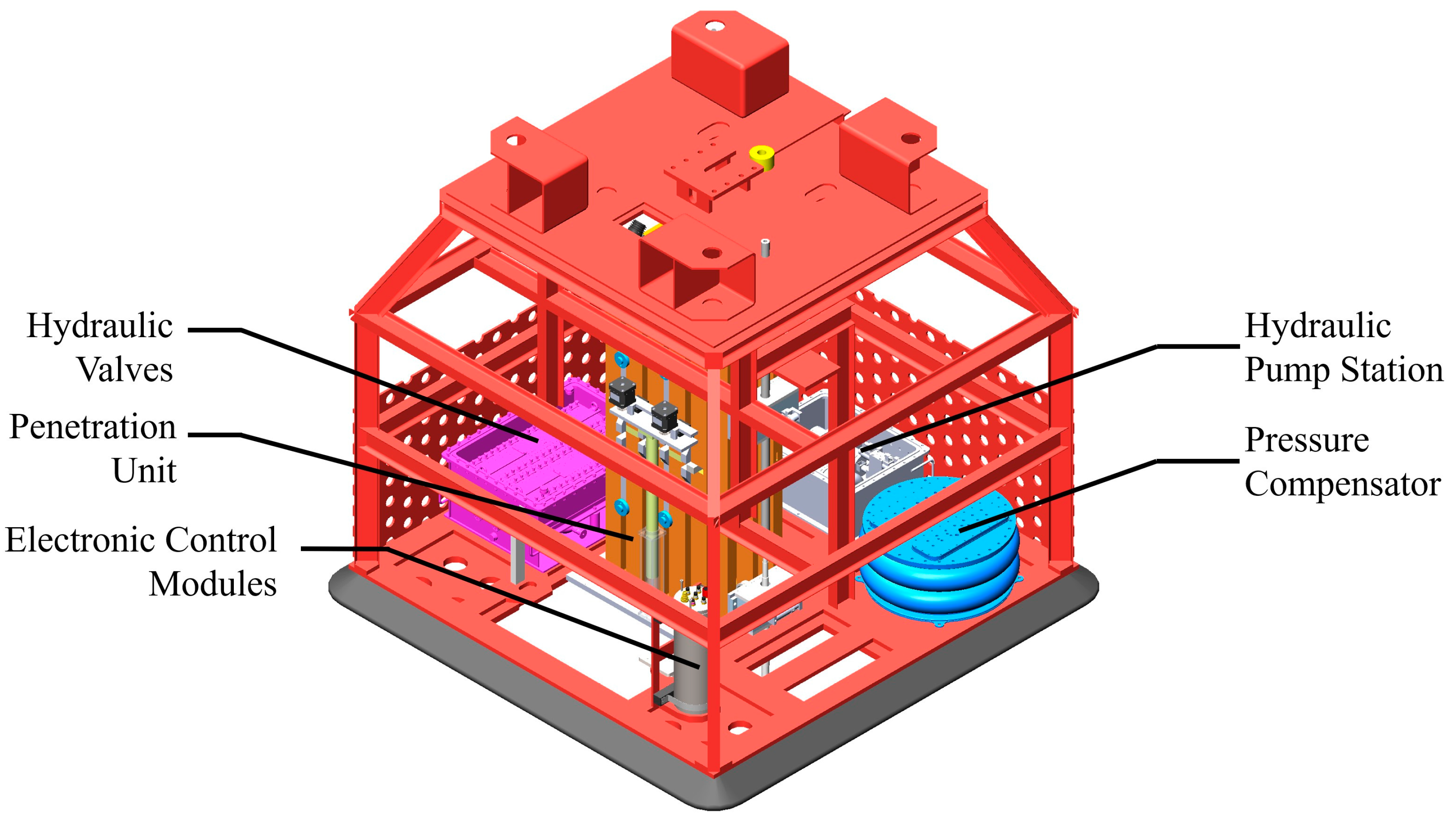
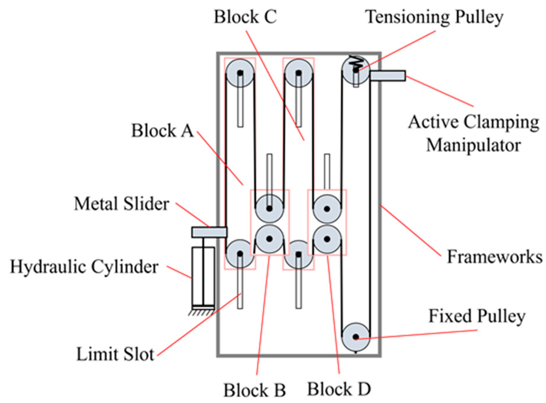
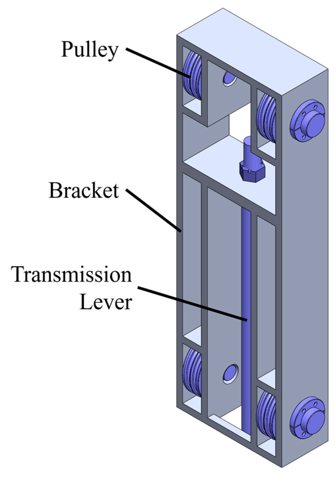
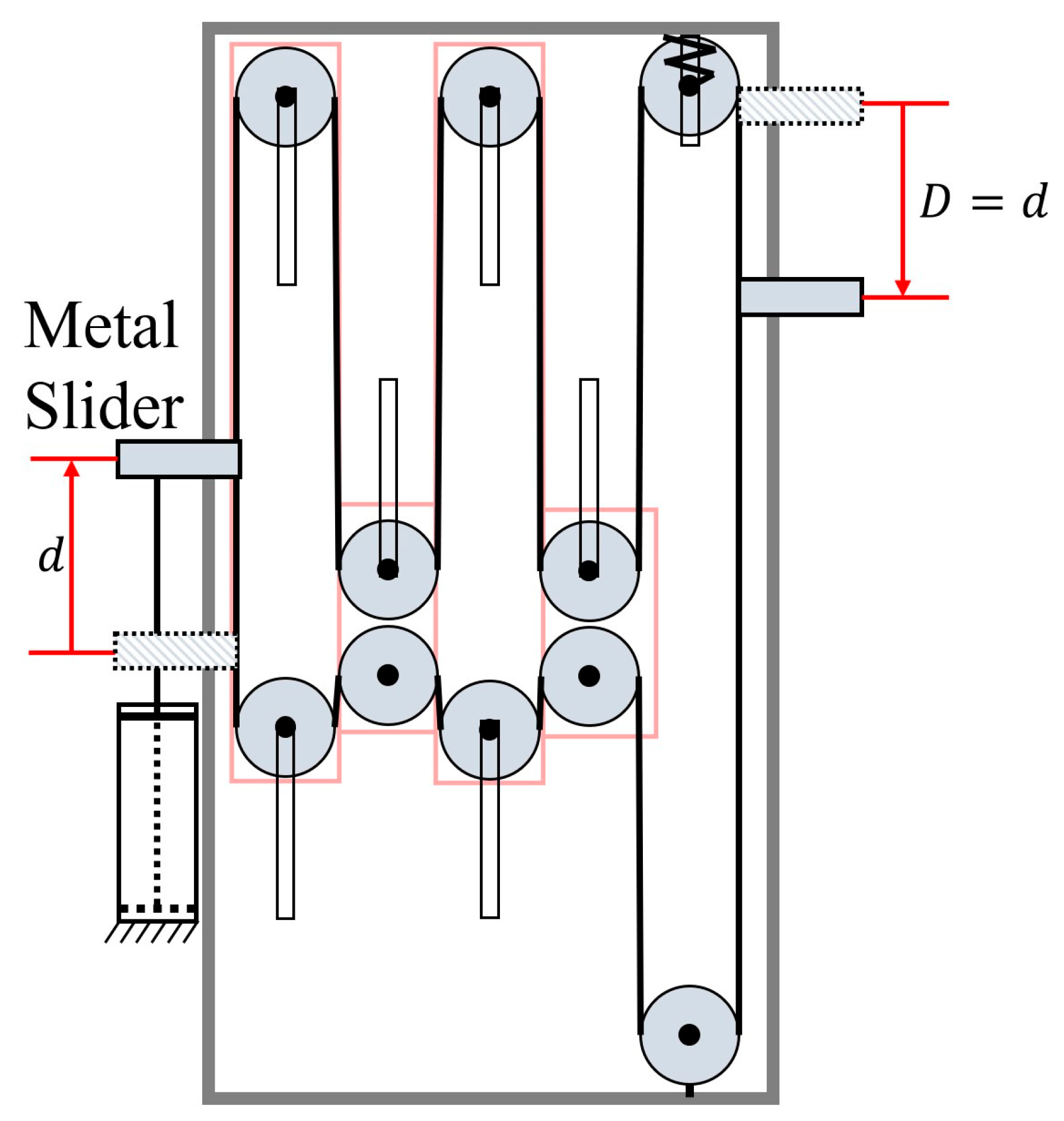
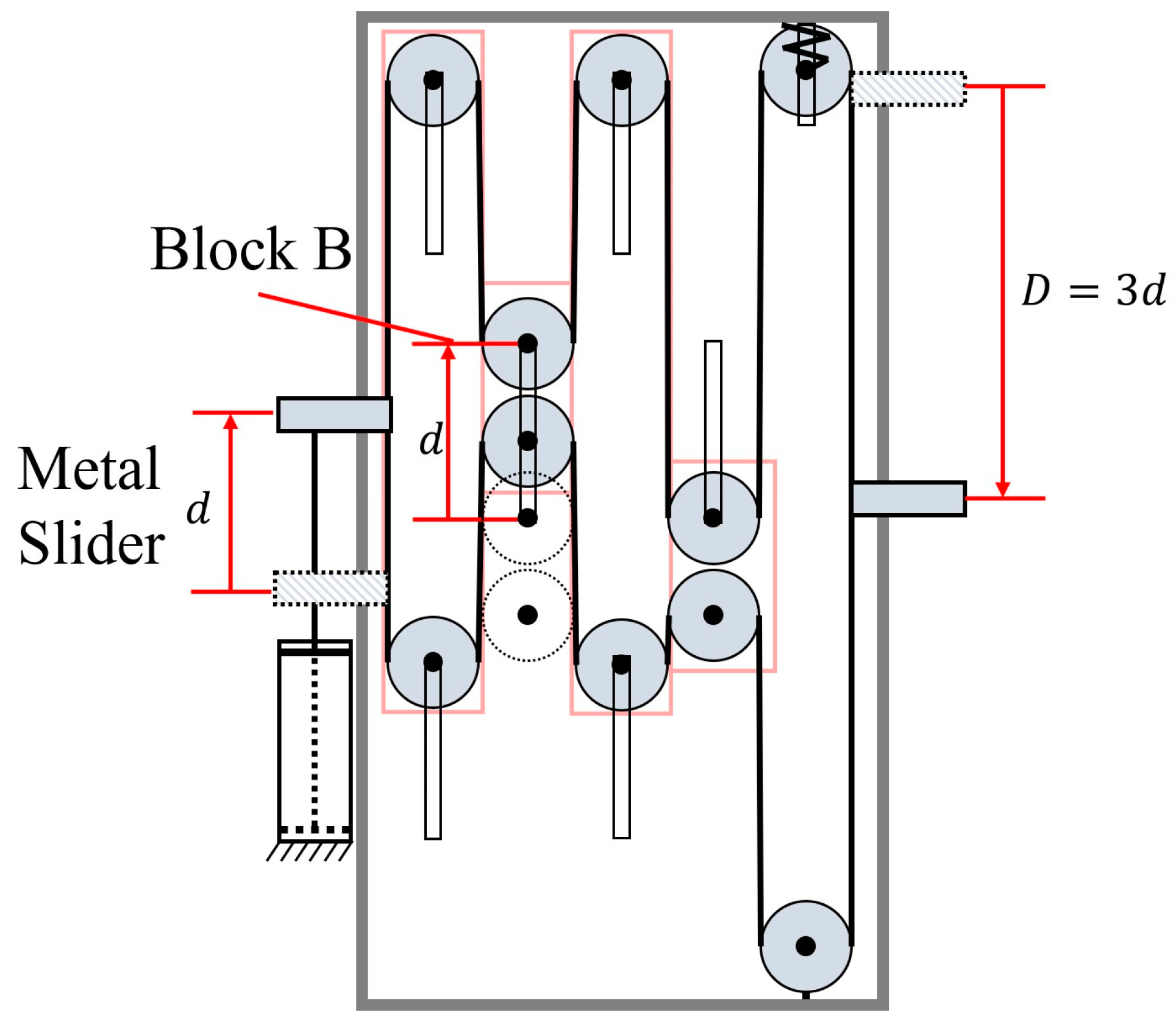
2. Structure of the Load-Adaptive CPT Rig

Figure 1 describes the general structure of the load-adaptive CPT rig, and Figure 2 shows the specific structure of the penetration unit. During the penetration test, the active clamping manipulator is in the clamping state, and the lower fixed clamping manipulator is in the loosening state; at this time, the piston rod of the hydraulic cylinder extends and drives the active clamping manipulator to clamp the rod slowly and evenly into the soil layer by means of the transmission of the steel cable and pulley group. After the single penetration is completed, the lower fixed clamping manipulator clamps the rod, the upper movable clamping manipulator is loosened, the piston rod of the penetration cylinder is retracted, the upper movable clamping manipulator is reset, and the above cycle is repeated until the rod penetrates to the specified depth.

Figure 2 and Figure 3 depict the structure and operational mechanism of the penetration unit. The unit’s central components are the pulley block and steel cable. Within the unit, pulleys are categorized into two types: central pulleys and distal pulleys. For instance, Blocks B and D in Figure 3 are central pulleys, while Blocks A and C are distal pulleys. As observed in Figure 4, the pulleys are mounted on a bracket to constitute a pulley block, ensuring synchronized velocity among pulleys within the same block. Furthermore, the steel cable’s end is secured to a metal slider, enabling the cable to move in unison with the slider’s motion. The pulley and metal slider are both connected to the hydraulic cylinder via a clutch, remaining stationary when the clutch is disengaged. Upon the pin clutch’s activation, pushing the pin into the designated groove, the central pulley and metal slider are actuated by the hydraulic cylinder, initiating movement. Concurrently, the central pulley propels the sprocket chain assembly into motion; as the chain clutch secures the chain, the distal pulley synchronizes with the chain, moving in unison. These clutch mechanisms enable the control and switching of the pulley between two states in both fixed and dynamic pulleys.

When the hydraulic cylinder directly actuates the metal slider, the cylinder’s stroke is transferred to the clamping manipulator at a 1:1 ratio. According to the principle of the dynamic pulley, the stroke is doubled for each dynamic pulley engaged by the hydraulic cylinder. By altering the number of enabled dynamic pulleys, we can adjust the stroke amplification of the hydraulic cylinder, effectively shifting gears. As depicted in Figure 5, during the transition to the first gear, the driving hydraulic cylinder propels the metal slider upward, with the slider’s displacement denoted as $d$, propelled by the driving force $F_i$ from the cylinder. The metal slider is concurrently subjected to the vertical upward force $F_i$ and the vertical downward cable tension $T$. Thus, when it undergoes uniform linear motion, the following equation holds:

$$F_i=T$$

(1)

Subsequently, the penetration force output by the system in the first gear is as follows:

$$F_{o1}=T=F_i$$

(2)

Due to the presence of the tensioning wheel, the change in the length of the steel cable is negligible. At this point, the system’s output displacement, which is also the penetration travel, is $D=d$. Differentiating this with respect to time yields the relationship between the hydraulic cylinder piston velocity $v_{i1}$ and the output velocity $v_o$, as follows:

$$v_{i1}=\dot{d}=\dot{D}=v_o$$

(3)

Additionally, to maintain the penetration speed, namely, the output speed, at 2 cm/s, the velocity of the hydraulic cylinder piston in the first gear is:

$$v_{i1}=2\mathrm{cm}/\mathrm{s}$$

(4)

As shown in Figure 6, when shifted to the second gear, the driving hydraulic cylinder propels Block B upward, at which point Block B has a displacement of $d$ and is subjected to the driving force $F_i$ from the hydraulic cylinder. For Block B, it simultaneously experiences the vertical upward driving force $F_i$ and the vertical downward cable tension $T$. According to the principle of the movable pulley, during uniform linear motion, the following equation holds:

$$F_i=2T$$

(5)

$$D=2d$$

(6)

Therefore, the penetration force output by the system in second gear is:

$$F_{o2}=T={{\displaystyle \frac{1}{2}}F}_i$$

(7)

The velocity of the hydraulic cylinder piston is:

$$v_{i2}=\dot{d}={\displaystyle \frac{1}{2}}\dot{D}={\displaystyle \frac{1}{2}}{v}_o=1\mathrm{cm}/\mathrm{s}$$

(8)

As depicted in Figure 7, when shifted to the third gear, the driving hydraulic cylinder simultaneously propels the metal slider and Block B upward. At this juncture, the driving force $F_i$ from the hydraulic cylinder can be divided into two components: the force $F_{\mathit{iS}}$ acting on the metal slider and the force $F_{\mathit{iB}}$ acting on Block B, that is:

$$F_i=F_{\mathit{iS}}+F_{\mathit{iB}}$$

(9)

The force conditions for the metal slider and Block B are consistent with Equations (1) and (5), hence:

$$F_i=F_{\mathit{iS}}+F_{\mathit{iB}}=T+2T=3T$$

(10)

Similarly, the system’s output displacement is:

$$D=d+2d=3d$$

(11)

Thus, in the third gear state, the penetration force and the velocity of the hydraulic cylinder piston are, respectively:

$$F_{o3}=T={ {\displaystyle \frac{1}{3}}F}_i$$

(12)

$$v_{i2}=\dot{d}={\displaystyle \frac{1}{3}}\dot{D}={\displaystyle \frac{1}{3}}{v}_o\approx 0.33\mathrm{cm}/\mathrm{s}$$

(13)

In summary, the motion states and parameters at different gear positions during the penetration process are summarized in

Table 1. Motion states and parameters at different gears.

	Gear I	Gear II	Gear III	Gear IV	Gear V	Gear VI	Gear VII	Gear VIII	Gear IX
Pulley Block A	╳	╳	╳	↓	↓	↓	↓	↓	↓
Pulley Block B	╳	↑	↑	↑	↑	↑	↑	↑	↑
Pulley Block C	╳	╳	╳	╳	╳	╳	╳	↓	↓
Pulley Block D	╳	╳	╳	╳	╳	↑	↑	↑	↑
Stroke Amplification	0	$\times$2	$\times$2	$\times$4	$\times$4	$\times$6	$\times$6	$\times$8	$\times$8
Metal Slider	↑	╳	↑	╳	↑	╳	↑	╳	↑
Total Stroke Amplification	$\times$1	$\times$2	$\times$3	$\times$4	$\times$5	$\times$6	$\times$7	$\times$8	$\times$9
Penetration Force	F	${\displaystyle \frac{1}{2}}$F	${\displaystyle \frac{1}{3}}$F	${\displaystyle \frac{1}{4}}$F	${\displaystyle \frac{1}{5}}$F	${\displaystyle \frac{1}{6}}$F	${\displaystyle \frac{1}{7}}$F	${\displaystyle \frac{1}{8}}$F	${\displaystyle \frac{1}{9}}$F
Hydraulic Cylinder Speed	2 cm/s	1 cm/s	0.67 cm/s	0.5 cm/s	0.4 cm/s	0.33 cm/s	0.29 cm/s	0.25 cm/s	0.22 cm/s
Penetration Speed	2 cm/s

, where “╳” indicates that the slider or pulley is in a fixed state, “↑” or “↓” signifies an active state capable of moving in the direction of the arrow, and “×2”, “×4”, etc., indicates magnification, and “F” is force. It should be noted that as the stroke of the hydraulic cylinder is magnified, the penetration force decreases inversely. Therefore, we need to flexibly shift gears based on the actual penetration resistance to ensure maximum single-penetration travel under load conditions.

3. Modeling of the Hydraulic Drive System for the Penetration Unit

3.1. Modeling of Servo Valve Mechatronics Subsystem

This paper selected the Bosch Rexroth 4WSE2EM6-2X15BET type servo valve, and its parameters are shown in

Table 2. Parameters and values of the servo valve.

Parameters	Symbol (Unit)	Values
Flow-pressure coefficient	$K_c({\mathrm{m}}^5/\mathrm{N}·\mathrm{s})$	$6.11\times {10}^{-12}$
Internal leakage coefficient	$C_{\mathit{ip}}({\mathrm{m}}^5/\mathrm{N}·\mathrm{s})$	$3\times {10}^{-13}$
External leakage coefficient	$C_{\mathit{ep}}({\mathrm{m}}^5/\mathrm{N}·\mathrm{s})$	0
Equivalent leakage coefficient	$C_{\mathit{ie}}({\mathrm{m}}^5/\mathrm{N}·\mathrm{s})$	$3.36\times {10}^{-13}$
Additional leakage coefficient	$C_f({\mathrm{m}}^5/\mathrm{N}·\mathrm{s})$	$-$3.55$\times {10}^{-14}$
Natural frequency	Wh (rad/s)	268
Flow gain	Ksv (m3/s ∙ A)	4.38 $\times {10}^{-4}$
Bandwidth of servo valve	ωsv (rad/s)	0.03
Damping ratio of servo valve	ξsv	0.6

. This section and the following chapters carry out mathematical modeling based on the parameters of this type of servo valve. The mechatronic subsystem of the servo valve is capable of converting an input voltage signal $u$ into a displacement $x_v$ of the servo valve spool. Specifically, the input voltage $u$ is first converted into a current $i$ by a servo amplifier; the current $i$ is then applied to the coil of the torque motor of the mechatronic converter, causing a force to be generated by a permanent magnet, which is ultimately transferred to the servo valve spool through a mechanical feedback and causes it to generate a displacement $x_v$.

The mathematical model of the servo amplifier is shown below:

$$K_0\left(S\right)={\displaystyle \frac{I(S)}{U(S)}}$$

(14)

where $I(S)$ is the output current, $U(S)$ is the input voltage, and $K_0\left(S\right)$ is the gain amplifier.

In engineering applications, it is a common assumption that an electromechanical transducer can be modeled as a second-order system, neglecting the dead zone, and its mathematical representation is shown below 32:

$${\displaystyle \frac{X_v(S)}{I(S)}}={\displaystyle \frac{K_{\mathit{sv}}}{\frac{S^2}{{{\omega }_{\mathit{sv}}}^2}+\frac{{2\xi }_{\mathit{sv}}S}{{\omega }_{\mathit{sv}}}+1}}$$

(15)

where $K_{\mathit{sv}}$ is the flow gain of servo valve, ${\omega }_{\mathit{sv}}$ is the bandwidth of servo valve, and ${\xi }_{\mathit{sv}}$ is the damping ratio of servo valve.

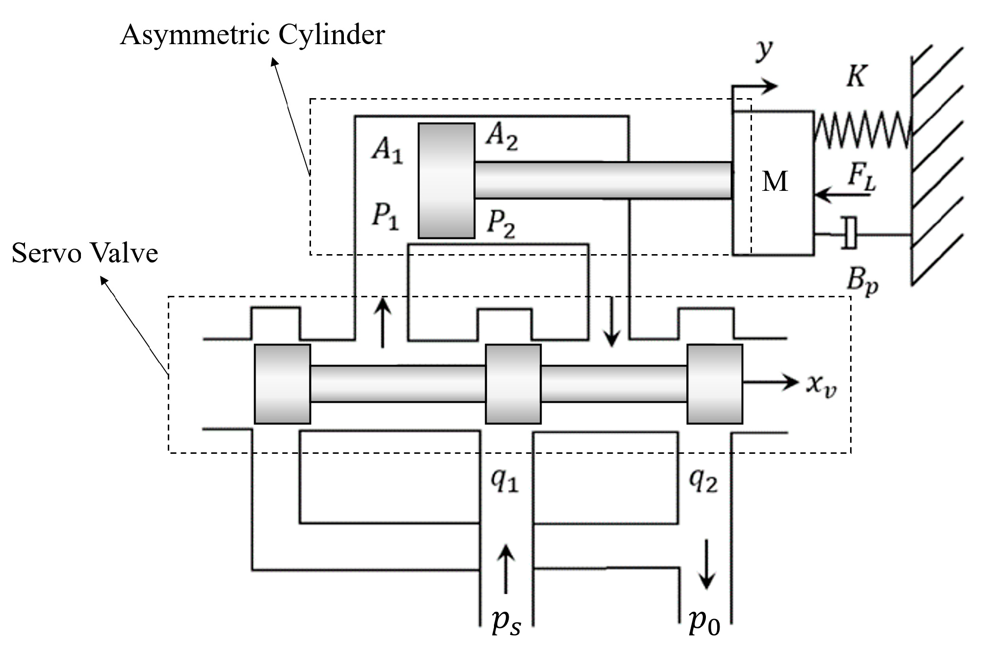
3.2. Modeling of Asymmetric Cylinder Controlled by Servo Valve Subsystem

Figure 8 shows the schematic diagram of the asymmetric cylinder controlled by the valve subsystem, and the direction of the arrow shown is the positive direction of each variable. By establishing the subsystem model of the asymmetric cylinder controlled by the servo valve, the quantitative relationship between the spool displacement $x_v$ and the piston displacement $y$ of the hydraulic cylinder can be obtained.

For the purpose of further analysis, the following assumptions are established: the servo valve is paired with an asymmetric cylinder; the internal and external leakage of the hydraulic cylinder is assumed to be laminar; the connecting pipeline between the servo valve and the hydraulic cylinder is characterized as short and thick, with the dynamic characteristics of the pipeline and pressure losses being disregarded; the supply pressure $p_s$ of the subsystem is considered constant, while the return pressure $p_0=0$; and the influences of temperature and liquid compressibility on the entire subsystem are neglected. The following discussion focuses on the process in which the servo valve spool moves to the right and the hydraulic cylinder piston extends to the right [32].

When the servo valve spool is shifted to the right, i.e., $x_v>0$, the flow equation of the servo valve is:

$$q_1=w{x}_v{C}_d\sqrt{{\displaystyle \frac{2}{\rho }}(p_s-p_1)}$$

(16)

$$q_2=w{x}_v{C}_d\sqrt{{\displaystyle \frac{2}{\rho }}{p}_2}$$

(17)

where $q_1$ is the rodless chamber flow rate of hydraulic cylinder, $q_2$ is the rod-end chamber flow rate of hydraulic cylinder, $p_1$ is the pressure in the rodless chamber of the hydraulic cylinder, $p_2$ is the pressure in the rod-end chamber of the hydraulic cylinder, $p_s$ is the pressure of the hydraulic source, $C_d$ is the flow coefficient, $w$ is the area gradient of the servo valve orifice, $\rho$ is the density of hydraulic fluid, and $x_v$ is the spool displacement.

Considering the process of the piston extending after the hydraulic cylinder is subjected to hydraulic pressure, the hydraulic cylinder inlet chamber flow rate $q_1$ and return chamber flow rate $q_2$ are:

$$q_1={\displaystyle \frac{{\mathrm{d}V}_1}{\mathrm{d}t}}+C_{\mathit{ip}}\left(p_1 -p_2\right)+C_{\mathit{ep}}{p}_1+{\displaystyle \frac{V_1}{{\beta }_e}}{\displaystyle \frac{{\mathrm{d}p}_1}{\mathrm{d}t}}$$

(18)

$$q_2={\displaystyle \frac{{\mathrm{d}V}_2}{\mathrm{d}t}}+C_{\mathrm{ip}}\left(p_1-p_2\right)-C_{\mathit{ep}}{p}_1-{\displaystyle \frac{V_2}{{\beta }_e}}{\displaystyle \frac{{\mathrm{d}p}_2}{\mathrm{d}t}}$$

(19)

where $C_{\mathit{ip}}$ is the internal leakage coefficient of the hydraulic cylinder, $C_{\mathit{ep}}$ is the external leakage coefficient of the hydraulic cylinder, and ${\beta }_e$ is the bulk elastic modulus.

Notice that when ignoring the compressibility of the hydraulic fluid and hydraulic cylinder leakage, according to Equations (16)–(19), there are:

$$q_1={\displaystyle \frac{\mathrm{d}{V}_1}{\mathrm{d}t}}=A_1{\displaystyle \frac{\mathrm{d}y}{\mathrm{d}t}}=w{x}_v{C}_d\sqrt{{\displaystyle \frac{2}{\rho }}(p_s -p_1)}$$

(20)

$$q_2={\displaystyle \frac{\mathrm{d}{V}_2}{\mathrm{d}t}}=A_2{\displaystyle \frac{\mathrm{d}y}{\mathrm{d}t}}=w{x}_v{C}_d\sqrt{{\displaystyle \frac{2}{\rho }}{p}_2}$$

(21)

where $A_1$ is the effective area of piston side, $A_2$ is the piston area on the rod side, and $y$ is the piston displacement.

From Equations (20) and (21):

$$n={\displaystyle \frac{q_2}{q_1}}={\displaystyle \frac{A_2}{A_1}}=\sqrt{{\displaystyle \frac{p_2}{p_s -p_1}}}<1$$

(22)

Ideally, the output power $N_L$ of the servo valve and the output power $N_{\mathit{out}}$ of the hydraulic cylinder are equal, i.e.,:

$$N_L=p_L{q}_L=F_{L}v=N_{\mathit{out}}$$

(23)

where $p_L$ is the load pressure, $q_L$ is the load flow, $F_L$ is the external load force, and $v$ is the piston speed.

According to the force analysis of the piston in Figure 8, there is:

$$F_L=p_1{A}_1-p_2{A}_2$$

(24)

The speed of the piston of the hydraulic cylinder is:

$$v={\displaystyle \frac{q_1}{A_1}}={\displaystyle \frac{q_2}{A_2}}$$

(25)

Associating Equations (23)–(25), we obtain:

$$p_L{q}_L=\left(p_1{A}_1-p_2{A}_2\right){\displaystyle \frac{q_1}{A_1}}=\left(p_1-p_2{\displaystyle \frac{A_2}{A_1}}\right)q_1=(p_1- n{p}_2)q_1$$

(26)

The load pressure is defined as follows:

$$p_L={\displaystyle \frac{F_L}{A_1}}={ {\displaystyle \frac{p_1{A}_1-p_2{A}_2}{A_1}}=p}_1-n{p}_2$$

(27)

From Equations (26) and (27):

$$q_L=q_1$$

(28)

Associating Equations (22) and (28), we obtain:

$$p_1={\displaystyle \frac{n^3{p}_s+p_L}{1+n^3}},p_2={\displaystyle \frac{n^2(p_s -p_L)}{1+n^3}}$$

(29)

From Equations (18), (28), and (29):

$$q_L=q_1=A_1{\displaystyle \frac{d_y}{\mathit{dt}}}+C_{\mathit{ie}}{p}_L+C_f{p}_s+{\displaystyle \frac{V_t}{4{\beta }_e}}{\displaystyle \frac{{\mathit{dp}}_L}{\mathit{dt}}}$$

(30)

where $C_{\mathit{ie}}$ is the equivalent leakage coefficient, $C_f$ is the additional leakage coefficient, and $V_t$ is the equivalent total volume.

When the piston extends, all output forces and load forces of the hydraulic cylinder should be in a state of force balance, hence, it follows that:

$$p_1{A}_1-p_2{A}_2=p_L{A}_1=m_t{\displaystyle \frac{d^{2}y}{{\mathit{dt}}^2}}+B_p{\displaystyle \frac{\mathit{dy}}{\mathit{dt}}}+\mathit{Ky}+F_L$$

(31)

where $m_t$ is the total mass translated to the piston, $B_p$ is the total viscous damping coefficient, and $K$ is the load spring stiffness.

In order to conduct a linear analysis of the system, nonlinear load forces and the like must be neglected. Therefore, based on the flow characteristics of fluids through small orifices, Equation (16) is linearized under small perturbations, simplifying to:

$$q_L=q_1=K_q{x}_v-K_c{p}_L$$

(32)

where $K_q$ is the flow gain, and $K_c$ is the flow-pressure coefficient.

Applying the Laplace transform to Equations (30), (31), and (32), and simplifying, we obtain the following mathematical model with input as the spool displacement and external load and output as the hydraulic cylinder piston displacement:

$$Y(S)={\displaystyle \frac{\frac{K_q}{A_1}{X}_v-\frac{K_{\mathit{ce}}}{{A_1}^2}(1+\frac{V_t}{4{\beta }_e{K}_{\mathit{ce}}}S)F_L}{S(\frac{S^2}{{{\omega }_h}^2}+\frac{{2\xi }_h}{{\omega }_h}S+1)}}$$

(33)

where ${\omega }_h$ is the natural frequency, $K_{\mathit{ce}}$ is the total flow-pressure coefficient ($K_{\mathit{ce}}=K_c+C_{\mathit{ie}}$), and ${\xi }_h$ is the hydraulic damping ratio (${\xi }_h={\displaystyle \frac{K_{\mathit{ce}}}{A_1}}\sqrt{{\displaystyle \frac{{\beta }_e{m}_t}{V_t}}}+{\displaystyle \frac{B_p}{{4A}_1}}\sqrt{{\displaystyle \frac{V_t}{{\beta }_e{m}_t}}}$). Therefore, the transfer function of the hydraulic cylinder displacement $Y($S) to the spool displacement $X_v$ is:

$${\displaystyle \frac{Y(S)}{X_v}}={\displaystyle \frac{\raisebox{1ex}{$K_q$}\!\left/ \!\raisebox{-1ex}{$A_1$}\right.}{S(\frac{S^2}{{{\omega }_h}^2}+\frac{2{\xi }_h}{{\omega }_h}S+1)}}$$

(34)

The transfer function of the hydraulic cylinder displacement $Y($S) to the interference force $F_L$ is:

$${\displaystyle \frac{Y\left(S\right)}{F_L}}={\displaystyle \frac{- \frac{K_{\mathit{ce}}}{{A_1}^2}(1+\frac{V_t}{4{\beta }_e{K}_{\mathit{ce}}}S)}{S(\frac{S^2}{{{\omega }_h}^2}+\frac{{2\xi }_h}{{\omega }_h}S+1)}}$$

(35)

3.3. Modeling of Servo Valve Displacement Sensor Subsystem

As an essential component for the implementation of negative feedback automatic control in servo valves, the displacement sensor transforms the input displacement signal from the hydraulic cylinder piston into a voltage signal, which is then output to the electrical components of the servo valve. The mathematical model of the displacement sensor is:

$$U_f\left(S\right)=Y{K}_f$$

(36)

where $U_f$ is the output voltage, $K_f$ is the gain of the displacement sensor and $Y$ is the displacement of hydraulic cylinder piston.

3.4. Modeling of Hydraulic Drive System

By assembling the servo valve mechatronics subsystem, the asymmetric cylinder controlled by the servo valve subsystem, and the servo valve displacement sensor subsystem, the overall mathematical model of the hydraulic transmission system can be obtained. By combining Equations (14), (15), and (34)–(36), the open-loop transfer function of the system is obtained:

$$G(S)H(S)={\displaystyle \frac{K_V}{S(\frac{S^2}{{{\omega }_{\mathit{sv}}}^2}+\frac{{2\xi }_{\mathit{sv}}}{{\omega }_{\mathit{sv}}}S +1)(\frac{S^2}{{{\omega }_h}^2}+\frac{2{\xi }_h}{{\omega }_h}S +1)}}$$

(37)

where $K_V$ is the open-loop amplification factor ($K_V=K_f{K}_{\mathit{sv}}{K}_f/A_1$).

Subsequently, modeling was carried out using the Simulink component of MATLAB R2022b, according to Equation (37), and the model created by Simulink is shown in Figure 9.

The parameter values in

Table 3. Calculated parameters and values.

Parameters	Symbol (Unit)	Values
External load equivalent mass	$m_t(\mathrm{kg})$	400
Flow rate	$n$	0.61
Total flow-pressure coefficient	$K_{\mathit{ce}}({\mathrm{m}}^5/\mathrm{N}·\mathrm{s})$	$6.45\times {10}^{-12}$
Hydraulic damping ratio	${\xi }_h$	0.25

were used in the further analysis of the model.

The external load equivalent mass in Table 3 is the total mass of the hydraulic cylinder and the pulley block. This is because their motions are translational, and there is no rotational inertia, so we modeled them using 3D modeling software SOLIDWORKS 2022, which, subsequently, showed the total mass. In addition, the flow rate, the total flow-pressure coefficient, and the hydraulic damping ratio were obtained using the calculations of Equations (22) and (33), respectively.

Stability is one of the most critical characteristics of a control system and an essential condition for its normal operation. Any system will deviate from its original equilibrium state under the influence of disturbances, resulting in an initial deviation. Stability refers to the system’s ability to return to the original equilibrium state from the initial deviation state after the disturbance has subsided. If the system’s dynamic process gradually decays and tends to zero over time, it is considered stable; conversely, if the system’s dynamic process diverges over time under the influence of disturbances, the system is deemed unstable. The system’s characteristic equation was assessed in the time domain using the Routh stability criterion. If all coefficients of the characteristic equation are positive, the system can be determined to be in a stable state.

According to the formula:

$$2{\xi }_h{\omega }_h>K_v$$

(38)

Substituting the data gives:

$$2\times 0.25\times 268=134>0.523$$

(39)

Thus, it can be determined that the hydraulic transmission system of the penetration unit is stable and possesses a significant gain margin.

In the frequency domain, system stability was analyzed by plotting the amplitude and phase frequency response curves, with relative stability in the frequency domain referred to as the stability margin, commonly quantified by the phase margin and the gain margin [33]. The condition for system stability typically requires a phase margin between 30 deg and 60 deg and a gain margin greater than 6 dB. Consequently, the stability of the system can be analyzed through its open-loop frequency characteristics [34,35]. Given the open-loop transfer function, the open-loop Bode plot can be obtained using MATLAB/Simulink R2022b simulation analysis to determine the system’s gain and phase margins. The Bode plot for Equation (37) is shown in Figure 10:

From Figure 10, it is evident that the system’s gain margin is 44.8 dB, and the phase margin is 62.5 degrees, thus meeting the stability requirements and exhibiting excellent stability. Under the condition without a controller, a unit step signal was applied to the system to observe its transient response. The simulation was performed on the model, as shown in Figure 9, and the results are shown in Figure 11 and Figure 12.

As depicted in Figure 11, upon the application of a unit step input to the system, the displacement response exhibits the following characteristics: the response time is moderate, ranging from 3 to 4 s, yet overshoot is observed, which is detrimental to practical engineering applications. Furthermore, according to the prevailing standards both domestically and internationally, the penetration rate should be controlled within a range of 2 cm/s ± 10%. The velocity of the hydraulic transmission system illustrated in Figure 12 clearly fails to meet these requirements. Consequently, it is imperative to incorporate a controller into the original system for regulation.

The hydraulic transmission system employs a PID (Proportional Integral Derivative) control algorithm, combined with negative feedback control methods, to effectively stabilize the penetration rate under conditions of uncertain soil parameters [36]. The transfer function of the PID control algorithm is represented as follows:

$${\displaystyle \frac{I(s)}{e(s)}}=K_p+K_i{\displaystyle \frac{1}{s}}+K_{d}s$$

(40)

where $K_p$ is the proportional gain, $K_i$ is the integral gain, $K_d$ is the derivative gain, $I(s)$ is the input, and $e(s)$ is the error. The complete model of the hydraulic transmission system after adding the PID controller is shown in Figure 13.

3.5. Determination of System Boundary Conditions

In the field of hydraulic transmission, the hydraulic cylinder crawling phenomenon is prevalent, characterized by non-uniform motion, intermittent stops, and erratic speed variations during low-speed operation. This instability and discontinuity in movement arise from unstable flow to or from the actuator, manifesting as intermittent flow disruptions. Particularly at low speeds, the phenomenon can range from subtle vibrations to significant jumps, severely impacting the stability and control precision of the hydraulic system. As detailed in Table 1, while maintaining a constant penetration speed of 2 cm/s, the stroke of the hydraulic cylinder increases with higher gear positions, inversely reducing its movement velocity. By decreasing the hydraulic cylinder’s speed, one can identify the onset of sudden velocity changes, indicative of the crawling phenomenon, thus revealing the rig’s speed lower limit.

The hydraulic transmission system depicted in Figure 13, augmented with a PID controller, was configured with fixed parameters. By gradually reducing the system’s speed, we obtained the outcomes presented in Figure 14. Observations reveal that at a set speed of 0.38 cm/s for the hydraulic cylinder, the crawling phenomenon emerges, failing to satisfy the precision requirements for penetration speed. Consequently, the maximum stroke amplification ratio of the hydraulic cylinder is limited to five, per the velocities detailed in Table 1; thus, the system is capped at a maximum of five gears.

4. Discussion

To verify whether the adaptive CPT system can shift gears based on dynamic loads, thereby achieving maximum single-penetration travel under load conditions, a model with time-varying dynamic loads was subjected to simulation experiments to discuss the model’s stability under load disturbances. As a reference for calculating the dynamic loads, a set of in situ test data was selected from the reference literature 37. These resistance data were chosen because they represent the typical variation in the sediment resistance during the penetration of the rod.

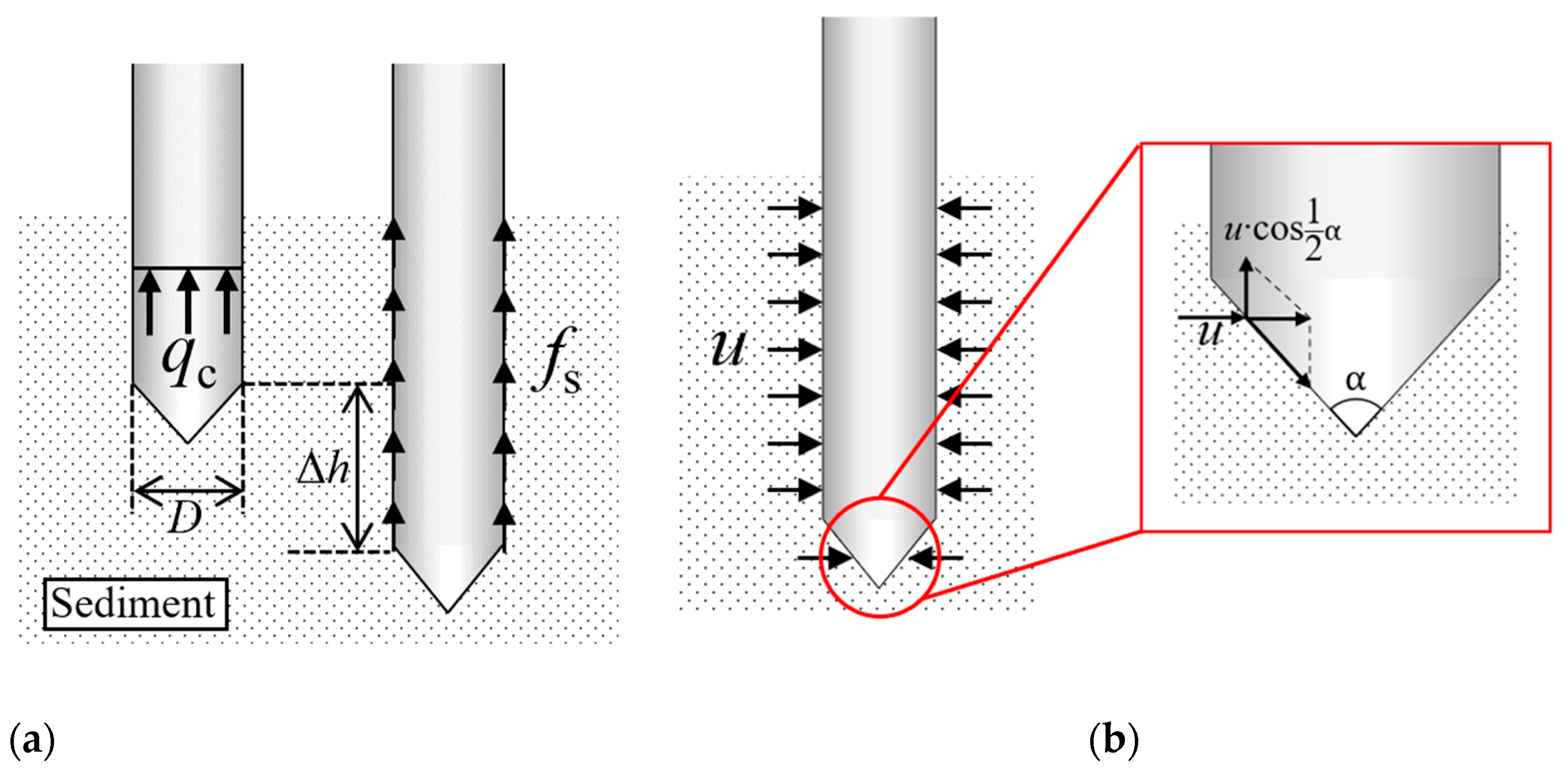
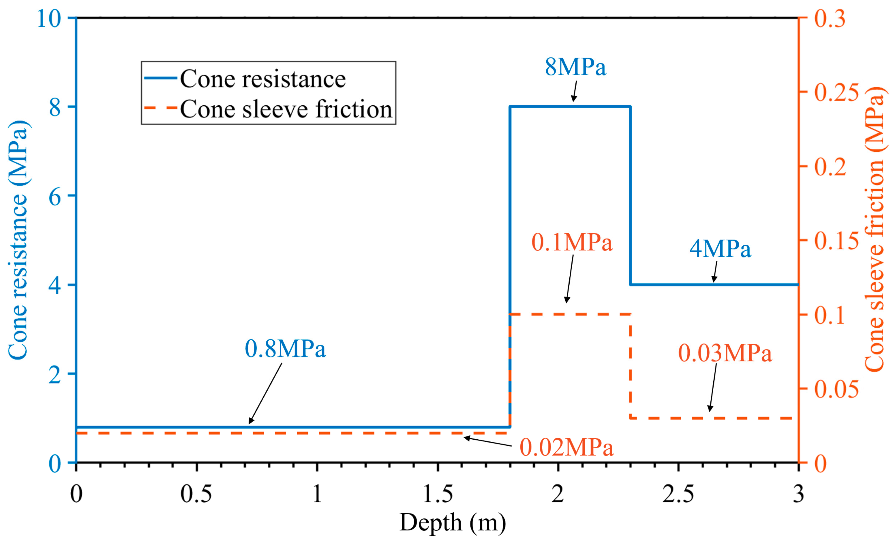
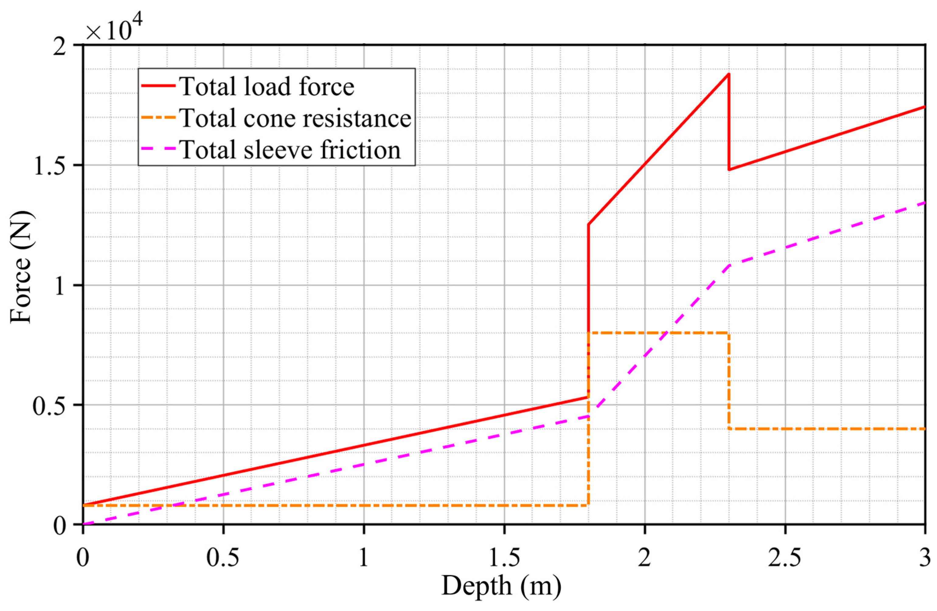
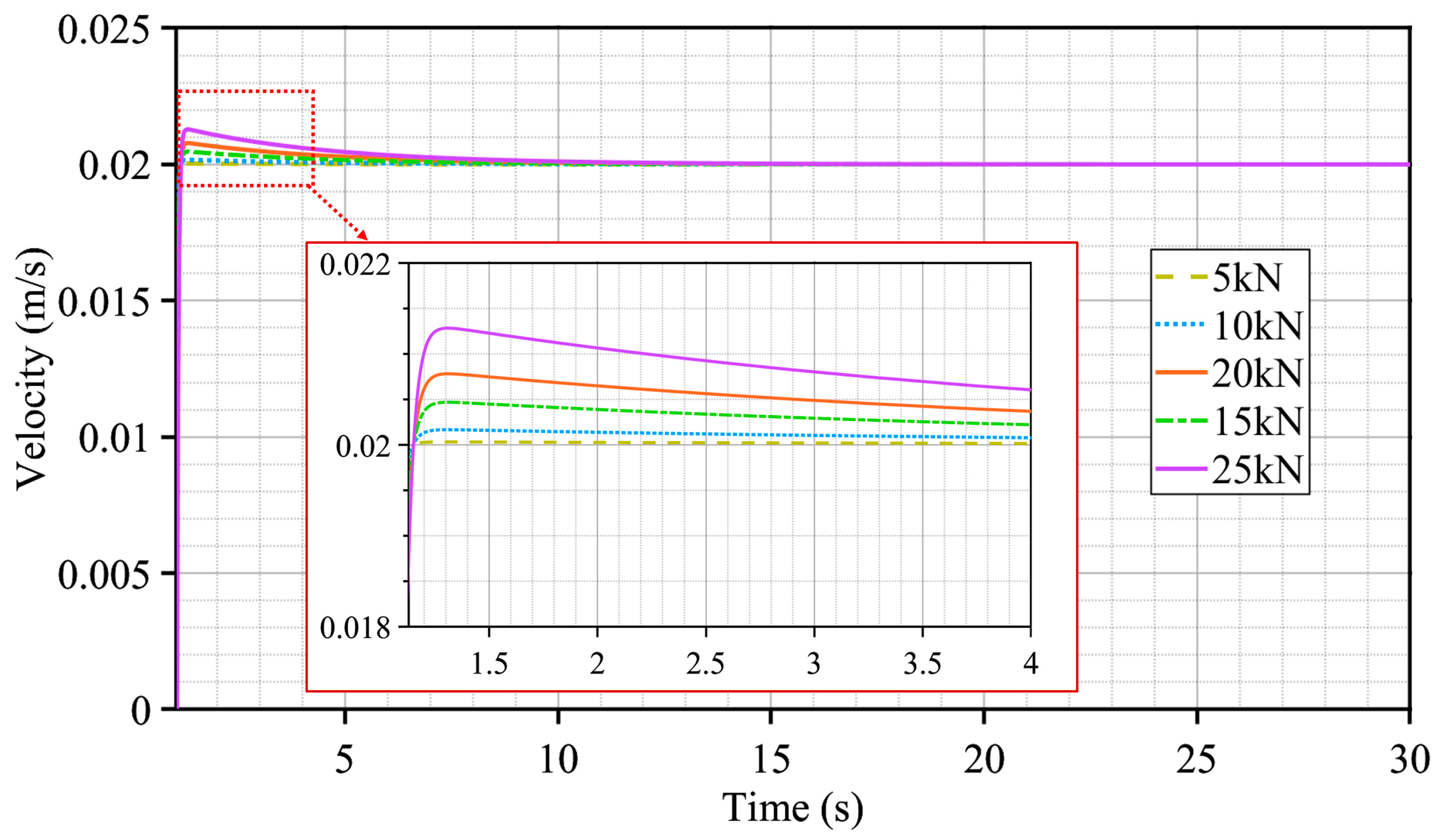
4.1. Calculation of Dynamic Load

To optimize the design of the transmission system for achieving uniform penetration of the rod, it is essential to analyze the patterns of load variation experienced by the rod during sediment penetration and determine the correlation between the penetration depth of the rod and the penetration load. The mechanics of this penetration are highly complex, with factors influencing the resistance to penetration in marine sediments, including the substrate type, penetration depth, water content, porosity, and wet density.

With the development of domestic and international CPT rigs and the urgent need for marine engineering construction, the use of CPT in marine engineering surveys has increased significantly, generating a substantial amount of measured data. These data provide strong support for studying the correlation between CPT data and soil physical–mechanical parameters. Wei Duan and colleagues [37] conducted a total of 383 seabed CPTU tests at the site of the Hong Kong–Zhuhai–Macao Bridge in the Pearl River Delta using Fugro Seacalf equipment, obtaining the relationship between cone resistance and sleeve friction varying with depth within a 53 m depth range beneath the seabed. The results of their tests are shown in Figure 15.

From the figure, it can be observed that both cone resistance and sleeve friction gradually increase with penetration depth within the same soil layer, with significant changes occurring at soil boundary areas. When the soil transitions from soft clay to clay–sand mixtures, there is a sharp increase in cone resistance, rising from approximately 0.8 MPa to about 8 MPa. Upon reaching the sand layer, the value continues to increase uniformly to over 15 MPa.

Due to the complexity and uncertainty of submarine geological conditions, the rod may penetrate strata of varying hardness during penetration, and the resistance it encounters will change with the depth of penetration and the type of soil layer. Consequently, the load on the hydraulic transmission system varies over time, leading to unstable penetration speeds. In actual penetration processes, the total resistance experienced by the rod, as shown in Figure 16a, primarily consists of the total cone resistance $Q_c$ and the total sleeve friction force $F_f$, which can be calculated by Equations (41) and (42). In addition, as shown in Figure 16b, since the pore water pressure is mainly horizontal and only a vertical component exists at the tip of the cone, which has a very small effect on the vertical motion of the rod, it is ignored in the following analysis in order to simplify the model:

$$Q_c=q_c·A$$

(41)

$$F_f=f_s·A_h$$

(42)

where $q_c$ is the cone resistance, $f_s$ is the sleeve friction, $A$ is the area of the tip of the cone, and $A_h$ is the total area of the rod sleeve in contact with the soil.

Thus, the total penetration resistance F_t is obtained:

$$F_t=Q_c+F_s=q_c·A+f_s·A_h=q_c·A+{\mathsf{\Sigma }f}_s·\mathrm{\pi }·D·∆h$$

(43)

where $D$ is the rod diameter ($D\approx 40 \mathrm{mm}$), and $∆h$ is the depth of penetration of the rod.

Referencing the in situ test data illustrated in Figure 15, this paper selected a soil sample segment transitioning from soft clay to clay–sand mixtures. Due to the significant changes in the relevant parameters associated with soil type variations, such typical data can effectively test the robustness of the control system. Subsequently, the data were simplified to meet the design and simulation requirements of the penetration unit and hydraulic transmission system, predicting the changes in cone resistance and sleeve friction during the penetration process [38,39]. The organized data are presented in Figure 17, showing the curves of cone resistance and sleeve friction as a function of depth. Following this, using Equation (43), the variation curve of the hydraulic cylinder load force was calculated and is depicted in Figure 18.

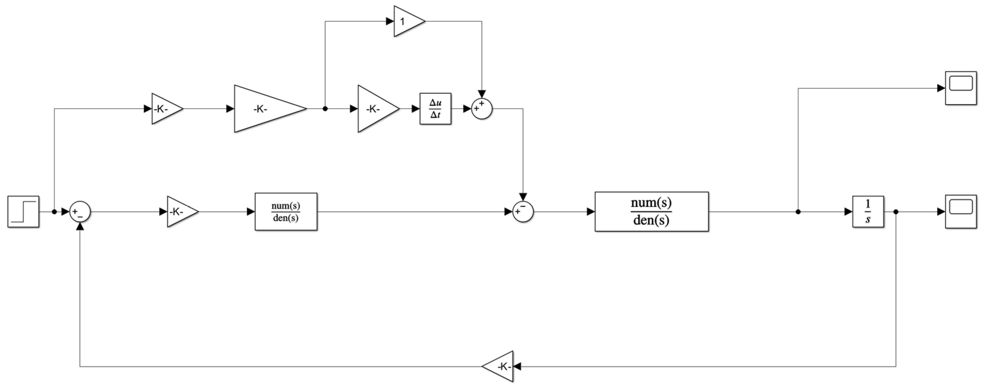
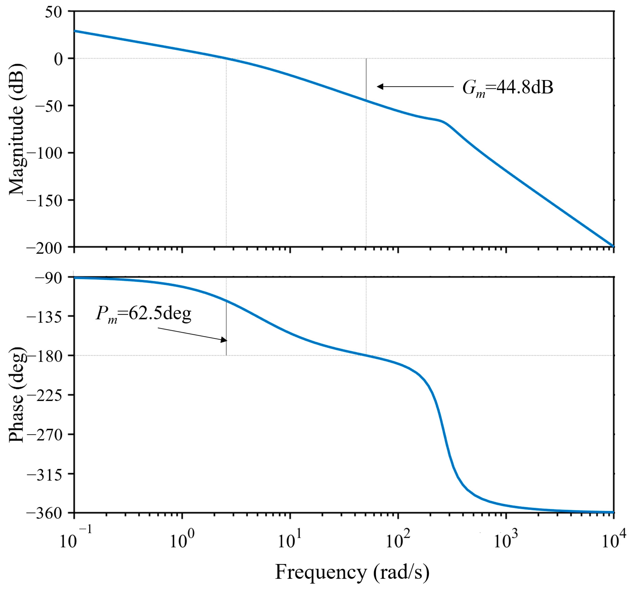
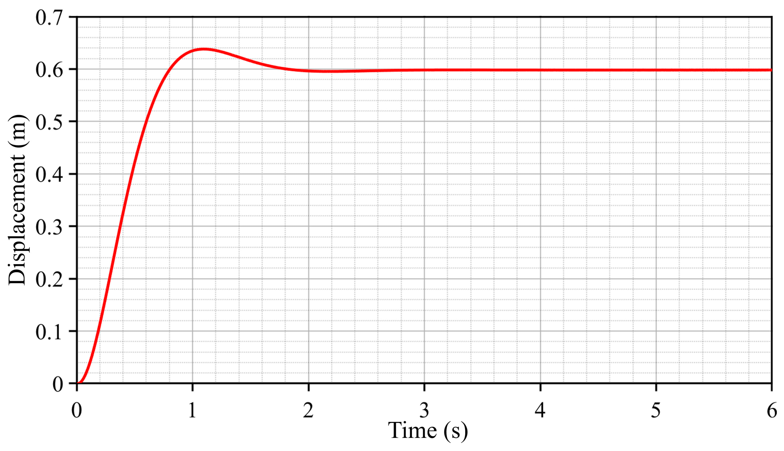
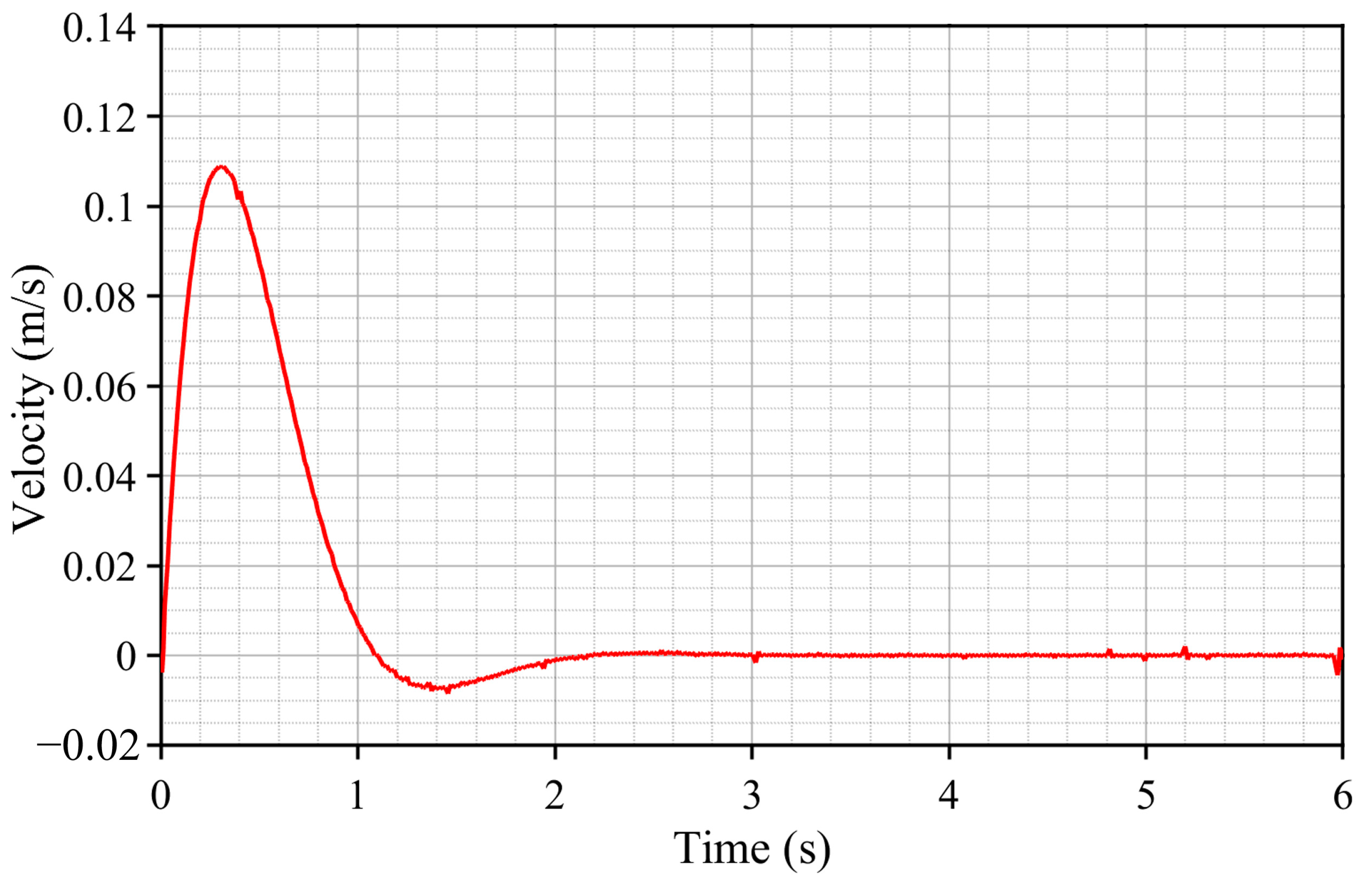
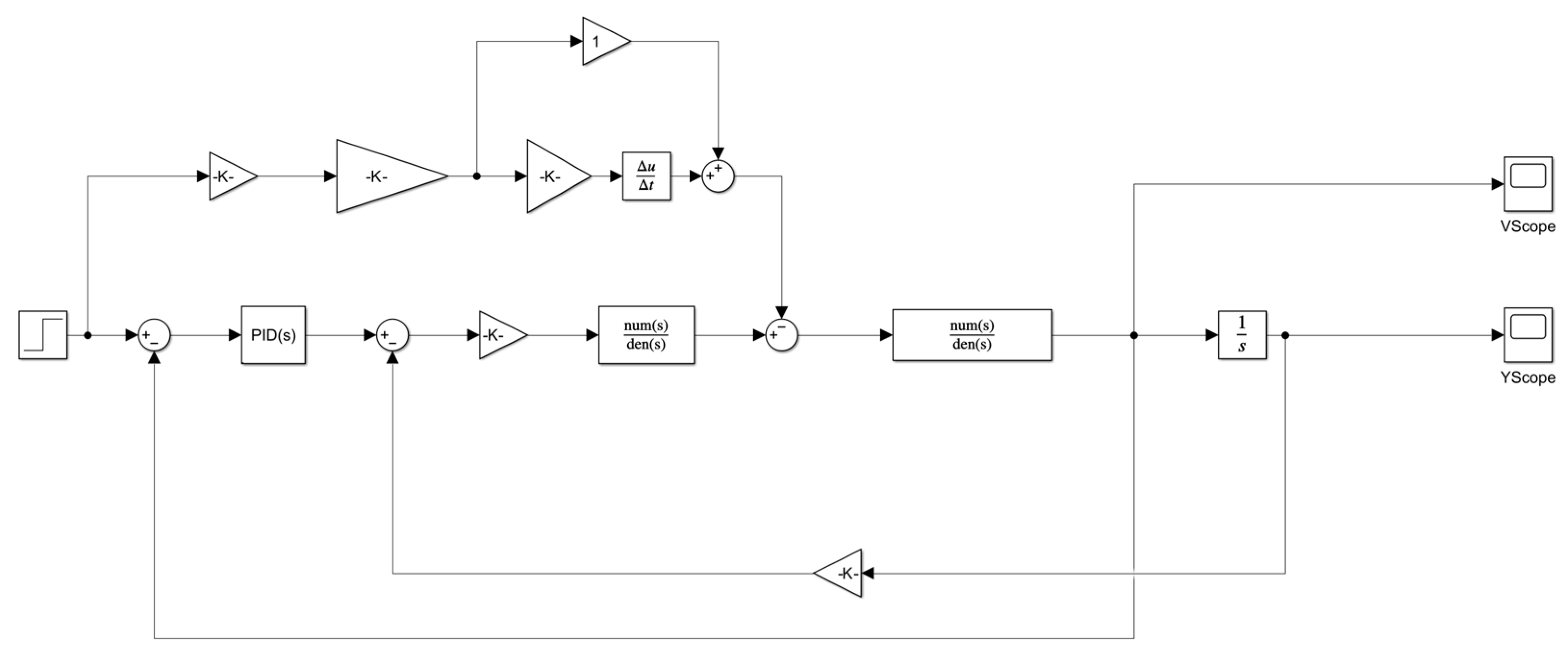
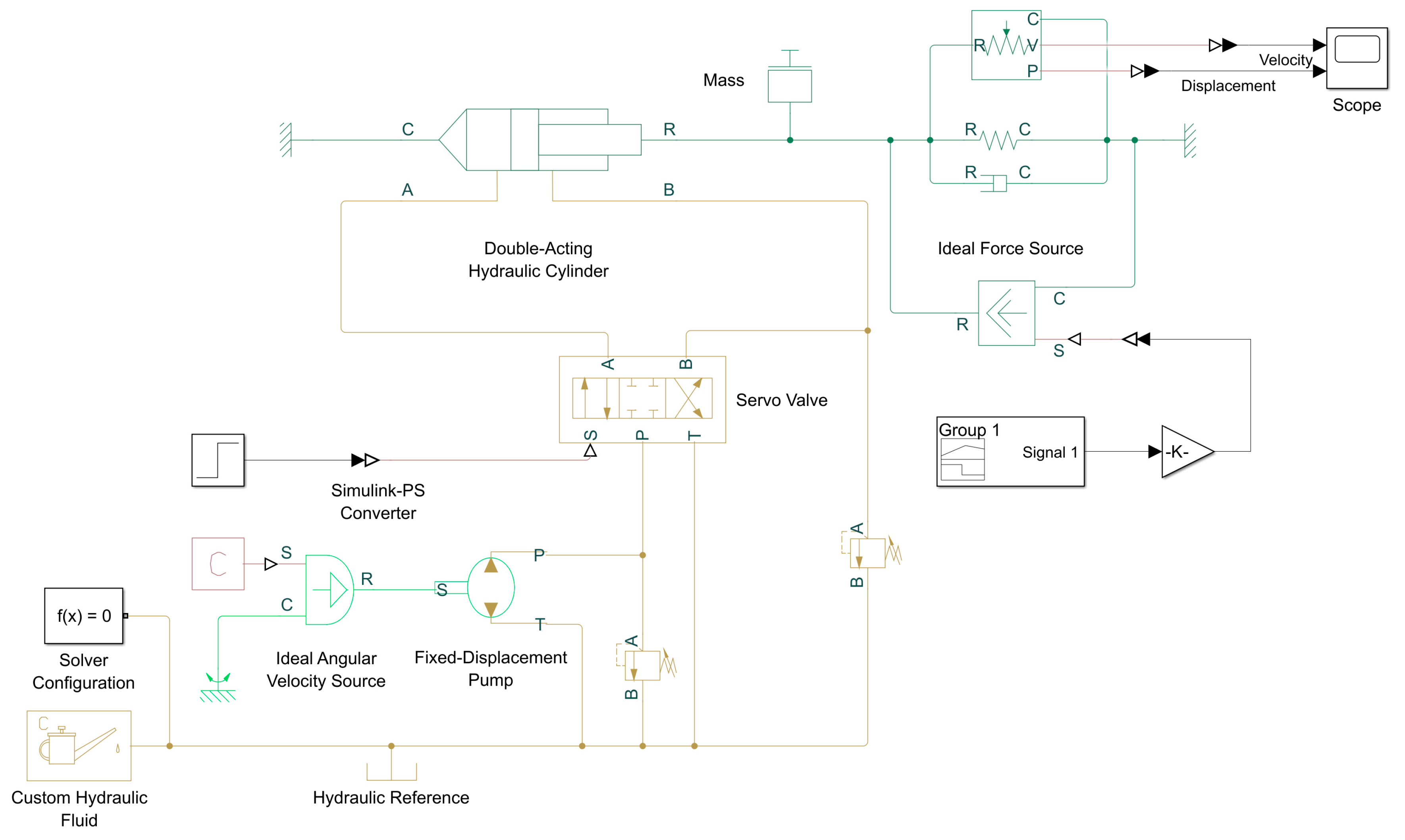
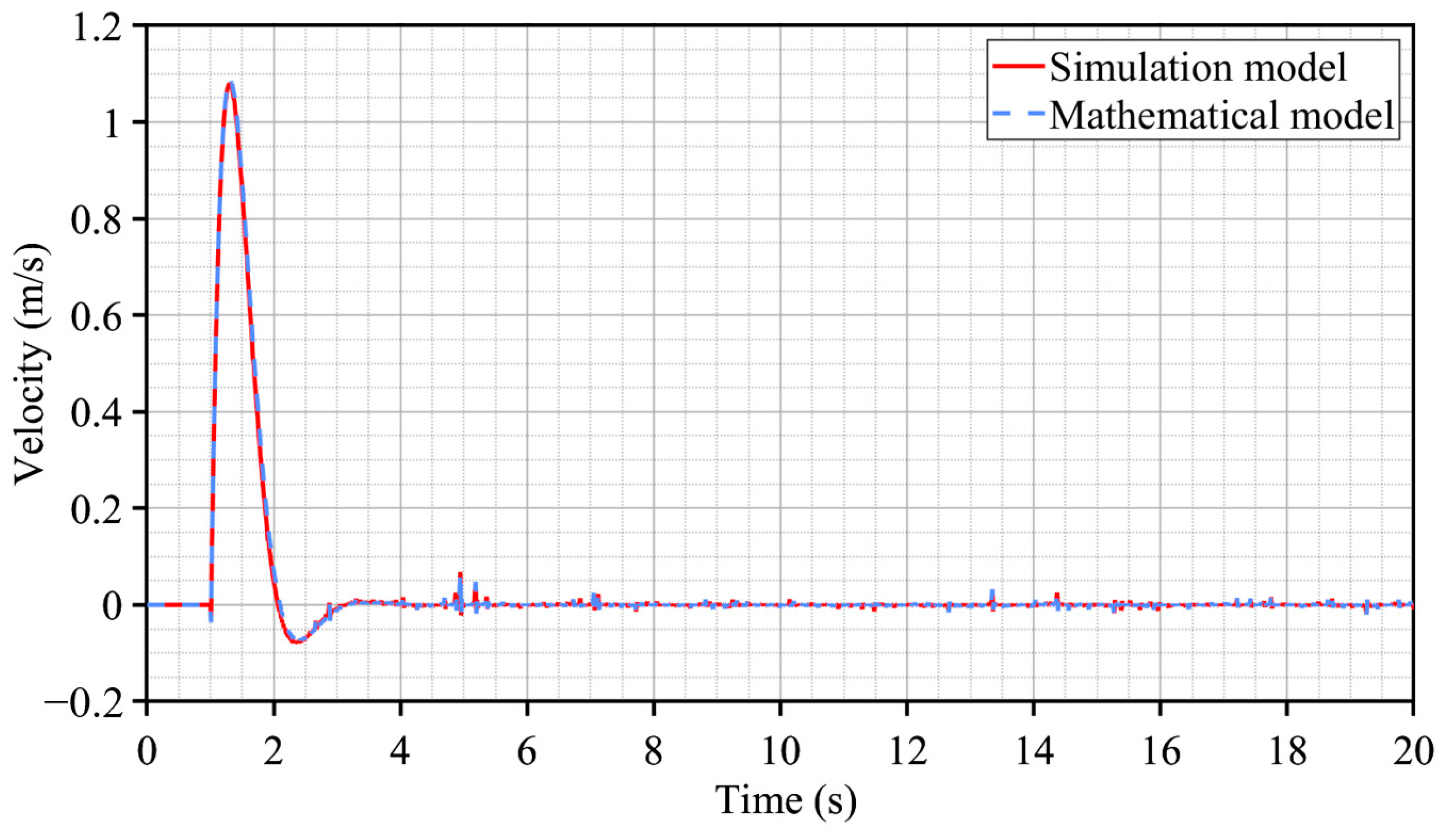
4.2. Model Consistency Validation and Control Logic Design

To achieve the adaptive function of maximizing single-penetration travel under load conditions, we first utilized the Simscape library in MATLAB/Simulink R2022b to construct a simulation model. This model was then compared with the simulation results of the mathematical model shown in Figure 9 to verify the consistency between the two. Subsequently, the adaptive gear-shifting control logic was programmed using Stateflow.

Simscape, a powerful multi-domain physical system modeling and simulation library introduced by MathWorks, enables the rapid creation of physical simulation models within the Simulink environment. By employing component models based on physical connections and physics-to-Simulink signal conversion modules, Simscape allows physical models to integrate and interact directly with other component libraries, facilitating the modeling, control, and co-simulation of hydraulic systems. The hydraulic transmission system simulation model established using Simscape is depicted in Figure 19.

The parameter values used in the aforementioned physical model are consistent with those in Table 2. The simulation results of this model were compared with the outcomes of the mathematical model presented in Figure 9. As shown in Figure 20, the velocity profiles of the hydraulic cylinder piston essentially overlap, validating the mathematical model.

Subsequently, the load-adaptive shifting module was designed using Stateflow, with the fundamental logic being that during startup, the fifth gear is used for penetration operations. When sensors detect an external load exceeding the nominal load range or when the safety valve in the hydraulic system overflows, the gripping mechanical hand pauses and resets. It then sequentially downshifts until a new gear can overcome the external load, after which operations resume. The following candlestick chart is used to represent the design loads corresponding to the five gears, as shown in Figure 21, where the red upper shadow indicates the maximum load corresponding to the gears, and the real body represents the nominal load.

As can be seen, a load margin of 2 kN is reserved for each gear position, which is a safety redundancy designed to take into account the response time of the system. In addition, the load ranges corresponding to two neighboring gears are partially overlapped, which ensures the movement of the clamping manipulator during the gear shift is as smooth as possible. Next, the designed adaptive gearshift module, PID controller, and simulation model were assembled to form the complete system, as shown in Figure 22.

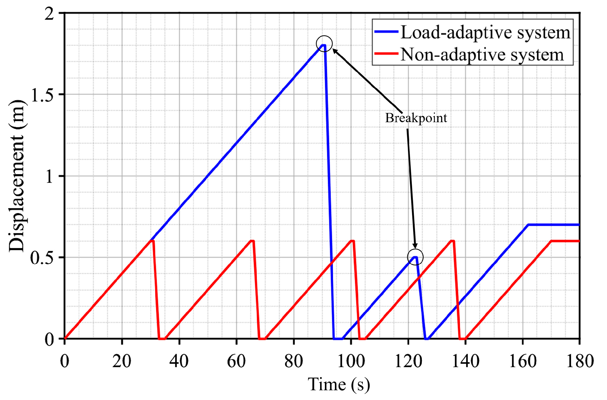
4.3. Static Load Testing

In order to test and validate the performance of the PID controller, the system model was simulated after applying 5 kN, 10 kN, 15 kN, 20 kN, and 25 kN static loads sequentially. The simulation results are shown in Figure 23.

The results indicate that system velocity oscillations amplify with escalating external loads, peaking at an overshoot when subjected to an external load of 25 kN. However, under PID controller regulation, system velocity remains consistently within the specified tolerance of 2 cm/s ± 10%, satisfying the design specifications.

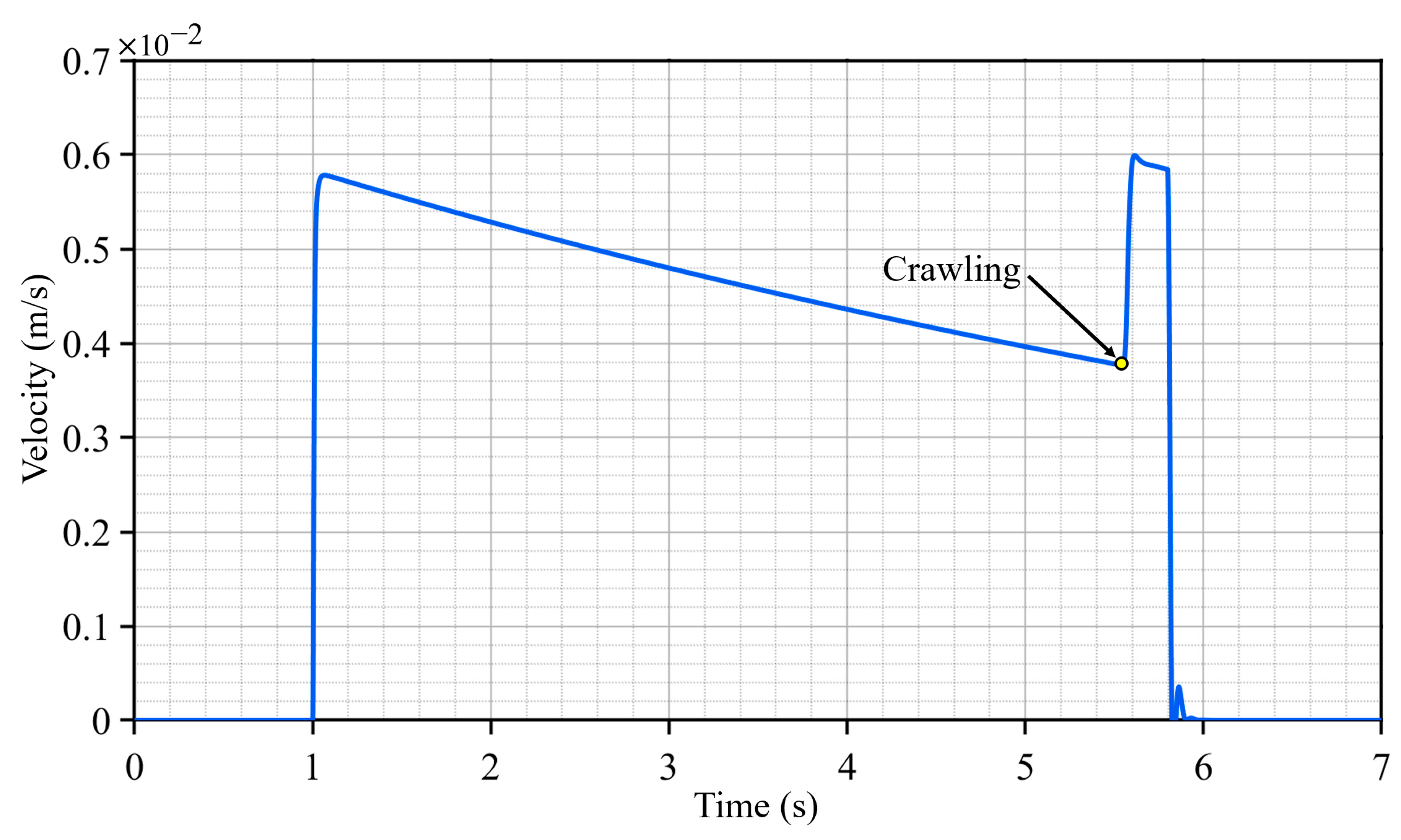
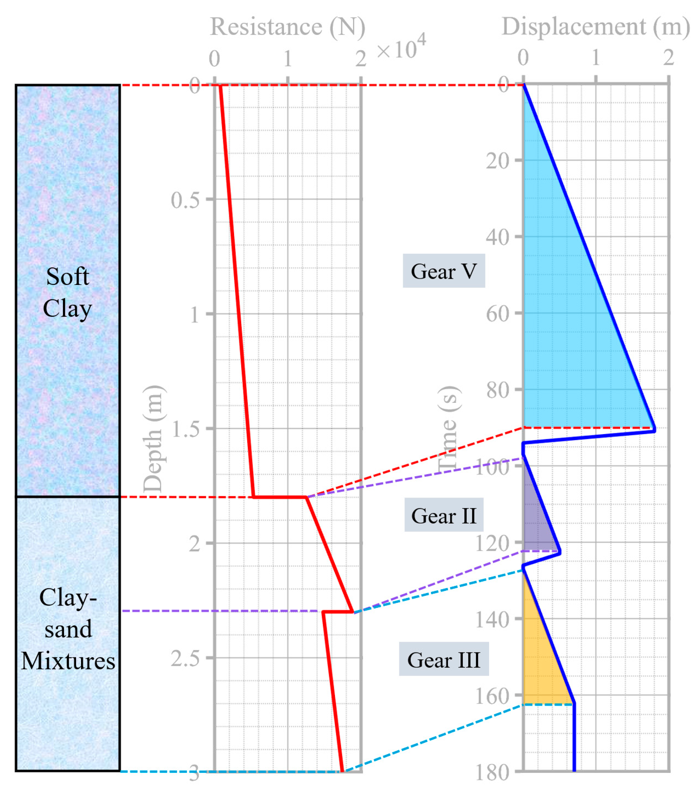
4.4. Dynamic Load Testing

The dynamic load presented in Figure 18 was applied to both the adaptive CPT system designed in this study and the standard CPT system (disabled adaptive functions, with a fixed single penetration stroke of 0.6 m), with a target penetration depth of 3 m set for the simulation. As shown in Figure 24, the figure indicates that the adaptive CPT system, when set to a penetration depth of 3 m, performed a total of three penetration operations, taking 170 s in total, whereas the standard non-adaptive CPT system, due to its fixed 0.6 m stroke, executed six penetration operations, taking 180 s in total. Additionally, the simulation results of the adaptive CPT system were compared with the soil layer data, as depicted in Figure 25. The comparison reveals that for a penetration depth of 0–1.8 m, the soil type is soft clay with minimal resistance, prompting the system to automatically shift to the fifth gear, achieving a single penetration stroke of 1.8 m. When the depth is between 1.8 and 2.3 m, the system encounters the boundary between soft clay and clay–sand mixtures, where the penetration resistance peaks at 18,000 N, causing the system to switch to the second gear for penetration. For depths between 2.3 and 3 m, the soil type transitions entirely to clay–sand mixtures, with resistance slightly decreasing and stabilizing, leading the system to shift to the third gear to complete the remaining penetration.

Tests found that load-adaptive CPT reduced data breakpoints by 50% from four to two for the same external load compared to traditional CPT. In addition, in the depth range of 0 to 1.8 m, the adaptive CPT system obtained a maximum single penetration stroke of 1.8 m due to the smaller external load. In summary, the load-adaptive CPT system flexibly shifts gears in response to external loads, achieving maximum single-penetration strokes and overcoming load forces more efficiently than conventional CPT systems. It demonstrates superior penetration continuity and operational efficiency, requiring fewer penetration attempts under identical resistance conditions.

5. Conclusions

This paper addresses issues with the sediment cone penetration test by proposing a novel load-adaptive sediment CPT rig. This rig is designed to maximize single-penetration strokes under conditions that overcome sediment resistance, minimize zero-rate conditions, and ensure data continuity. The rig’s penetration unit, driven by a hydraulic cylinder and pulley-block system, amplifies the penetration stroke. The clamping manipulator’s flexibility in accommodating rods and sediment sensors of various diameters enhances the CPT rig’s environmental adaptability, enriches test data, and better supports sedimentology research.

This paper analyzed the mechanical properties and layering patterns of sediment, along with the interaction mechanisms between sediment and mechanical structures. Subsequently, a mathematical model of a mechanical structure–sediment-integrated system was established using MATLAB/Simulink R2022b software. We also confirmed the model’s boundary conditions through a comprehensive analysis of sediment characteristics and the hydraulic system. To facilitate system function design, we developed a physical simulation model, conducted comparative tests between the physical and mathematical models, and further designed a load-adaptive control logic to form a complete model.

This study simulated and tested the mechanical structure–sediment-integrated model using real sediment test data from the Pearl River Delta estuary (the Hong Kong–Zhuhai–Macao Bridge site). The results indicate that the rig in this paper exhibits superior continuity and operational efficiency under identical penetration resistance conditions when compared to conventional CPT rigs. In low-resistance sediment layers, it automatically shifts to a higher gear, employing minimal penetration force for maximum single-stroke penetration while ensuring data continuity and conserving energy. Conversely, when encountering abrupt sediment resistance fluctuations, the rig downshifts to deliver increased penetration force, and the hydraulic system stabilizes the rod’s speed to maintain accuracy. Thus, the novel load-adaptive CPT rig and its mechanical structure–sediment model emerge as an innovative option for subsea geological investigations and sedimentology research.

References

1. Wang, J.; Tang, G.; Huang, J.X. Analysis and modelling of a novel hydrostatic energy conversion system for seabed cone penetration test rig. Ocean. Eng. 2018, 169, 177–186. [Google Scholar] [CrossRef]
2. Douglas, B.J. Soil classification using electric cone penetrometer. In Proceedings of the Sympsium on Cone Penetration Testing and Experience, Geo-Technical Engineering Division, ASCE, St. Louis, MO, USA, 26–30 October 1981. [Google Scholar]
3. Wahl, D.A.J. Implementation of Variable Rate Cone Penetration Testing: An Experimental Field Study; University of California: Davis, CA, USA, 2012. [Google Scholar]
4. Ghose, R.; Goudswaard, J. Integrating S-wave seismic-reflection data and cone penetration test data using a multiangle multiscale approach. Geophysics 2004, 69, 440–459. [Google Scholar] [CrossRef]
5. White, D.J. CPT equipment: Recent advances and future perspectives. Cone Penetration Test. 2022, 2022, 66–80. [Google Scholar]
6. Ji, F.D.; Jia, Y.G.; Liu, X.L.; Guo, L.; Zhang, M.S.; Shan, H.X. In situ measurement of the engineering mechanical properties of seafloor sediment. Mar. Geol. Quat. Geol. 2016, 36, 191–200. [Google Scholar]
7. Luo, T.; Song, Y.; Zhu, Y.; Liu, W.; Liu, Y.; Li, Y.; Wu, Z. Triaxial experiments on the mechanical properties of hydrate-bearing marine sediments of South China Sea. Mar. Pet. Geol. 2016, 77, 507–514. [Google Scholar] [CrossRef]
8. Ma, H.; Zhou, M.; Hu, Y.; Hossain, M.S. Effects of cone tip roughness, in-situ stress anisotropy and strength inhomogeneity on CPT data interpretation in layered marine clays: Numerical study. Eng. Geol. 2017, 227, 12–22. [Google Scholar] [CrossRef]
9. Lunne, T.; Robertson, P.K.; Powell, J.J.M. Cone penetration testing in geotechnical practice. Eng. Geol. 1999, 50, 219–220. [Google Scholar]
10. Robertson, P.K. Soil classification using the cone penetration test. Can. Geotech. J. 1990, 27, 151–158. [Google Scholar] [CrossRef]
11. Yin, K.S.; Zhang, L.M.; Wang, H.J.; Zou, H.F.; Li, J.H. Marine soil behaviour classification using piezocone penetration test (CPTu) and borehole records. Can. Geotech. J. 2021, 58, 190–199. [Google Scholar] [CrossRef]
12. Wang, C.; Guo, L.; Jia, L.; Sun, W.; Xue, G.; Yang, X.; Liu, X. Development and application of a 3,000-m Seabed Cone Penetration Test and Sampling System based on a hydraulic drive. Front. Mar. Sci. 2024, 11, 1377405. [Google Scholar] [CrossRef]
13. Storteboom, O.; Woollard, M.; Verhagen, J. Efficiency examined of hands-free Cone Penetration Testing using the SingleTwist™ with COSON. In Cone Penetration Testing 2022; CRC Press: Boca Raton, FL, USA, 2022; pp. 230–235. [Google Scholar]
14. Shoukat, G.; Michel, G.; Coughlan, M.; Malekjafarian, A.; Thusyanthan, I.; Desmond, C.; Pakrashi, V. Generation of Synthetic CPTs with Access to Limited Geotechnical Data for Offshore Sites. Energies 2023, 16, 3817. [Google Scholar] [CrossRef]
15. Lunne, T. The CPT in offshore soil investigations–a historic perspective. JK Mitchell Lecture. In Proceedings of the 2nd International Symposium on the Cone Penetration Test, CPT, Huntington Beach, CA, USA, 9–11 May 2010; p. 10. [Google Scholar]
16. Randolph, M.F. New tools and directions in offshore site investigation. Aust. Geomech. J. 2016, 51, 81–92. [Google Scholar]
17. Robertson, P.K. Cone penetration test (CPT)-based soil behaviour type (SBT) classification system—An update. Can. Geotech. J. 2016, 53, 1910–1927. [Google Scholar] [CrossRef]
18. Lu, Y.; Duan, Z.; Zheng, J.; Zhang, H.; Liu, X.; Luo, S. Offshore cone penetration test and its application in full water-depth geological surveys. In IOP Conference Series: Earth and Environmental Science; IOP Publishing: Bristol, UK, 2020; Volume 570, p. 042008. [Google Scholar]
19. Qiao, H.; Liu, L.; He, H.; Liu, X.; Liu, X.; Peng, P. The practice and development of T-bar penetrometer tests in offshore engineering investigation: A comprehensive review. J. Mar. Sci. Eng. 2023, 11, 1160. [Google Scholar] [CrossRef]
20. McCALLUMA, A. Cone penetration testing (CPT) in Antarctic firn: An introduction to interpretation. J. Glaciol. 2014, 60, 83–93. [Google Scholar] [CrossRef]
21. McCALLUMA, A. A brief introduction to cone penetration testing (CPT) in frozen geomaterials. Ann. Glaciol. 2014, 55, 7–14. [Google Scholar] [CrossRef]
22. Ghanizadeh, A.R.; Aziminejad, A.; Asteris, P.G.; Armaghani, D.J. Soft Computing to predict earthquake-induced soil liquefaction via CPT results. Infrastructures 2023, 8, 125. [Google Scholar] [CrossRef]
23. Cui, Y.; Guo, L.; Liu, T.; Yang, Z.; Ling, X.; Yang, X.; Lu, K.; Xue, G. Development and application of the 3000 m-level multiparameter CPTu in-situ integrated test system. Mar. Georesources Geotechnol. 2023, 41, 400–411. [Google Scholar]
24. Robertson, P.K.; Cabal, K.L. Guide to Cone Penetration Testing for Geotechnical Engineering; Gregg Drilling & Testing: Signal Hill, CA, USA, 2015. [Google Scholar]
25. Du, Y.; Zhu, L.; Zou, H.; Zhang, L.; Cai, G.; Liu, S. Evaluation of CPTU-based soil classification charts for offshore sediments in Pearl River Delta, China. In Proceedings of the Geo-Congress 2020, Minneapolis, Minnesota, 25–28 February 2020; American Society of Civil Engineers: Reston, VA, USA, 2020; pp. 633–639. [Google Scholar]
26. Khosravi, A.; Martinez, A.; DeJong, J.T. Discrete element model (DEM) simulations of cone penetration test (CPT) measurements and soil classification. Can. Geotech. J. 2020, 57, 1369–1387. [Google Scholar] [CrossRef]
27. Jia, R.; Hino, T.; Chai, J.; Yoshimura, M. Interpretation of density profile of seabed sediment from nuclear density cone penetration test results. Soils Found. 2013, 53, 671–679. [Google Scholar] [CrossRef]
28. Fudong, J.; Yonggang, J.; Xiaolei, L. Development and application of new offshore CPT equipment. Coast. Eng. 2016, 35, 1–9. [Google Scholar]
29. Krage, C.P.; DeJong, J.T.; Schnaid, F. Estimation of the coefficient of consolidation from incomplete cone penetration test dissipation tests? J. Geotech. Geoenvironmental Eng. 2015, 141, 06014016. [Google Scholar] [CrossRef]
30. de Lange, D.A.; van Duinen, T.A.; Peters, D.J. Large diameter cone penetrometers: What is an appropriate location for the transition to the rod diameter. In Cone Penetration Testing 2022; CRC Press: Boca Raton, FL, USA, 2022; pp. 127–132. [Google Scholar]
31. Niazi, F.S.; Mayne, P.W. Cone penetration test based direct methods for evaluating static axial capacity of single piles. Geotech. Geol. Eng. 2013, 31, 979–1009. [Google Scholar] [CrossRef]
32. Zhang, S.; Li, S.; Minav, T. Control and performance analysis of variable speed pump-controlled asymmetric cylinder systems under four-quadrant operation. Actuators 2020, 9, 123. [Google Scholar] [CrossRef]
33. Ma, Y.; Gu, L.C.; Xu, Y.G.; Shi, L.C.; Wang, H.T. Research on control strategy of asymmetric electro-hydraulic servo system based on improved PSO algorithm. Adv. Mech. Eng. 2022, 14, 16878132221096226. [Google Scholar] [CrossRef]
34. Krishnamurthy, V.; Seshadri, V. Model reduction using the Routh stability criterion. IEEE Trans. Autom. Control. 1978, 23, 729–731. [Google Scholar] [CrossRef]
35. Kim, S.D.; Cho, H.S.; Lee, C.O. Stability analysis of a load-sensing hydraulic system. Proc. Inst. Mech. Eng. Part A Power Process Eng. 1988, 202, 79–88. [Google Scholar] [CrossRef]
36. Margolis, D.L.; Hennings, C. Stability of hydraulic motion control systems. ASME. J. Dyn. Sys., Meas., Control. 1997, 119, 605–613. [Google Scholar] [CrossRef]
37. Duan, W.; Congress, S.S.C.; Cai, G.; Puppala, A.J.; Dong, X.; Du, Y. Empirical correlations of soil parameters based on piezocone penetration tests (CPTU) for Hong Kong-Zhuhai-Macau Bridge (HZMB) project. Transp. Geotech. 2021, 30, 100605. [Google Scholar] [CrossRef]
38. Cui, G.; Li, Y.; Pei, W. The effect of natural water content on the penetration resistance of seabed sediment. Hydrogr. Surv. Charting 2005, 6, 51–53. [Google Scholar]
39. Xue, G.; Liu, Y.; Guo, L.; Liu, B. Optimization on motion-robust and energy-saving controller for hydraulic penetration system of seabed equipment. Proc. Inst. Mech. Eng. Part M J. Eng. Marit. Environ. 2021, 235, 792–808. [Google Scholar] [CrossRef]
Figure 1. Diagram of the load-adaptive CPT rig.
Water 17 01159 g001
Figure 2. Diagram of the penetration unit.
Water 17 01159 g002
Figure 3. Schematic diagram of the transmission.
Water 17 01159 g003
Figure 4. Diagram of the composition of the pulley block.
Water 17 01159 g004
Figure 5. Schematic diagram of 1st gear movement.
Water 17 01159 g005
Figure 6. Schematic diagram of 2nd gear movement.
Water 17 01159 g006
Figure 7. Schematic diagram of 3rd gear movement.
Water 17 01159 g007
Figure 8. Schematic diagram of asymmetric cylinder controlled by servo valve subsystem.
Water 17 01159 g008
Figure 9. Mathematical modeling of hydraulic transmission system in Simulink.
Water 17 01159 g009
Figure 10. Bode plot for Equation (37).
Water 17 01159 g010
Figure 11. Output displacement of the system under a unit step signal input.
Water 17 01159 g011
Figure 12. Output velocity of the system under a unit step signal input.
Water 17 01159 g012
Figure 13. Diagram of complete model of the hydraulic drive system.
Water 17 01159 g013
Figure 14. Speed in case of crawling phenomenon of hydraulic cylinder.
Water 17 01159 g014
Figure 15. In situ CPT data referenced from Duan W et al. 37.
Water 17 01159 g015
Figure 16. Force analysis diagram of the rod. (a) Cone resistance and sleeve friction. (b) Pore water pressure.
Water 17 01159 g016
Figure 17. Depth–cone resistance curve and depth–cone sleeve friction curve.
Water 17 01159 g017
Figure 18. Depth–load force curves.
Water 17 01159 g018
Figure 19. Simulation model of a hydraulic transmission system in Simulink using Simscape.
Water 17 01159 g019
Figure 20. Comparison of the results of simulation model with results of mathematical model.
Water 17 01159 g020
Figure 21. Design loads for each gear.
Water 17 01159 g021
Figure 22. Complete hydraulic transmission system.
Water 17 01159 g022
Figure 23. Velocity of the system obtained by simulation under different static loads.
Water 17 01159 g023
Figure 24. Comparison between load-adaptive CPT system and non-adaptive CPT system.
Water 17 01159 g024
Figure 25. Simulation results of load-adaptive CPT system compared with soil resistance.
Water 17 01159 g025