Research on Flood Forecasting in the Pa River Basin Based on the Xin’anjiang Model

Abstract

This study explores flood forecasting in the Pa River basin, a major tributary of the Beijiang River in South China, by integrating the Xin’anjiang hydrological model with the Shuffled Complex Evolution-University of Arizona (SCE-UA) algorithm for parameter calibration. Fifteen observed flood events from April to August 2024 were employed in this study, with twelve events used for model calibration and the remaining three for validation. Additionally, to assess model performance under extreme conditions, a 50-year return period flood event from June 2020 was incorporated as a supplementary validation case. The calibrated model reproduced flood hydrographs with high accuracy, achieving Nash–Sutcliffe Efficiency (NSE) values of up to 0.98, relative peak discharge errors generally within ±10%, and peak timing deviations under 3 h. The validation results demonstrated consistent performance across both typical and extreme events, indicating that the proposed framework provides a feasible and physically interpretable approach for flood forecasting in data-limited catchments.

1. Introduction

Hydrological forecasting methodologies have transitioned through three distinct paradigms: empirical-statistical approaches [1], physically based modeling [2,3], and hybrid intelligent systems [4], reflecting a progression from data-driven correlations to mechanistic process analysis. Early empirical-statistical methods relied on historical hydrometeorological correlations but suffered from oversimplified representations of rainfall runoff mechanisms. The late 20th century saw advancements in distributed physically based models (e.g., HEC-HMS, SWAT) [5], which spatially discretized basins and integrated atmospheric, pedological, and vegetative dynamics. However, these models faced operational constraints due to dependencies on high-resolution geospatial inputs (e.g., DEMs, soil taxonomy) and computationally intensive simulations [6,7]. Contemporary hybrid systems synergize machine learning with multi-source data assimilation (satellite observations, IoT networks), enhancing nonlinear process characterization and operational forecasting robustness [5].

The Xin’anjiang model is a watershed hydrological model that was originally designed for application in humid and semi-humid regions [8]. This model embodies a conceptual-physical methodology within the physically based modeling paradigm. Its architecture integrates saturation-excess runoff mechanisms via modular soil moisture dynamics and runoff partitioning schemes, whereas simplified parameterization strategies ensure computational tractability. This semi-distributed framework achieves a balance between mechanistic process emulation and operational efficiency, thereby differentiating it from purely data-driven statistical approaches and data-intensive machine learning hybrids. This model is classified as a conceptual-physical framework, reflecting its dual emphasis on structural process representation and practical applicability. It is particularly suited for medium-sized watersheds, where constrained observational data necessitate a careful balance between physical fidelity and predictive efficiency [9].

The SCE-UA (Shuffled Complex Evolutionary Algorithm), a hybrid evolutionary optimization framework integrating composite strategies [10], is widely implemented in hydrological and environmental sciences for parameter calibration [11]. Combining the advantages of Simulated Annealing (SA) and Evolutionary Algorithms (EA) [12], it employs population clustering, complex evolution, and information recombination mechanisms to efficiently optimize highly nonlinear, non-convex objective functions [13]. The algorithm exhibits self-adaptive sampling, self-tuning control parameters [14], and dynamic global-local search equilibrium, demonstrating robust convergence and computational stability in resolving high-dimensional parameter identification problems across hydrological models.

Recent studies have explored diverse directions to enhance hydrological forecasting accuracy, such as integrating optimization algorithms into physically based models, improving hazard response simulations, and combining AI with numerical weather models. For example, Wang et al. (2024) demonstrated that coupling the distributed Xin’anjiang model with a Particle Swarm Optimization algorithm improved simulation fidelity in a semi-humid basin [15]. Huang et al. (2025) investigated dam-break flood impacts on slope stability, highlighting the practical importance of accurately capturing flood dynamics [16]. Xu et al. (2025) proposed an AI-driven regional forecasting framework for typhoons, which emphasizes the value of combining data-driven systems with process-based models [17]. These advances reflect a growing interest in hybrid or multi-source approaches. However, for lumped hydrological models such as Xin’anjiang, there remains a need for targeted and interpretable frameworks that support event-wise calibration and sensitivity-aware parameterization, especially under data-limited conditions [18].

Integrating the SCE-UA algorithm with the Xin’anjiang model addresses critical challenges in hydrological parameter optimization, including high dimensionality, nonlinearity, and parameter equifinality [19]. The SCE-UA framework prioritizes explicit preservation of physical consistency during parameter identification for conceptual hydrological models, whereas machine learning techniques focus on advanced feature importance analysis through automated pattern recognition. Its independence from large training datasets significantly reduces the computational demands. This contrasts with data-driven feature selection in machine learning, which may compromise physical interpretability when handling the Xin’anjiang model’s modular structure, requiring explicit representation of soil moisture dynamics and runoff partitioning. Other optimization algorithms, such as gradient descent methods, are prone to local optima stagnation due to their dependency on initial conditions and directional sensitivity in non-convex parameter spaces. This inherent limitation stems from their deterministic search trajectories, which often terminate prematurely at saddle points or shallow minima without exploring globally optimal regions. As a global optimization framework, SCE-UA enhances the model’s ability to escape local optima and identify physically consistent parameters across diverse hydrological regimes [20], thereby improving simulation reliability [21]. The SCE-UA algorithm achieves significantly faster convergence than genetic algorithms in high-dimensional hydrological parameter optimization while maintaining comparable computational efficiency. The algorithm’s hybrid framework, which systematically combines competitive evolution with complex shuffling, enhances adaptability to basin heterogeneity while sustaining computational efficiency. By mitigating calibration subjectivity and extending applicability to data-limited or morphologically diverse basins, this integrated approach establishes a foundation for watershed analysis amidst environmental change [22,23].

This study aims to enhance flood forecasting accuracy in data-constrained medium watersheds by integrating the Xin’anjiang hydrological model with the SCE-UA optimization algorithm. The main objectives are to (1) enhance model performance under limited data availability, (2) validate simulation accuracy for flood peak timing and hydrograph characteristics using observational data, and (3) demonstrate the model’s adaptability through its application to 16 historical flood events and extreme scenarios, including 5- and 50-year return period floods. The results offer a conceptual framework and methodological reference for future hydrological forecasting and risk evaluation in the Pa River basin.

2. Methodology

This study establishes a structured methodological framework for flood forecasting in the Pa River basin by coupling the Xin’anjiang hydrological model with the Shuffled Complex Evolution-University of Arizona (SCE-UA) global optimization algorithm. The overall workflow includes model configuration, parameter constraint definition based on regional hydrological characteristics, calibration using observed hourly rainfall and discharge records, and validation under both typical and extreme flood scenarios. Twelve measured flood events from 2024 were selected for parameter calibration, and four independent events were used for validation, including an extreme flood that occurred in June 2020 with a 50-year return period. In addition, quantitative sensitivity analysis was conducted to identify key parameters affecting simulation accuracy. The methodological workflow is summarized in Figure 1 and further elaborated in the following subsections.

2.1. Hydrological Model Setup and Parameter Constraints

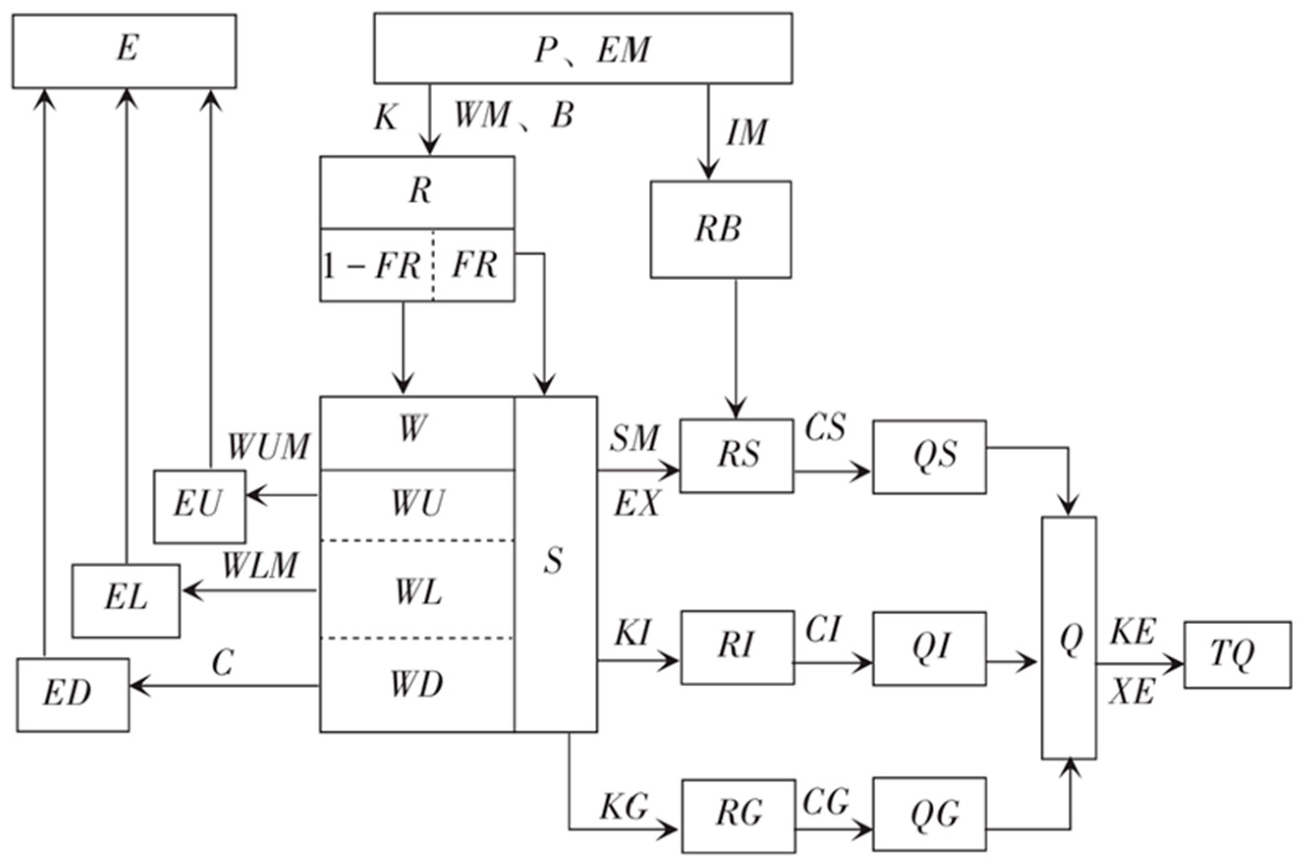
The Xin’anjiang model integrates four physically based modules to simulate hydrological processes: An evapotranspiration module employing a three-layer soil moisture stratification system (upper, lower, and deep zones) that quantifies stratum-specific evaporation–transpiration fluxes; a runoff generation module implementing saturation-excess mechanisms through precipitation–soil moisture coupling [24]; a runoff partitioning module utilizing free water tank drainage principles to differentiate surface, interflow, and groundwater components [15]; and a flow routing module combining linear reservoir methods for slope concentration with Muskingum channel routing for hydrodynamic propagation [25]. This modular architecture enables a precise simulation of basin-scale precipitation–evapotranspiration–runoff interactions through parameterized process coupling, demonstrating superior performance in flood forecasting and water resource allocation applications, with its structural configuration detailed in Figure 2. The parameter definitions of the Xin’anjiang model are presented in

Table 1. The parameter definitions of the Xin’anjiang model.

Abbreviation	Full Name	Description	Abbreviation	Full Name	Description
P	Precipitation	Volume of water falling on the land surface per unit area and time.	IM	Impervious Area Ratio	Fraction of the basin that is impervious, affecting direct runoff.
EM	Water Surface Evaporation	Evaporation rate from open water surfaces.	SM	Free Water Storage Capacity	Capacity of the surface soil layer to store free water before surface runoff occurs.
E	Evapotranspiration	Combined water loss through soil evaporation and plant transpiration.	EX	Exponent of the Free Water Storage Capacity Curve	Influences how free water storage varies across the basin.
R	Runoff from Permeable Areas	Surface flow generated in permeable zones.	KI	Interflow Runoff Coefficient	Regulates the proportion of quick subsurface flow (interflow) contributing to total runoff.
FR	Runoff-Generating Area Ratio	Proportion of basin area contributing to direct runoff.	KG	Groundwater Runoff Coefficient	Determines the fraction of slow baseflow (groundwater flow) contributing to total runoff.
RB	Runoff from Impervious Areas	Surface flow generated in urbanized or impervious zones.	CI	Recession Constant of the Interflow Reservoir	Affects the depletion rate of interflow storage, influencing the recession limb of the hydrograph.
EU/EL/ED	Upper/Lower/Deep-Layer Evapotranspiration	Partitioned evapotranspiration components from soil layers.	CG	Recession Constant of the Groundwater Reservoir	Influences the depletion rate of groundwater storage, affecting baseflow recession.
W	Total Capillary Water Storage	Sum of water held in soil capillary pores.	CS	Recession Constant of the River Network Storage	Controls the attenuation and lag of flow through the river network, impacting flood peak timing and magnitude.
WU/WL/WD	Upper/Lower/Deep-Layer Capillary Water	Water storage in specific soil horizons.	KC	Evapotranspiration Correction Coefficient	Adjusts the potential evapotranspiration rates to better match observed conditions.
S	Surface Free Water Storage	Temporary ponding water before becoming runoff.	KE	Coefficient of Evapotranspiration	Modifies the rate of evapotranspiration, affecting water loss estimates.
RS/RI/RG	Surface Runoff/Interflow/Groundwater Runoff	Three-component runoff generation mechanism.	C	Deep-Layer Evaporation Coefficient	Adjusts evaporation from deeper soil layers, influencing soil moisture dynamics.
B	Exponent of the Tension Water Capacity Curve	Determines the spatial distribution of the tension water capacity.	N	Manning’s Roughness Coefficient	Represents the roughness of the river channel, affecting flow velocity and routing.

.

In this study, we employed the well-established Xin’anjiang model to simulate flood runoff in the Pa River basin. This conceptual rainfall runoff model, grounded in the saturation-excess runoff generation theory, assumes that runoff occurs only when soil moisture reaches field capacity. The model operates on an hourly time step, aligning with the temporal resolution of our input data. We adopted the lumped form of the Xin’anjiang model, treating the entire basin as a single unit characterized by spatially averaged parameters.

The performance of the Xin’anjiang model is highly sensitive to the calibration of its parameters, which govern critical hydrological processes such as runoff generation, infiltration, evapotranspiration, and flow routing [26]. Identifying and constraining these sensitive parameters is essential for enhancing the model’s simulation accuracy. In this study, we focused on calibrating the most sensitive parameters while fixing the less influential ones at values recommended in the literature. A total of 11 parameters were selected for calibration, as shown in

Table 2. Parameter ranges and adjustment rationale for the Xin’anjiang model applied to the Pa River basin.

Parameter	Original Range	Adjusted Range for Pa River	Adjustment Basis
WM	100–300	100–200	The Pa River basin features alluvial plains and weathered sedimentary soils with moderate water-holding capacity.
B	0.1–0.7	0.2–0.6	The basin exhibits heterogeneous soil types and moderate spatial variability in field capacity.
IM	0–0.05	0–0.03	The basin’s substantial forest coverage and limited urbanization result in a low impervious area ratio.
SM	10–50	10–40	The presence of thin soil layers in certain regions leads to reduced water storage capacity.
EX	0.1–1.5	0.1–1.3	The topographic relief and uneven infiltration capacity in the Pa River basin.
KI	0.0–1.0	0.1–1.0	The basin’s permeable soil layers and steep upper catchments facilitate interflow, necessitating a moderately high KI range.
KG	0.0–1.0	0.1–0.8	The fractured bedrock and shallow groundwater table support slow baseflow contribution, reflected in a constrained but active KG range.
CI	0.0–1.0	0.1–0.7	The slope-driven quick response and flash-flood characteristics in the upper basin require tighter control over interflow depletion.
CG	0.0–1.0	0.1–1	Groundwater storage recession is relatively slow.
CS	0.0–1.0	0.01–0.2	Steep flood hydrographs indicate rapid recession, characteristic of the basin’s hydrological response.
KC	0.5–1.5	0.7–1.3	The adjustment reflects the region’s subtropical monsoon climate with high seasonal evapotranspiration variability.

.

During parameter initialization, particular attention was given to the physical relationships and constraints among the parameters. For instance, WM, B, and IM collectively determine the runoff generation characteristics and were adjusted in concert to maintain the model’s physical consistency. Additionally, parameters such as SM, EX, KI, and KG directly influence the runoff and flow routing processes and were set based on the actual conditions of the basin. Through the judicious calibration of these parameters, we aimed to enhance the model’s accuracy in simulating flood events in the Pa River basin.

With the model configured and parameter ranges defined, the next step involved calibrating these parameters using observed flood event data. Each flood event’s input data, including hourly rainfall and initial soil moisture conditions, were used to drive the model. The simulated runoff was then compared to the observed runoff to evaluate the accuracy of a given parameter set. Calibration was approached as an optimization problem, seeking parameter values that best matched the simulated and observed discharge for the calibration events. We employed a global search algorithm to solve this optimization problem, as detailed in the subsequent section.

2.2. Performance Evaluation Metrics

Before launching the parameter calibration, it is essential to define the criteria used to evaluate model performance. This study adopts a multi-faceted evaluation framework, combining deterministic accuracy, hydrograph shape fidelity, and qualitative uncertainty assessment to ensure both numerical precision and hydrological realism [27].

(1)

Deterministic Accuracy Metrics

These indicators assess the agreement between observed and simulated discharge values, particularly focusing on flood peak reproduction and timing alignment:

Nash–Sutcliffe Efficiency ($NSE$):

$$NSE=1-{\displaystyle \frac{{{\displaystyle \sum }}_{i=1}^N{\left[Q_{obs,i}\left(\theta \right)-Q_{sim,i}\left(\theta \right)\right]}^2}{{{\displaystyle \sum }}_{i=1}^N{\left[Q_{obs,i}\left(\theta \right)-{\overline{Q}}_{obs}\right]}^2}}$$

where $Q_{obs,i}$ and $Q_{sim,i}$ represent the observed and simulated discharge values at time I, respectively; ${\overline{Q}}_{obs}$ is the mean observed discharge. $NSE$ values close to 1 indicate high simulation accuracy.

Relative Error of Peak Discharge ($RE$):

$$RE={\displaystyle \frac{Q_{sim,peak}-Q_{obs,peak}}{Q_{obs,peak}}}\times 100\%$$

Capturing flood peak bias as a percentage.

Peak Timing Deviation ($PTD$):

$$PTD=\mid T_{sim,peak}-T_{obs,peak}\mid$$

Measures the absolute difference in hours between the simulated and observed flood peaks.

(2)

Hydrograph Fit Metrics

To evaluate the temporal accuracy and overall runoff response across the event duration, the following error-based metrics are employed:

Mean Absolute Error ($MAE$):

$$MAE={\displaystyle \frac{1}{n}}{\displaystyle \sum }_{i=1}^n\mid Q_{sim,i}-Q_{obs,i}\mid$$

Mean Absolute Relative Error ($MARE$):

$$MARE={\displaystyle \frac{1}{n}}{\displaystyle \sum }_{i=1}^n{\displaystyle \frac{\mid Q_{sim,i}-Q_{obs,i}\mid }{Q_{obs,i}}}\times 100\%$$

These indicators provide a balanced view of simulation quality by combining point-specific and event-scale assessments.

2.3. Calibration Procedure Using SCE-UA

To calibrate the Xin’anjiang model for flood simulation in the Pa River basin, this study implemented SCE-UA, aiming to identify parameter sets that enable an accurate reproduction of observed flood events. The SCE-UA algorithm was specifically chosen for its capacity to efficiently search high-dimensional parameter spaces and avoid local optima, which is critical given the nonlinear and complex behavior of hydrological systems in humid subtropical regions.

2.3.1. Calibration Execution for Each Event

In our study, the SCE-UA algorithm was used to automatically tune the Xin’anjiang model parameters until the simulated flood hydrographs closely matched the observed hydrographs for the calibration events. The calibration procedure was carried out individually for each of the 12 calibration flood events. In other words, for each event, we executed SCE-UA optimization to find an optimal parameter set that reproduces that event’s runoff as accurately as possible. This approach provided a set of candidate parameter sets (one per event), which were later analyzed to select a final representative parameter set for the basin.

The objective function chosen for calibration was the Nash–Sutcliffe Efficiency (NSE), a standard goodness-of-fit metric in hydrology that ranges from −∞ to 1 (with 1 indicating a perfect fit). For each event’s calibration, the algorithm sought to maximize the NSE between observed and simulated runoff; equivalently, the optimization could be formulated as minimizing (1 − NSE) or negative NSE. This metric was chosen for its ability to emphasize the overall hydrograph shape agreement while penalizing large timing and volume errors, which is essential for flood modeling.

2.3.2. Algorithm Configuration and Execution Details

The SCE-UA algorithm was tailored to the calibration requirements of the Xin’anjiang model as follows:

• Parameter Space Definition: Eleven model parameters were subject to calibration. Their initial ranges were set according to the regional hydrological conditions and prior studies.
• Population Initialization: 100 parameter sets were generated using Latin hypercube sampling to ensure broad coverage of the feasible space. Each set represented an 11-dimensional vector.
• Complex Structure: The population was divided into 5 complexes (subpopulations) of 20 parameter sets each, enabling exploration of different solution regions in parallel.
• Evolution and Recombination: Within each complex, 3–5 evolution steps were performed using competitive evolution strategies. Poor-performing members were replaced by new candidates extrapolated from the best performers.
• Shuffling Mechanism: Every 5 iterations, all complexes were merged and globally re-ranked. The updated population was then re-divided into new complexes. This shuffling promoted information exchange and prevented stagnation.
• Convergence Criteria: The calibration for each event continued until either (a) a maximum of 5000 model evaluations was reached or (b) improvement in the best NSE was less than 0.001 over two consecutive shuffling intervals.

2.3.3. Input Parameter Settings and Initialization

• n: Number of decision variables (model parameters) = 11.
• p: Number of complexes = 5 (subpopulations).
• m: Number of points per complex = 20.
• Initial population size: 100 $\left(S=P\times m\right)$ This initial population was generated by Latin hypercube sampling within the specified parameter ranges, ensuring a well-spread and diverse set of trial solutions. Each parameter set is essentially an 11-dimensional vector containing one value for each model parameter (WM, WUM, …, KG, etc.).

2.3.4. Stepwise Calibration

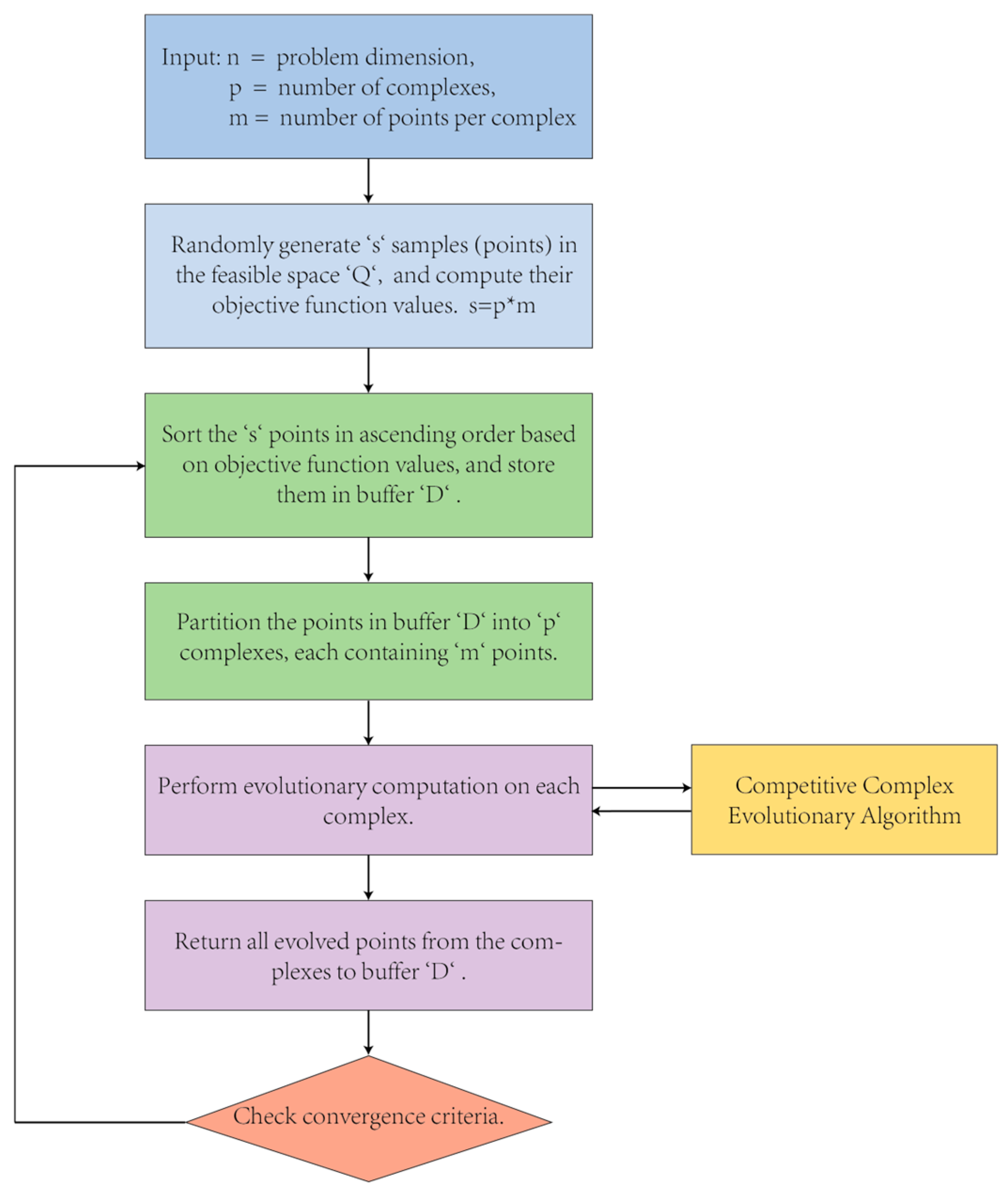
• Step 1: Random Sampling

Generate s = p × m sample points within the feasible parameter space Q. Compute the objective function value for each point.

• Step 2: Sorting and Buffer Initialization

Sort all s points in ascending order based on their objective function values. Store the ranked population in buffer D.

• Step 3: Complex Partitioning

Divide buffer D into p distinct complexes, each containing m points. The partitioning follows a cyclic allocation strategy to maintain diversity (e.g., the k-th complex includes points k, k + p, k + 2p, …).

• Step 4: Evolutionary Computation

For each complex:

Crossover: Recombine high-fitness solutions to exploit local optima.

Mutation: Apply stochastic perturbations to prevent premature convergence.

Evaluate new candidates and update the complex with elite solutions.

• Step 5: Buffer Update

Merge the evolved points from all complexes back into buffer D. Re-sort D based on the updated objective function values.

• Step 6: Convergence Check

The termination criteria for the calibration were defined as follows:

Maximum Number of Model Evaluations: The calibration process was set to terminate if the total number of model evaluations reached 5000. This upper limit was established to prevent excessive computational time and resources.

Convergence Threshold: The calibration would also terminate if the improvement in the objective function became negligible. Specifically, if the change in the best Nash–Sutcliffe Efficiency (NSE) value was less than 0.001 over two consecutive shuffling loops (equivalent to 10 complex iterations), the process was considered to have converged to an optimal solution.

In instances where neither of these conditions was met, the calibration process would continue by returning to step 2 of the SCE-UA algorithm, involving re-sorting and partitioning the population into complexes for further evolutionary search. This iterative refinement ensured a thorough exploration of the parameter space, enhancing the likelihood of identifying the most accurate parameter set for each flood event.

To further evaluate the impact of individual parameters on model output behavior, a quantitative sensitivity analysis was designed and discussed in Section 4.3.

Its computational workflow is illustrated in Figure 3 [28].

3. Study Area Description and Data Preparation

This section describes the spatial and hydrological characteristics of the Pa River basin and details the data sources and event configurations used in model calibration and validation. While the basin is introduced in the study title, the following content provides essential context for interpreting the modeling results, including data preprocessing steps, rainfall runoff event identification, and the rationale for flood event selection.

3.1. Study Area

The Pa River, a principal tributary of the Beijiang River system, originates from the southern slope of Tongtian Candle in Shangtang Cave (Shuitou Town, Fogang County, Qingyuan City, Guangdong Province). With a main channel spanning 82 km, this watercourse traverses Qingcheng District and adjacent regions before converging with the Beijiang River, encompassing a drainage basin of 1386 km². The basin exhibits distinct geospatial heterogeneity: The upper canyon reach, characterized by constricted channels and steep gradients, is prone to generating flash floods with peak propagation velocities exceeding 3 m/s under short-duration intense rainfall. The transitional mid-lower reaches between low mountainous terrain and alluvial plains experience diminished flood conveyance capacity due to channel sedimentation caused by anthropogenic disturbances, including urbanization and agricultural reclamation [29,30].

The Pa’er-Sijiu river system, a key hydrological network in the headwater region, converges at Shuitou Town (the principal hydrological control node), where tributary dynamics critically regulate basin-scale water fluxes. Hydrodynamic analysis reveals that the upper basin’s steep topography drives storm runoff coefficients exceeding 0.7, which hydrologically coincides with a 47% probability of flood phase synchronization in the Beijiang main channel [31]. This interaction generates hydraulic backwater effects, establishing a compound disaster mechanism of upstream-downstream hydraulic interference [32].

Climatologically, the basin exhibits characteristic subtropical monsoon patterns, manifesting in a mean annual precipitation of 1500 mm with significant seasonal variability [33,34]. The precipitation distribution follows distinct regime differentiation: concentrated rainfall during frequent storm events dominates the humid spring (March to May) and summer–autumn rainy season (June to October) [35], collectively contributing over 60% of annual precipitation [36]. Winter exhibits a marked temperature drop alongside persistently low precipitation levels.

3.2. Data Collection and Preprocessing

In Guangdong Province, China, precipitation exhibits pronounced seasonal variability, with approximately 70–80% of annual rainfall concentrated during the summer monsoon period (April to August), while other seasons remain relatively rainless. This distinct hydroclimatic regime necessitates a focused investigation on the April–August timeframe to capture dominant flood-generating mechanisms and optimize model calibration strategies. Our analysis of the Pa River basin accordingly prioritizes this hydrologically active period, ensuring methodological alignment with the region’s risk-prone seasonal patterns and operational flood management requirements.

The monitoring data used in this study were obtained from 15 flood events that occurred between April and August 2024. These data include precipitation, evapotranspiration, and discharge measurements provided by the Guangzhou Hydrology Bureau. The spatial coverage comprises eight rainfall stations—Bazhai, Xianglong, Baisha, Xialiantang, Fogang, Shantian, Guitiancun, and Xiatandong—distributed throughout the Pa River basin (see Figure 4). Rainfall inputs were collected from these eight stations, while discharge observations were recorded at a single hydrological station located at Damiaoxia, which serves as the basin outlet.

All data were compiled at an hourly resolution to ensure sufficient temporal granularity for capturing the rapid dynamics of a flood response. Before the model application, the raw data underwent a rigorous preprocessing procedure to generate a consistent time series for each flood event. Hourly rainfall records from the eight stations were first subjected to quality control to correct obvious anomalies and interpolate minor gaps. These processed readings were then used to construct a basin-average hyetograph for each event. A Thiessen polygon approach was adopted to determine the areal contribution of each station, with weights assigned based on the relative influence area. The weighted rainfall values were aggregated at each hourly time step to produce a continuous areal rainfall series, expressed in millimeters per hour, representing the effective precipitation input over the entire basin.

Each flood event was defined from the onset of significant rainfall and the subsequent rise in river flow until the river flow receded close to baseflow levels. Long continuous periods of rainfall runoff were thus segmented into 15 distinct events, labeled by their start date for clarity. For example, the event beginning on 18 May 2024 is denoted Event 520240518 (where “520240518” encodes the basin ID 5 and the date 18 May 2024). Similar naming was applied to other events. Twelve flood events (Event IDs: 520240405, 520240406, 520240419, 520240424, 520240426, 520240502, 520240507, 520240511, 520240518, 520240522, 520240525, and 520240607) were recorded at the eight rainfall stations to optimize model parameters. The remaining three flood events (Event IDs: 520240531, 520240613, and 520240818) served as validation datasets to evaluate calibration accuracy and model adaptability under distinct flood scenarios. The partitioning logic was guided by both chronology and event magnitude. The majority of events in the early and middle wet season (April through mid-July) were assigned to the calibration set, ensuring that this set captured a wide range of flood sizes and antecedent conditions. Three later-season events (in late July and August) were held out as validation cases. This chronological split guarantees that validation floods were not used in parameter fitting, providing a truly independent evaluation. Notably, the observational dataset fortuitously captured a 5-year return period flood occurring on 19 April 2024, thereby providing comprehensive coverage of the basin’s flood dynamics throughout the entire annual cycle.

Moreover, to enhance validation of the model’s extreme flood simulation capacity and strengthen dataset credibility, this study incorporates 50-year return period flood scenarios (flood 20200607) for the Pa River basin. These simulations test the model’s ability to replicate rare high-impact events.

4. Results and Discussion

4.1. Parameter Calibration Outcomes

Model performance was evaluated through five metrics: Nash–Sutcliffe Efficiency (NSE), Relative Error of Peak Discharge (RE), Peak Timing Deviation (PTD), Mean Absolute Error (MAE), and Mean Absolute Relative Error (MARE) [37], with the detailed results presented in

Table 3. Parameter calibration performance metrics.

Event ID	Observed Peak Discharge (m3/s)	Simulated Peak Discharge (m3/s)	Absolute Error (MAE)	Relative Error (%) (RE)	NSE	Peak Timing Discrepancy (h) (PTD)	Simulation Tier
520240405	482	337.8	−144.2	−29.92	0.70	4	Noncompliant
520240406	382	357	−6.54	−6.54	0.86	1	optimal
520240419	1010	968.3	−4.13	−4.13	0.84	−3	Noncompliant
520240424	515	326.5	−36.60	−36.60	0.59	0	optimal
520240426	915	760.6	−16.87	−16.87	0.90	0	Moderate
520240502	179	187.8	8.8	4.92	0.87	−1	optimal
520240507	205	208.11	3.11	1.52	0.86	0	optimal
520240511	237	211.78	−25.22	−10.64	0.91	1	Moderate
520240518	179	176.1	−2.9	−1.62	0.98	1	optimal
520240522	152	146	−6	−3.95	0.74	0	Moderate
520240525	108	108.4	0.4	0.37	0.52	1	Noncompliant
520240607	151	117.72	−33.28	−22.04	0.65	1	Noncompliant

. The accuracy assessment adhered to GB/T 22482-2008 (Standard for Hydrological Information Forecasting) [38], applying permissible errors of 20% for peak discharge and 3 h for peak timing [39]. The calibration outcomes derived from twelve historical flood events (Table 2) revealed marked discrepancies in model performance [40].

The simulation efficacy was stratified into three distinct classes:

The optimal simulations (NSE ≥ 0.85, |RE| ≤ 10%) accounted for 41.7% of cases. The representative event 520240518 (NSE = 0.98, RE = −1.62%) showed precise hydrograph matching with the observed data. These events were primarily driven by spatially uniform rainfall patterns, where key hydrological parameters optimized through the SCE-UA algorithm effectively captured the watershed response characteristics [41].

The moderate simulations (0.7 ≤ NSE < 0.85 or 10% < |RE| ≤ 20%) constituted 25% of the cases. Event 520240426 (NSE = 0.90, RE = −16.87%) demonstrated adequate peak shape replication but systematic discharge underestimation, indicating insufficient parameter sensitivity. Simplified representations of hydrological processes in the lumped model structure contributed to recession phase deviations [42].

The noncompliant simulations (NSE < 0.7 or |RE| > 20%) accounted for 33.3% of the cases. Events 520240405, 520240419, 520240525, and 520240607 failed to meet the calibration accuracy standards. For event 520240607, the observed peak discharge was 151 m³/s, while the simulated value was only 117.72 m³/s, resulting in an absolute error of −33.28 m³/s, a relative error of −22.04%, and an NSE of 0.65. This discrepancy likely resulted from spatially fragmented rainfall distribution, leading to inaccuracies in runoff area estimation and a failure to accurately capture peak discharge characteristics. Event 520240405 exhibited minimal discharge error (observed: 108.0 m³/s vs. simulated: 107.6 m³/s, absolute error: −0.4 m³/s, relative error: −0.37%) but demonstrated poorly defined hydrograph peaks (NSE = 0.52). This was attributed to insufficient rain gauge network density, which failed to detect localized storm intensities, compounded by suboptimal channel routing parameter calibration [43], resulting in a 4 h peak timing discrepancy [44]. Event 520240419 also showed significant peak timing errors exceeding 2 h. The SCE-UA algorithm prioritized calibration of runoff generation mechanisms for major flood events (peak discharge > 500 m³/s), reducing sensitivity to smaller floods, as evidenced by event 520240525 (108 m³/s, NSE = 0.52), where global parameter optimization likely diminished responsiveness to small flood recession processes.

A comprehensive evaluation was carried out using the previously defined performance metrics to identify the optimal set of model parameters. Among the calibration events, flood event 520240518 demonstrated consistently superior simulation performance, with an observed peak discharge of 179 m³/s versus simulated 176.1 m³/s, yielding an absolute error of −2.9 m³/s (−1.62% RE) and an exceptional NSE of 0.98. These results indicate high accuracy and strong dynamic consistency for this event. Consequently, the parameter set calibrated using flood event 520240518 was selected as the optimal solution, as summarized in

Table 4. Parameter calibration result.

Phase	Parameter Symbol	Final Calibrated Value
Evapotranspiration	K	0.898
	WUM	26.994
	WLM	61.473
	C	0.180
Runoff Yield	WM	120.000
	B	0.300
	IM	0.010
Flow Component Separation	SM	22.479
	EX	1.220
	KI	0.370
	KG	0.277
	CS	0.008
	CG	0.971
	CI	0.191
Flow Routing	CR	0.478
	L	0.000
	KE	2.791
	XE	0.328

.

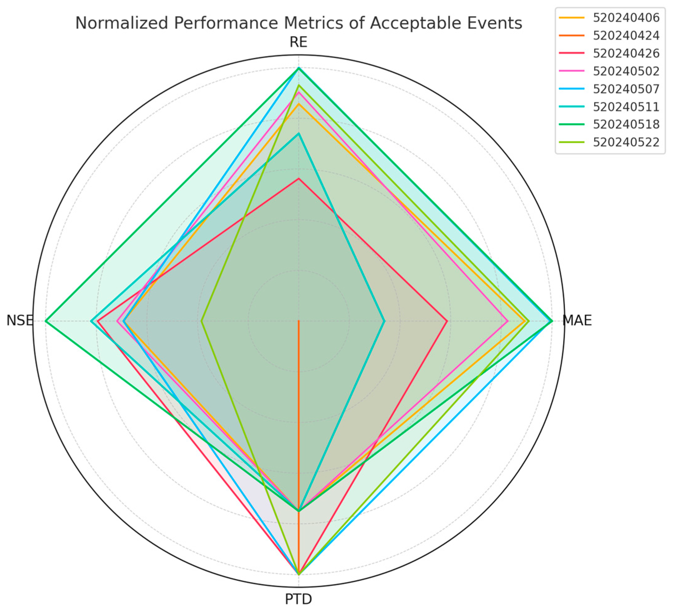
To substantiate the representativeness of this event and avoid concerns of overfitting, a normalized radar chart analysis was performed across all qualified calibration events. The evaluation included multiple criteria, and for the error-related metrics, reverse normalization was applied to ensure a consistent interpretation, with higher values representing better performance. As shown in Figure 5, event 520240518 exhibited balanced and high-ranking performance across all metrics. Though other events occasionally outperformed in individual dimensions, none achieved such consistent quality overall.

In addition to its numerical superiority, event 520240518 exhibited hydrological features, including moderate rainfall, a single-peak hydrograph, and clear response dynamics, all of which support parameter stability. Given its balanced performance across multiple criteria and favorable runoff dynamics, this event was chosen as the calibration benchmark.

4.2. Simulation Results and Model Applicability Assessment

4.2.1. Simulation Results

This study evaluated the flood forecasting performance of the Xin’anjiang model using four flood events as independent validation cases. These include three typical flood events observed in 2024 (event IDs: 520240531, 520240613, and 520240818), as well as an extreme flood event recorded on 7 June 2020 (denoted as event 20200607), which corresponds to a 50-year return period.

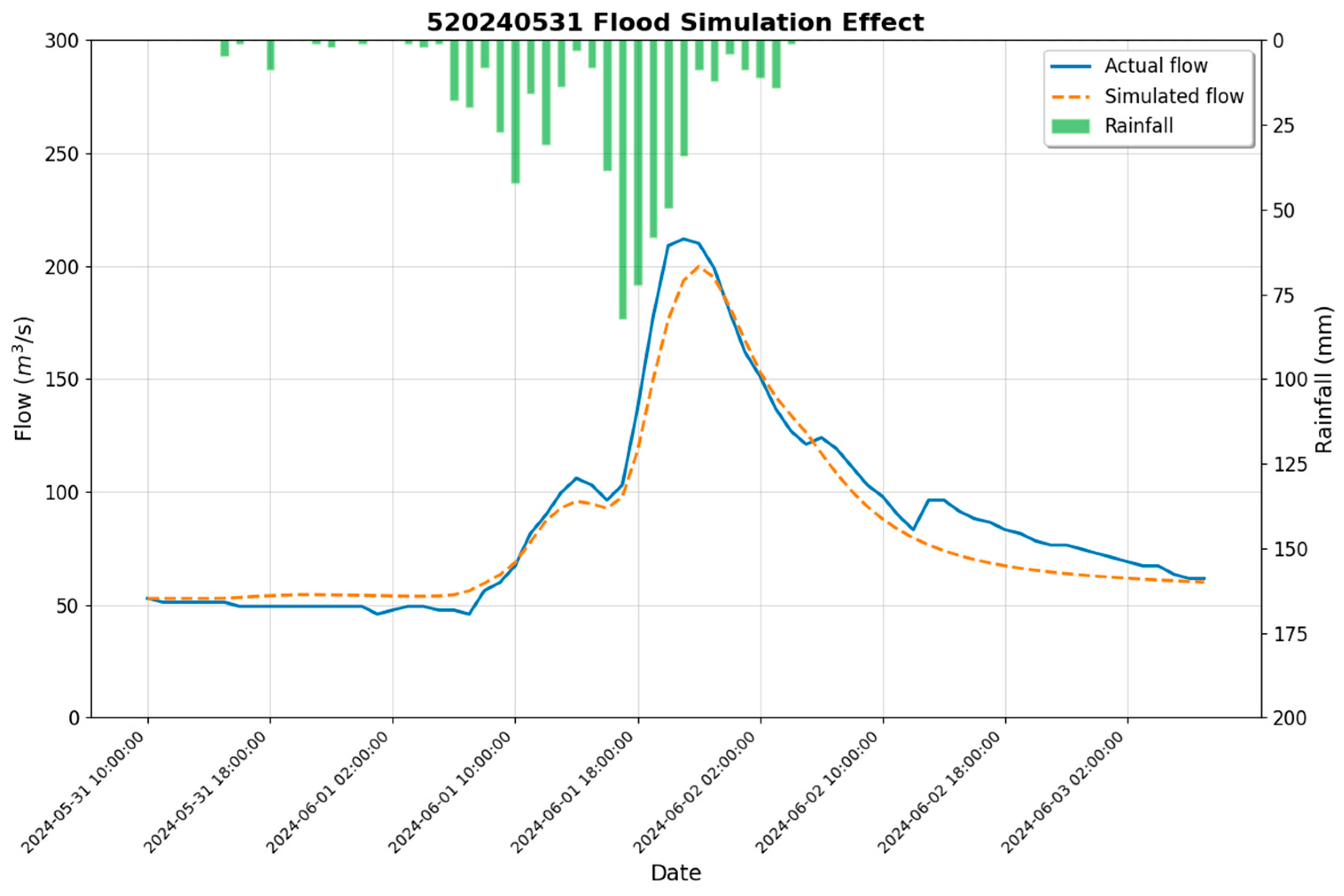
The rainfall runoff simulation results for each event are illustrated in Figure 6, Figure 7, Figure 8 and Figure 9. Specifically, the performance for flood events 520240531, 520240613, and 520240818 are shown in Figure 6, Figure 7 and Figure 8, respectively, while the simulation of the extreme flood in 2020 is presented in Figure 9. These cases were selected to represent a range of hydrometeorological conditions and test the model’s applicability to both typical and high-magnitude flood scenarios.

4.2.2. Applicability Assessment

During flood event 520240531, the simulated discharge process exhibited general consistency with the observed hydrograph in the overall trend. The model effectively captured the watershed’s flow variation characteristics during most periods. The simulation results accurately reflected both the timing and variation trend of flood peaks. During the rising limb following increased rainfall, the model demonstrated satisfactory reproduction of the runoff response processes. A clear correlation was observed between the rainfall variation and subsequent simulated discharge changes, with simulated peak discharges closely approximating observed values (NSE = 0.9469). This indicates that the parameter calibration process adequately accounted for hydrological hysteresis effects. Although minor deviations were observed in specific time intervals, particularly slight underestimations of peak magnitudes or temporal shifts (±0.5–1.2 h) in peak timing, the overall simulation error remained within acceptable limits. The superior model performance metrics confirm that the SCE-UA algorithm-calibrated parameters possess high precision and applicability for this flood simulation scenario.

During flood event 520240613, the simulated discharge process generally aligned with the observed hydrograph in the overall trend. The model effectively captured the flow variations induced by multiple rainfall peaks, demonstrating high sensitivity and adaptability to complex rainfall events. The simulated flood peaks were slightly higher than the observed values in some periods, and the recession limb of the simulated hydrograph appeared steeper than that which was observed. This discrepancy may primarily stem from the model’s assumption of uniform rainfall distribution across the watershed, whereas actual rainfall exhibited spatial differences, potentially amplifying the localized hydrological responses. The parameters that were calibrated by the SCE-UA algorithm achieved satisfactory performance in simulating multi-peak flood events, with accurate prediction of flood peak timing.

During flood event 520240818, the simulated discharge values closely matched the observed data in the initial phase (e.g., from midnight to early morning on August 18) under light and scattered rainfall conditions, demonstrating the model’s reliable response capability to low-intensity precipitation. As the rainfall intensified, particularly during the morning to noon period on August 18, when precipitation reached its peak, the simulated discharge values progressively increased and successfully captured the variation trend of the flow. Although minor deviations existed, the simulation exhibited good overall consistency with the observations, indicating robust predictive performance under heavy rainfall conditions.

During the rainfall recession and flow recession phase (from the afternoon of August 18 to the early morning of the following day), the simulated discharge values gradually declined in agreement with the observed trend. However, discrepancies between the simulated and observed values emerged during the recession phase, likely attributable to complex factors such as soil infiltration and groundwater interactions.

The NSE coefficient for the entire simulation period reached 0.9565, confirming the model’s strong overall performance in discharge calculations throughout this flood event.

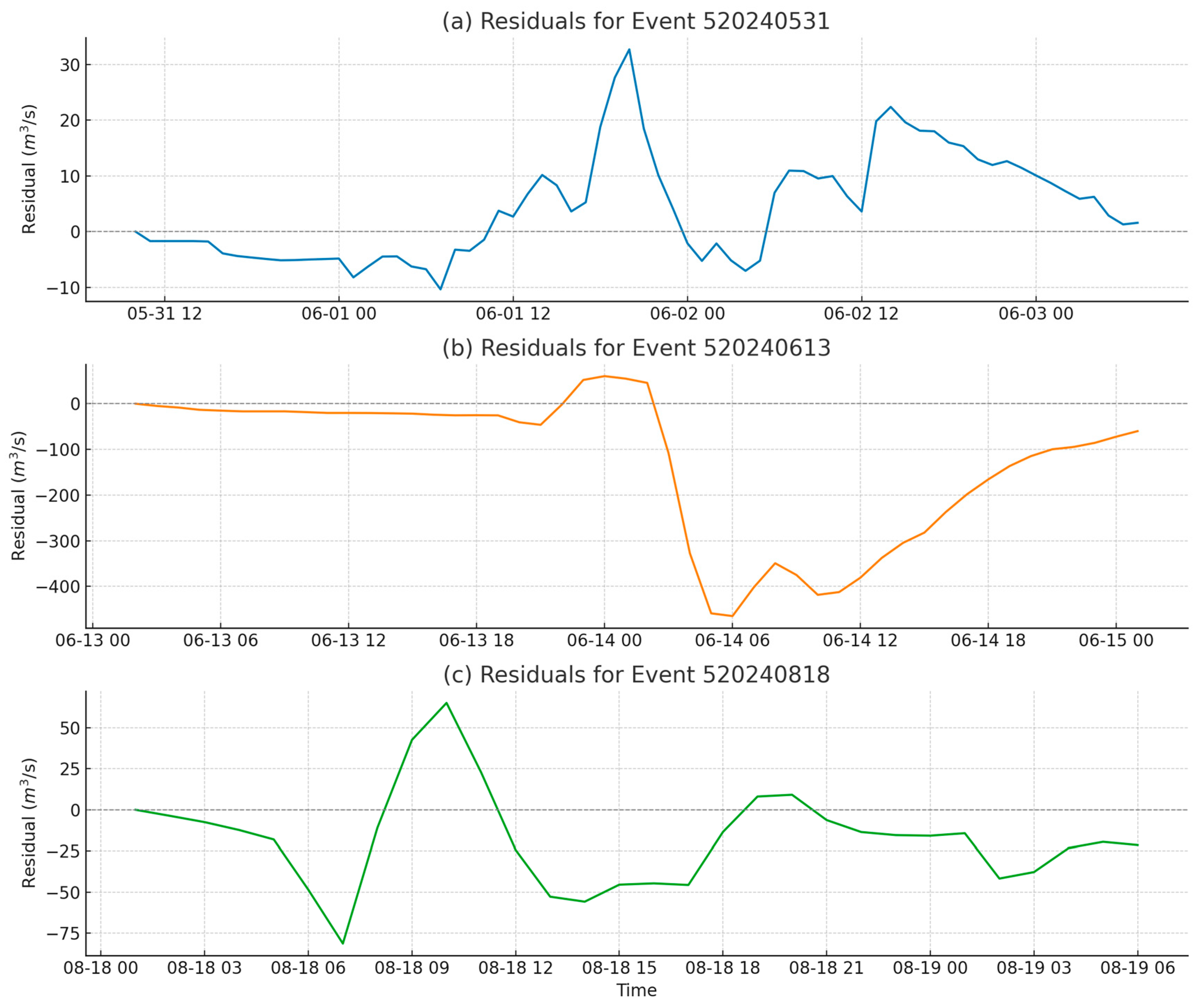
To further evaluate the discrepancies between the observed and simulated flows, residual plots for the three validation events were produced (Figure 10). The residuals generally oscillate around zero, indicating no systematic bias in the model outputs. For event 520240531 and event 520240613, the residuals during rising and falling limbs remain within ±50 m³/s, reflecting good overall consistency. Slight underestimations were observed during the recession phase of event 520240818, which is consistent with the previously discussed hydrograph analysis. These patterns confirm that the model captures the temporal structure of flood processes reasonably well.

To extend the model validation beyond typical flood scenarios, this study further simulates the extreme flood event that occurred on 7 June 2020 in the Pa River basin. This event was induced by a rapidly developing frontal system and southwest monsoonal inflow, generating over 370 mm of rainfall at Damiaoxia Station within seven hours. The areal average precipitation upstream reached 211.8 mm, and the observed peak discharge at Damiaoxia was 1750 m³/s. Historical records indicate that this event corresponds to an approximate 50-year return period flood, featuring a rapid runoff concentration and steep hydrograph rise [45].

Using the previously calibrated Xin’anjiang model parameter set, the simulation reproduced key hydrological characteristics of the event. As shown in Figure 9, the simulated hydrograph matched the observed rising limb and flood peak timing with high consistency. The simulated peak discharge reached approximately 1523 m³/s, resulting in a relative error of −12.97%, and the Nash–Sutcliffe Efficiency (NSE) reached 0.86. A minor underestimation was observed during the falling limb, which is likely due to the model’s simplified treatment of recession processes. In particular, the recession curve in the Xin’anjiang framework is jointly controlled by the baseflow coefficient and soil moisture thresholds, which are less responsive to the delayed drainage caused by deep saturation and antecedent moisture accumulation. Furthermore, the lumped formulation neglects spatial variability in rainfall intensity, which likely played a role during this event, where rainfall in select sub-catchments exceeded 350 mm while other zones received considerably less.

The overall alignment of peak timing, magnitude, and hydrograph morphology suggests that the calibrated Xin’anjiang model retains predictive effectiveness under extreme rainfall runoff conditions. The simulation captures the essential process of saturation-excess runoff generation and its rapid translation into flood peaks within the short time window characteristic of flash-flood-prone regions like the Pa River basin.

The analysis demonstrates that the Xin’anjiang model—when calibrated with the SCE-UA algorithm—exhibits competent predictive capabilities for extreme rainfall events, though further refinement of its recession phase simulation accuracy remains necessary. Subsequent research should consider incorporating refined surface water–groundwater coupling parameters to enhance prediction reliability under complex hydrological conditions.

Despite varying rainfall patterns across the four flood events, the calibrated model manifested strong adaptability in both single-peak and multi-peak flood scenarios. Specifically, the model successfully replicated the complete flood hydrograph (peak magnitude and recession process) during the single-peak event 520240531 while accurately capturing dynamic variations between successive flood peaks in the multi-peak event 520240613. These results confirm that the SCE-UA-optimized Xin’anjiang model can efficiently and accurately simulate diverse flood processes in the Pa River basin.

While this study focuses on automated optimization through the SCE-UA algorithm, it is worth noting that conventional manual calibration approaches or single-parameter sensitivity tuning have long been employed in hydrological practice. Compared to such traditional methods, the proposed event-wise global calibration strategy enables a more consistent and reproducible parameter identification process, especially under complex multi-storm and extreme event conditions. Future work could consider benchmarking the Xin’anjiang model against empirical or statistical models to further evaluate its comparative advantages under different catchment characteristics.

4.3. Parameter Sensitivity Analysis

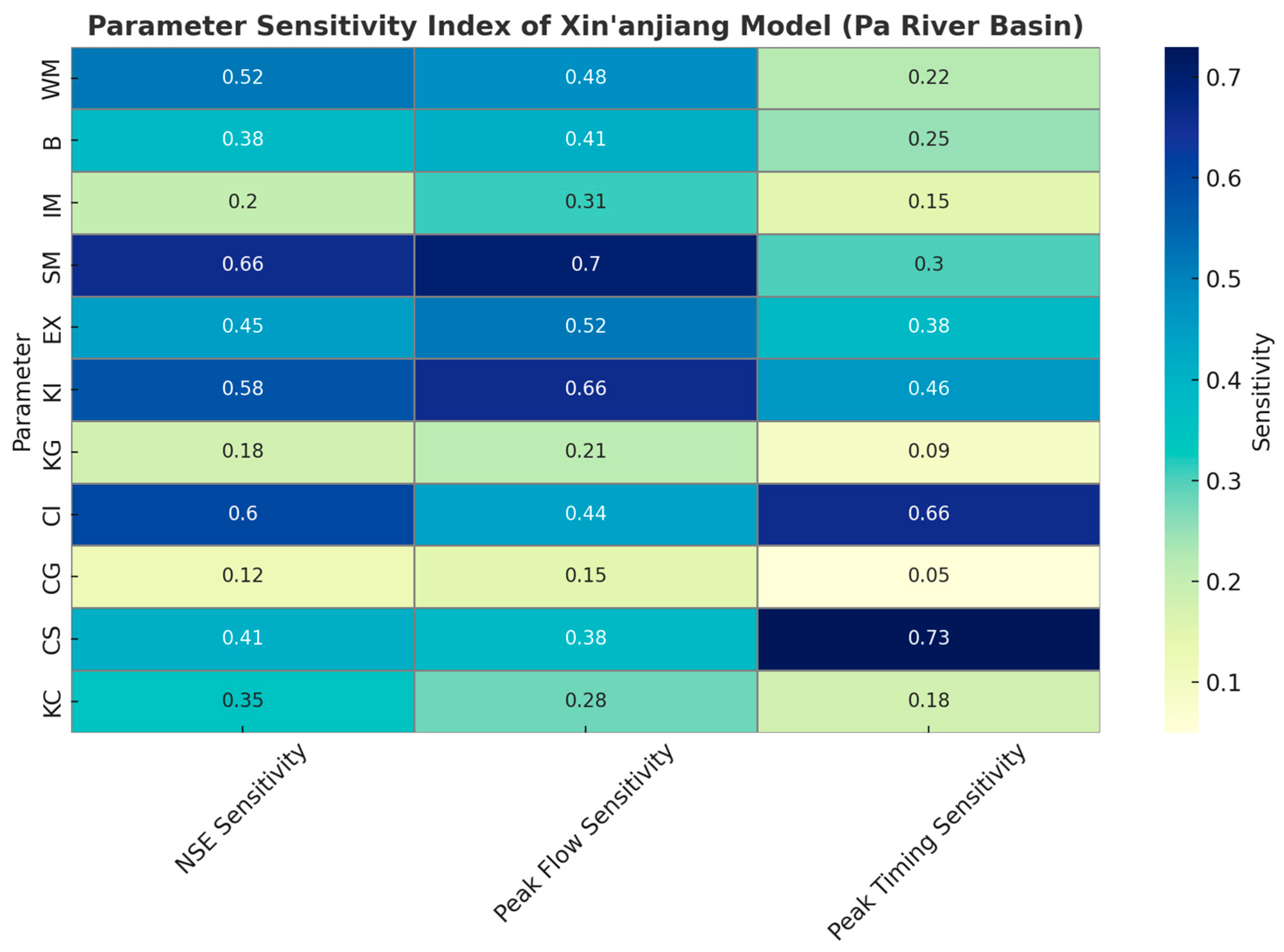
To better understand the response behavior of the Xin’anjiang model under flood-prone conditions in the Pa River basin, a quantitative sensitivity assessment was conducted on the eleven calibrated parameters. The analysis focused on three key evaluation metrics: Nash–Sutcliffe Efficiency (NSE), peak discharge (Qp), and Peak Timing Deviation (PTD). A one-at-a-time perturbation approach was employed, whereby each parameter was individually adjusted by ±10% around its calibrated value while the remaining parameters were held constant. The resulting deviations in the model outputs were averaged across the twelve calibration events to derive normalized sensitivity indices.

The results are summarized in

Table 5. Sensitivity index of calibrated parameters.

Parameter	NSE Sensitivity	Peak Flow Sensitivity	Peak Timing Sensitivity
WM	0.52	0.48	0.22
B	0.38	0.41	0.25
IM	0.20	0.31	0.15
SM	0.66	0.70	0.30
EX	0.45	0.52	0.38
KI	0.58	0.66	0.46
KG	0.18	0.21	0.09
CI	0.60	0.44	0.66
CG	0.12	0.15	0.05
CS	0.41	0.38	0.73
KC	0.35	0.28	0.18

and visualized in Figure 11. The parameters exerting the greatest influence on model performance were those associated with rapid runoff generation and routing. Notably, free water storage capacity (SM) and the interflow coefficient (KI) exhibited consistently high sensitivity across all metrics. These parameters govern the production and timing of near-surface flow, which is the dominant runoff mechanism in this steep-sloped and shallow soil watershed.

The interflow recession constant (CI) also demonstrated high responsiveness, particularly in peak timing, due to its role in shaping the recession limb of the hydrograph. For example, the slightly accelerated recession observed in events such as 520240613 and 520240818 is likely related to the relatively high sensitivity of CI and CS. Conversely, parameters associated with slower hydrological processes, such as groundwater recession (CG) and deep storage (KG), displayed limited sensitivity, which aligns with their marginal influence during short-duration, high-intensity flood events. Similarly, the evapotranspiration adjustment factor (KC) had a minor effect, as expected, given the brief temporal scale of the analyzed storms.

Event-specific performance further supports the interpretation of parameter impacts. For instance, in the simulation of the June 2020 extreme flood, an accurate reproduction of the peak discharge and rising limb suggests that SM and KI were effectively tuned to capture the rapid storm response. On the other hand, in mid-intensity floods such as event 520240518, model performance remained stable with lower reliance on the high-sensitivity routing parameters.

The distribution of sensitivities reinforces the physical realism of the model configuration. Though the sensitivity indices provide a representative average across events, their specific influence may vary due to the differences in rainfall spatial structure, antecedent soil moisture, and event duration.

This sensitivity analysis contributes to a clearer understanding of how individual parameters affect model performance under different hydrological conditions. Parameters such as WM (tension water capacity) and KI (interflow runoff coefficient) exhibit relatively higher standardized sensitivity coefficients, suggesting a stronger influence on runoff generation processes in the Pa River basin. This result aligns with the dominant hydrological behaviors observed in humid subtropical catchments, where rapid saturation and lateral flow are key contributors during rainfall events.

This analysis helps highlight the parameters that are more responsive to changes in model outputs, which may inform future calibration strategies or observational priorities in similar environments. Furthermore, examining sensitivity across multiple calibration events provides some indication of parameter consistency, thereby adding a degree of confidence to the model’s transferability across events of varying magnitude and temporal structure.

Incorporating sensitivity diagnostics alongside standard performance metrics also enhances the interpretability of model behavior, offering a complementary perspective that supports a more process-oriented understanding of the Xin’anjiang model’s functioning in flood simulation tasks.

5. Conclusions

This study developed a flood forecasting framework for the Pa River basin by calibrating the key parameters of the Xin’anjiang model using the SCE-UA global optimization algorithm. A total of 16 measured flood events were analyzed, among which 12 were used for parameter calibration and 4 for independent validation—including a 50-year return period extreme flood that occurred in June 2020.

The calibrated model demonstrated strong consistency in reproducing flood peak timing, magnitude, and overall runoff processes. Across the validation events, the Nash–Sutcliffe Efficiency (NSE) values exceeded 0.85, relative errors in peak discharge were generally within ±10%, and peak timing deviations were limited to 1–3 h. The quantitative sensitivity analysis further identified WM, B, and SM as the most influential parameters affecting simulation accuracy.

While this study focuses on physically based modeling with global parameter calibration, future work could benefit from benchmarking the Xin’anjiang model against data-driven or distributed hydrological models such as SWAT, HEC-HMS, or machine learning approaches. Such comparisons would help position the current methodology within a broader modeling context and highlight its advantages and limitations under different data availability and basin conditions. One current limitation is the absence of quantitative uncertainty analysis. Future studies could incorporate Monte Carlo simulations or Bayesian inference to quantify the confidence bounds of model outputs. This would provide more robust insights into forecast reliability under parameter and rainfall variability [46].

These results confirm that the SCE-UA-enhanced Xin’anjiang model is capable of simulating both typical and extreme flood events in the Pa River basin under current climatic conditions. While the model has not yet been applied to real-time forecasting operations, the established workflow provides a feasible basis for future forecasting applications and flood risk management in data-limited basins. Further improvements should involve long-term, multi-year calibration and enhanced spatial rainfall monitoring to improve model adaptability to complex hydrometeorological regimes. These insights suggest that the framework, although tested in a regional context, could be extended to similar flood-prone catchments globally, particularly under monsoonal or subtropical regimes.

References

1. Fornarelli, R.; Galelli, S.; Castelletti, A.; Antenucci, J.P.; Marti, C.L. An Empirical Modeling Approach to Predict and Understand Phytoplankton Dynamics in a Reservoir Affected by Interbasin Water Transfers. Water Resour. Res. 2013, 49, 3626–3641. [Google Scholar] [CrossRef]
2. Ewen, J.; O’Connell, E.; Bathurst, J.; Birkinshaw, S.J.; Kilsby, C.; Parkin, G.; O’Donnell, G. Physically-Based Modelling, Uncertainty, and Pragmatism Comment on: ‘Systeme Hydrologique Europeen (She): Review and Perspectives After 30 Years Development in Distributed Physically-Based Hydrological Modelling’ by Jens Christian Refsgaard, Borge Storm and Thomas Clausen. Hydrol. Res. 2012, 43, 945–947. [Google Scholar] [CrossRef]
3. Beven, K. Towards an Alternative Blueprint for a Physically Based Digitally Simulated Hydrologic Response Modelling System. Hydrol. Process. 2002, 16, 189–206. [Google Scholar] [CrossRef]
4. Efstratiadis, A.; Koutsoyiannis, D. One Decade of Multi-Objective Calibration Approaches in Hydrological Modelling: A Review. Hydrol. Sci. J. 2010, 55, 58–78. [Google Scholar] [CrossRef]
5. Zhang, L.; Meng, X.; Wang, H.; Yang, M.; Cai, S. Investigate the Applicability of CMADS and CFSR Reanalysis in Northeast China. Water 2020, 12, 996. [Google Scholar] [CrossRef]
6. Reichstein, M.; Camps-Valls, G.; Stevens, B.; Jung, M.; Denzler, J.; Carvalhais, N.; Prabhat. Deep Learning and Process Understanding for Data-Driven Earth System Science. Nature 2019, 566, 195–204. [Google Scholar] [CrossRef]
7. Chen, E.; Andersen, M.S.; Chandra, R. Deep Learning Framework with Bayesian Data Imputation for Modelling and Forecasting Groundwater Levels. Environ. Model. Softw. 2024, 178, 106072. [Google Scholar] [CrossRef]
8. Vrugt, J.A. Distribution-Based Model Evaluation and Diagnostics: Elicitability, Propriety, and Scoring Rules for Hydrograph Functionals. Water Resour. Res. 2024, 60, e2023WR036710. [Google Scholar] [CrossRef]
9. Mix, K.; Lopes, V.L.; Rast, W. A Systems Approach to Understanding the Evolution of the Agro-Social-Ecological System of the Upper Rio Grande-San Luis Valley, Colorado. Water Resour. Manag. 2015, 29, 233–251. [Google Scholar] [CrossRef]
10. Seong, C.; Her, Y.; Benham, B.L. Automatic Calibration Tool for Hydrologic Simulation Program-FORTRAN Using a Shuffled Complex Evolution Algorithm. Water 2015, 7, 503–527. [Google Scholar] [CrossRef]
11. Naeini, M.R.; Analui, B.; Gupta, H.V.; Duan, Q.; Sorooshian, S. Three Decades of the Shuffled Complex Evolution (SCE-UA) Optimization Algorithm: Review and Applications. Sci. Iran. 2019, 26, 2015–2031. [Google Scholar]
12. Vrugt, J.A.; Gupta, H.V.; Bastidas, L.A.; Bouten, W.; Sorooshian, S. Effective and Efficient Algorithm for Multiobjective Optimization of Hydrologic Models. Water Resour. Res. 2003, 39. [Google Scholar] [CrossRef]
13. Lee, S.; Kang, T. Analysis of Constrained Optimization Problems by the SCE-UA with an Adaptive Penalty Function. J. Comput. Civ. Eng. 2016, 30, 04015035. [Google Scholar] [CrossRef]
14. Xu, Y.; Liu, C.; Yu, Q.; Zhao, C.; Quan, L.; Hu, C. Study on a Hybrid Hydrological Forecasting Model SCE-GUH by Coupling SCE-UA Optimization Algorithm and General Unit Hydrograph. Water 2023, 15, 2783. [Google Scholar] [CrossRef]
15. Wang, Z.; Zhang, X.; Liu, C.; Ren, L.; Cai, X.; Li, K. Hydrological Simulation and Parameter Optimization Based on the Distributed Xin’anjiang Model and the Particle Swarm Optimization Algorithm: A Case Study of Xunhe Watershed in Shandong, China. Water 2024, 16, 3168. [Google Scholar] [CrossRef]
16. Huang, S.; Zhang, L.; Li, D. Research on Simpliffied Evaluation Method for Soil-Rock Mixed Slope Stability Under Dam-Break Flood Impact. Bull. Eng. Geol. Environ. 2025, 84, 46. [Google Scholar] [CrossRef]
17. Xu, H.; Zhao, Y.; Dajun, Z.; Duan, Y.; Xu, X. Exploring the Typhoon Intensity Forecasting Through Integrating AI Weather Forecasting with Regional Numerical Weather Model. NPJ Clim. Atmos. Sci. 2025, 8, 38. [Google Scholar] [CrossRef]
18. Ikeuchi, K.; Kakinuma, D.; Nakamura, Y.; Numata, S.; Mochizuki, T.; Kubota, K.; Yasukawa, M.; Nemoto, T.; Koike, T. Development of Flash Flood Forecasting System for Small and Medium-Sized Rivers. J. Flood Risk Manag. 2025, 18, e70026. [Google Scholar] [CrossRef]
19. Wu, M.; Gao, Y.; Liu, Y.; Xu, L.; Gao, L. Application and Effect Evaluation of Different Optimization Algorithms in Distributed Hydrological Model. J. Hydrol. Reg. Stud. 2025, 58, 102207. [Google Scholar] [CrossRef]
20. Kan, G.; He, X.; Ding, L.; Li, J.; Liang, K.; Hong, Y. A Heterogeneous Computing Accelerated SCE-UA Global Optimization Method Using OpenMP, OpenCL, CUDA, and OpenACC. Water Sci. Technol. 2017, 76, 1640–1651. [Google Scholar] [CrossRef]
21. Kan, G.; Liang, K.; Li, J.; Ding, L.; He, X.; Hu, Y.; Amo-Boateng, M. Accelerating the SCE-UA Global Optimization Method Based on Multi-Core CPU and Many-Core GPU. Adv. Meteorol. 2016, 2016, 8483728. [Google Scholar] [CrossRef]
22. Borga, M.; Anagnostou, E.N.; Bloeschl, G.; Creutin, J.D. Flash Flood Forecasting, Warning and Risk Management: The Hydrate Project. Environ. Sci. Policy 2011, 14, 834–844. [Google Scholar] [CrossRef]
23. Dore, J.; Lebel, L.; Molle, F. A Framework for Analysing Transboundary Water Governance Complexes, Illustrated in the Mekong Region. J. Hydrol. 2012, 466, 23–36. [Google Scholar] [CrossRef]
24. Yuan, F.; Ren, L.-L.; Yu, Z.-B.; Xu, J. Computation of Potential Evapotranspiration Using a Two-Source Method for the Xin’anjiang Hydrological Model. J. Hydrol. Eng. 2008, 13, 305–316. [Google Scholar] [CrossRef]
25. Zhang, M.; Wang, J.; Huang, Y.; Yu, L.; Liu, S.; Ma, G. A New Xin’anjiang and Sacramento Combined Rainfall-Runoff Model and Its Application. Hydrol. Res. 2021, 52, 1173–1183. [Google Scholar] [CrossRef]
26. Jahanshahi, A.; Booij, M.J.; Patil, S.D. Dependence of Rainfall-Runoff Model Performance on Calibration Conditions Under Changing Climatic Conditions. Hydrol. Sci. J. 2025, 70, 581–596. [Google Scholar] [CrossRef]
27. Xu, C.; Zhong, P.-a.; Zhu, F.; Xu, B.; Wang, Y.; Yang, L.; Wang, S.; Xu, S. A Hybrid Model Coupling Process-Driven and Data-Driven Models for Improved Real-Time Flood Forecasting. J. Hydrol. 2024, 638, 131494. [Google Scholar] [CrossRef]
28. Wang, A.; Pianosi, F.; Wagener, T. Technical Report-Methods: A Diagnostic Approach to Analyze the Direction of Change in Model Outputs Based on Global Variations in the Model Inputs. Water Resour. Res. 2020, 56, e2020WR027153. [Google Scholar] [CrossRef]
29. Syvitski, J.P.M.; Vörösmarty, C.J.; Kettner, A.J.; Green, P. Impact of Humans on the Flux of Terrestrial Sediment to the Global Coastal Ocean. Science 2005, 308, 376–380. [Google Scholar] [CrossRef]
30. Walling, D.E. Human Impact on Land-Ocean Sediment Transfer by the World’s Rivers. Geomorphology 2006, 79, 192–216. [Google Scholar] [CrossRef]
31. Cheng, Y.; Sang, Y.; Wang, Z.; Guo, Y.; Tang, Y. Effects of Rainfall and Underlying Surface on Flood Recession-The Upper Huaihe River Basin Case. Int. J. Disaster Risk Sci. 2021, 12, 111–120. [Google Scholar] [CrossRef]
32. Fischer, S.; Buehler, P.; Schumann, A. Impact of Flood Types on Superposition of Flood Waves and Flood Statistics Downstream. J. Hydrol. Eng. 2021, 26, 04021024. [Google Scholar] [CrossRef]
33. Ashok, K.; Saji, N.H. On the Impacts of ENSO and Indian Ocean Dipole Events on Sub-Regional Indian Summer Monsoon Rainfall. Nat. Hazards 2007, 42, 273–285. [Google Scholar] [CrossRef]
34. Zhou, T.J.; Yu, R.C. Atmospheric Water Vapor Transport Associated with Typical Anomalous Summer Rainfall Patterns in China. J. Geophys. Res. Atmos. 2005, 110. [Google Scholar] [CrossRef]
35. Jin, D.; Guan, Z.; Huo, L.; Wang, X. Possible Impacts of Spring Sea Surface Temperature Anomalies over South Indian Ocean on Summer Rainfall in Guangdong-Guangxi Region of China. Clim. Dyn. 2017, 49, 3075–3090. [Google Scholar] [CrossRef]
36. Ding, Y.H.; Chan, J.C.L. The East Asian Summer Monsoon: An Overview. Meteorol. Atmos. Phys. 2005, 89, 117–142. [Google Scholar] [CrossRef]
37. Schutte, C.; van der Laan, M.; van der Merwe, B. Leveraging Historic Streamflow and Weather Data with Deep Learning for Enhanced Streamflow Predictions. J. Hydroinform. 2024, 26, 835–852. [Google Scholar] [CrossRef]
38. GB/T 22482-2008; Standard for Hydrological Information and Hydrological Forecasting. China Standards Press: Beijing, China, 2008.
39. Paradis, D.; Gloaguen, E.; Lefebvre, R.; Giroux, B. A Field Proof-of-Concept of Tomographic Slug Tests in an Anisotropic Littoral Aquifer. J. Hydrol. 2016, 536, 61–73. [Google Scholar] [CrossRef]
40. Ronen-Eliraz, G.; Ginat, H.; Dody, A.; Blumberg, D.; Dahan, O. Flood Hydrograph Reconstruction from the Peak Flow Value in Ephemeral Streams Using a Simplified Robust Single-Parameter Model. Hydrol. Process. 2016, 30, 3004–3013. [Google Scholar] [CrossRef]
41. Anwar, H.; Khan, A.U.; Ullah, B.; Taha, A.T.B.; Najeh, T.; Badshah, M.U.; Ghanim, A.A.J.; Irfan, M. Intercomparison of Deep Learning Models in Predicting Streamflow Patterns: Insight from CMIP6. Sci. Rep. 2024, 14, 17468. [Google Scholar] [CrossRef]
42. Fischer, S.; Schumann, A.; Buehler, P. Timescale-Based Flood Typing to Estimate Temporal Changes in Flood Frequencies. Hydrol. Sci. J. 2019, 64, 1867–1892. [Google Scholar] [CrossRef]
43. Jeon, J.-H.; Park, C.-G.; Engel, B.A. Comparison of Performance Between Genetic Algorithm and SCE-UA for Calibration of SCS-CN Surface Runoff Simulation. Water 2014, 6, 3433–3456. [Google Scholar] [CrossRef]
44. Wang, Z.; Xu, N.; Bao, X.; Wu, J.; Cui, X. Spatio-Temporal Deep Learning Model for Accurate Streamflow Prediction with Multi-source Data Fusion. Environ. Model. Softw. 2024, 178, 106091. [Google Scholar] [CrossRef]
45. He, J.B. Analysis of the “2020.6 Extreme Storm Flood in the Panjiang River”. Water Resour. Sci. Cold Zone Eng. 2022, 5, 63–65. [Google Scholar]
46. Yang, J.; Wen, L.; Guo, J.; Chen, Y.; Zhu, Y.; Wang, Y.; Ma, M. A Cooperative Search Algorithm-Based Flood Forecasting Framework: Application Across Diverse Chinese Catchments. Front. Earth Sci. 2025, 13, 1538235. [Google Scholar] [CrossRef]
Figure 1. Workflow of Xin’anjiang model setup and parameter calibration using the SCE-UA algorithm.
Water 17 01154 g001
Figure 2. Architectural flowchart of the Xin’anjiang hydrological model.
Water 17 01154 g002
Figure 3. SCE optimization algorithm flowchart.
Water 17 01154 g003
Figure 4. Spatial distribution of hydrometric stations and hydrographic system schematic in the Shuitou Town Reach of the Pa River basin.
Water 17 01154 g004
Figure 5. Radar chart comparing normalized performance metrics of selected calibration events.
Water 17 01154 g005
Figure 6. Simulation hydrograph for flood event 520240531.
Water 17 01154 g006
Figure 7. Simulation hydrograph for flood event 520240613.
Water 17 01154 g007
Figure 8. Simulation hydrograph for flood event 520240818.
Water 17 01154 g008
Figure 9. Simulation hydrograph for extreme flood event 20200607.
Water 17 01154 g009
Figure 10. Residuals between observed and simulated discharges for validation events: (a) event 520240531, (b) event 520240613, and (c) event 520240818.
Water 17 01154 g010
Figure 11. Sensitivity heatmap of Xin’anjiang model parameters with respect to NSE, peak discharge, and peak timing across 12 calibration events.
Water 17 01154 g011