Study on the Temporal Variability and Influencing Factors of Baseflow in High-Latitude Cold Region Rivers: A Case Study of the Upper Emuer River

Abstract

Baseflow is a crucial component of river flow in alpine inland basins, playing an essential role in watershed ecological health and water resource management. In high-latitude cold regions, seasonal freeze-thaw processes make baseflow formation mechanisms particularly complex. However, the dominant factors affecting baseflow and their relative contributions remain unclear, limiting the accuracy of flow estimation and effective water resource management. This study employed baseflow separation techniques and statistical methods, including the Mann-Kendall test, to investigate temporal trends and abrupt changes in baseflow and the baseflow index (BFI) at multiple time scales (annual, seasonal, and monthly) from 2005 to 2012. Additionally, the timing of snowmelt and its impact on baseflow were examined. Key findings include the following: (1) Baseflow and BFI showed distinct temporal variability with non-significant upward trends across all time scales. Annual BFI ranged from 0.48 to 0.61, contributing approximately 50% of total runoff. (2) At the seasonal scale, baseflow remained relatively stable in spring, increased in autumn, and showed non-significant decreases in summer and winter. Monthly baseflow exhibited an increasing trend. (3) The snowmelt period occurred between April and May, with baseflow during this period strongly correlated with climatic factors in the following order: winter precipitation > positive accumulated temperature > winter air temperature > negative accumulated temperature. The strongest positive correlation was observed between baseflow and winter precipitation (R = 0.724), while negative correlations were found with accumulated temperatures and winter air temperature. These findings offer valuable insights for predicting water resource availability and managing flood and ice-jam risks in cold regions.

1. Introduction

Cold regions are essential components of global ecosystems, characterized by their unique climatic and hydrological processes [1,2]. In China, cold regions cover approximately 4.17 × 10⁶ km², accounting for about 43.5% of the country’s total land area [3]. Permafrost and seasonally frozen soil are widely distributed across these regions, forming a complex groundwater system influenced by various hydrological and geological conditions. Precipitation in high-latitude cold regions primarily occurs as snowfall during winter, which accumulates on the surface and subsequently melts in spring, serving as a major source of runoff [4]. The concentrated melting of snow and ice during this period often leads to a rapid increase in surface runoff over a short duration, potentially causing hazards such as ice jams, ice dams, and ice floods [5,6]. In contrast to rivers in non-cold regions, cold region rivers exhibit distinct seasonal variations in runoff. Annual runoff in these regions presents periodic changes, with the flood season (wet period) typically accounting for more than 70% of the total annual runoff, while the non-flood season (low-flow period) contributes less than 30%. During the freezing period (dry season), runoff is even lower, sometimes constituting less than 1% of the annual total [7]. Baseflow plays a critical role in maintaining river flow during periods of low precipitation and minimal surface runoff, especially during the winter when snow is accumulated or in early spring following seasonal snowmelt. During this time, when rainfall is scarce, direct runoff mainly comprises surface runoff and subsurface flow generated by snowmelt, making baseflow a key contributor to river flow [8]. Therefore, understanding baseflow dynamics in cold region is essential for evaluating groundwater–surface water interactions across different seasons, improving spring flood forecasting, and enhancing disaster prevention and mitigation measures [9,10].

Cold region rivers are highly sensitive to climate change, with their seasonal variations directly affecting the sustainable management of water resources [1,11]. Numerous studies have examined the dynamic changes in cold region runoff and projected future trends through various methodologies [12,13,14], including hydrological observations [15], isotope methods [16], and model simulations [17,18]. These studies have shown that runoff variations in cold region rivers are influenced not only by climatic factors, such as precipitation and temperature [19], but also by other factors like frozen soil degradation [20,21], land use changes [22], and snowmelt processes [23]. For instance, Yang et al. [24] emphasized the significance of interactions between climate conditions and land use changes in driving runoff variations within cold region watersheds. Additionally, Connon et al. [25] demonstrated how disruptions in the freeze-thaw cycle could alter snowmelt runoff recharge pathways, thereby affecting runoff composition in permafrost degradation areas. Recent advancements in data-driven technologies, including the integration of remote sensing and model simulation techniques, have provided powerful tools for assessing the spatiotemporal variability and future trends of runoff in large-scale cold region watersheds [26,27]. For example, the use of GRACE satellite data has enabled the quantification of changes in water storage within permafrost regions, revealing their potential impacts on the hydrological cycle [28,29]. However, most studies have concentrated on overall runoff characteristics, and research specifically focusing on baseflow dynamics in high-latitude cold regions remains limited. Furthermore, the mechanisms underlying baseflow variations and their sensitivity to climatic factors remain unclear. In recent years, studies on baseflow in cold regions have been limited, and the patterns of change and underlying mechanisms of baseflow in these regions remain unclear.

The study of baseflow is complicated by the diverse factors influencing its behavior, including topography, natural environment, hydrological elements, soil type, and regional geology, which affect the applicability of various baseflow separation methods [30,31,32]. Researchers have applied various methods to investigate baseflow dynamics and their evolutionary patterns. Commonly used techniques include graphical methods, automatic segmentation numerical simulations, hydrological models, and isotope-based methods [33]. Ramli et al. [34] employed the Chapman baseflow separation method to estimate baseflow contributions in the Peusangan Basin. Zhang et al. [35] applied the baseflow index method, HYSEP, and digital filtering to analyze baseflow characteristics and future trends in the middle reaches of the Yellow River. Additionally, Bosch et al. [36] found that baseflow proportions are higher during dry years, highlighting the importance of accurate baseflow estimation during drought conditions. Eckhardt [37] compared multiple baseflow separation methods and concluded that the two-parameter filter method offers more stable and reliable baseflow hydrographs, making it suitable for analyzing hydrological processes across various time steps and watershed characteristics.

Despite these advances, research on baseflow in cold region rivers, particularly in high-latitude areas of China, is still insufficient. Few studies have systematically examined baseflow trends, variability, and influencing factors in these regions. While some studies have applied isotope methods to distinguish baseflow sources and estimate the contributions of snowmelt runoff, glacial meltwater, and groundwater [38,39], these methods have limitations when applied to large-scale, high-latitude basins. Moreover, although machine learning and other advanced data-driven approaches have shown potential in hydrological modeling and baseflow estimation, their application to cold region rivers is still in its infancy [40,41].

The Emuer River, located in the remote cold region area of China, offers a unique opportunity to investigate baseflow characteristics in high-latitude environment. However, most existing research focuses on general river flow characteristics, with limited attention given to baseflow analysis. To address this gap, the present study employs hydrometeorological data from the Emuer River Basin spanning the period 2005–2012, applying the digital filtering method to separate baseflow and analyzed baseflow index (BFI) trends and abrupt changes across various temporal scales. Furthermore, the study investigated the relationship between baseflow and climatic factors during the snowmelt period. The findings of this study provide a theoretical basis for the effective and sustainable management of water resources in cold regions, offering valuable insights for water resource allocation and disaster risk management under changing climate conditions.

2. Materials and Methods

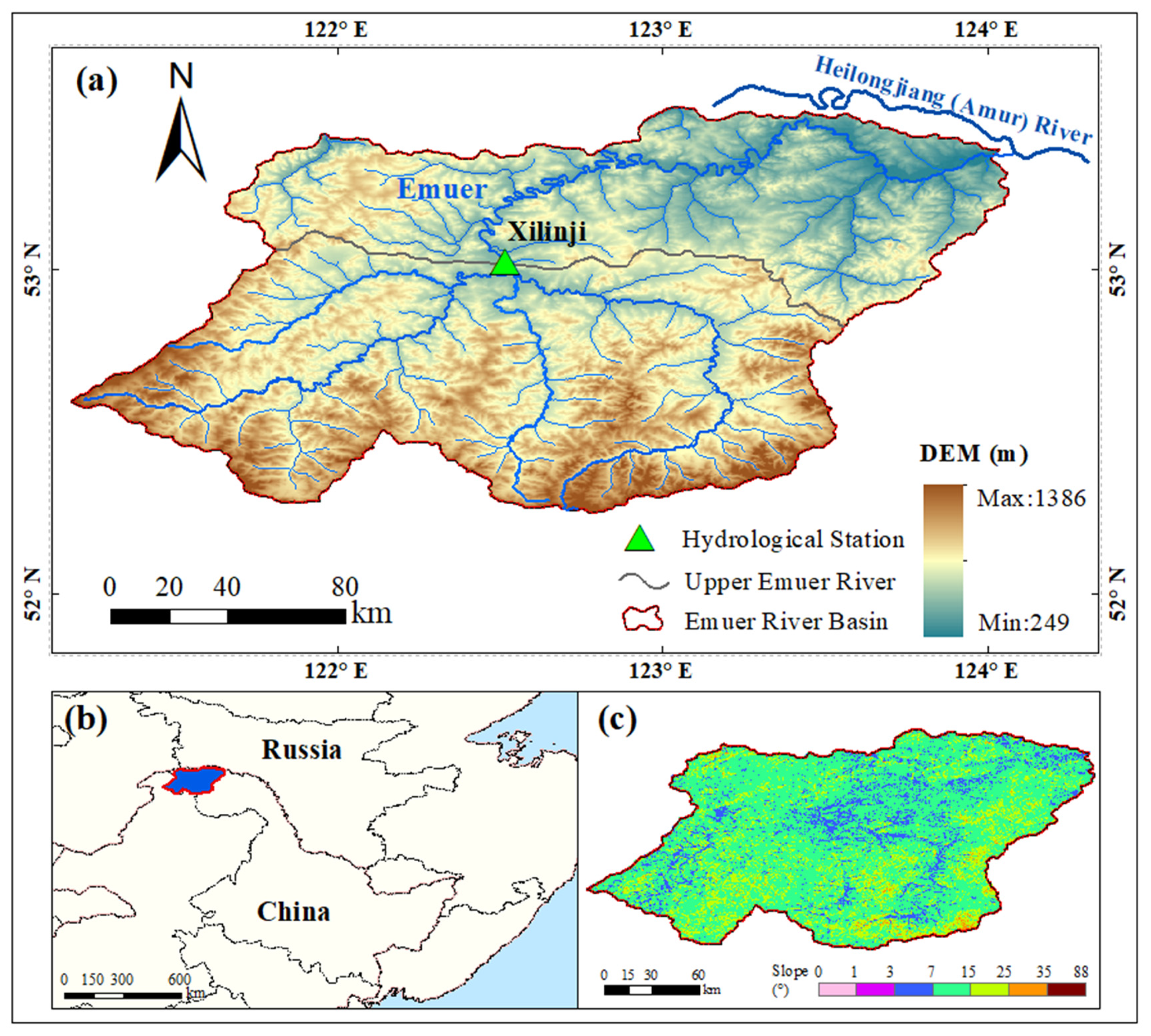
2.1. Study Area

The Emuer River is a right-bank tributary of the international border river, the Heilongjiang (Amur) River, located in Mohe City of Heilongjiang Province, China. The basin covers an area of 16,280 km², with widespread permafrost distribution throughout the region. The climate is classified as cold temperate continental monsoon, with an annual average temperature of −5.5 °C and annual precipitation of 460.8 mm, of which about 262.44 mm occurs in summer (June to August), while only 12.93 mm occurs in winter (December to February) [42]. The long-term average discharge is 86.5 m³/s, with an annual streamflow of 2.73 × 10⁸ m³, and the annual average runoff depth is 149.61 mm [43]. Precipitation is mainly concentrated in the summer months of July and August, accounting for approximately 75% of the annual total, which often leads to summer flooding. Spring runoff primarily arises from snowmelt due to rising temperatures, with snowmelt runoff and ice jams contributing to severe ice flood events. In winter, the river freezes due to low temperatures, and runoff is predominantly supported by baseflow [44]. Consequently, analyzing the temporal characteristics of baseflow is critical for effective water resource management and flood prevention in the basin.

The Xilinji Hydrological Station is located in the upper reaches of the Emuer River. The geographical location, elevation, and slope distribution of the basin, along with the hydrological observation station, are shown in Figure 1. The Emuer River originates from the Zhi Jichang Mountain in the Greater Khingan Range and flows northward, collecting tributaries such as the Lao Cao River, Gu Lian River, and Da Lin River, before joining the Heilongjiang (Amur) River near Xing’an Township in the northeast. The southern portion of the basin is characterized by the hilly terrain of the Greater Khingan Range, with an average elevation of approximately 1000 m, while the northern and central areas are dominated by plains at an elevation of 600 m. The overall slope of the basin is relatively gentle, with slopes predominantly in the range from 3° to 7° and from 7° to 15° (Figure 1c). From a geological perspective, the Emuer River Basin is located in the Mohe Basin in the Northeast of China, at the tectonic boundary between the Siberian and Northeast China blocks [45]. The basin’s geology is primarily composed of fine gravel, gravelly sandstone, fine sandstone, and silty mudstone [46].

2.2. Data Source

Meteorological data from 2005 to 2012 were obtained from the National Meteorological Information Center of the China Meteorological Administration (http://data.cma.cn/en, accessed on 27 October 2024), including key variables such as temperature and precipitation. Hydrological data for the same period, consisting of daily runoff records for the Upper Emuer River Basin, were collected from the Xilinji Hydrological Station in Mohe City. The hydrology data were primarily used to analyze the temporal variability of baseflow, while precipitation and temperature data were employed to assess their influence on baseflow. Before the analysis, all datasets underwent quality control, with missing data filled using a 5-day moving average method. Digital Elevation Model (DEM) data were sourced from the Geospatial Data Cloud platform (http://hfbfh0c9ce6dccd2e4eefs6fo005xx0vko6bcw.fgac.hlju.cwkeji.cn/, accessed on 15 October 2024), specifically using the SRTM DEM dataset with a spatial resolution of 90 m. DEM imagery covering Northeast China was selected, and the DEM data for the study area were prepared by merging and clipping these images using ArcMap 10.6 software.

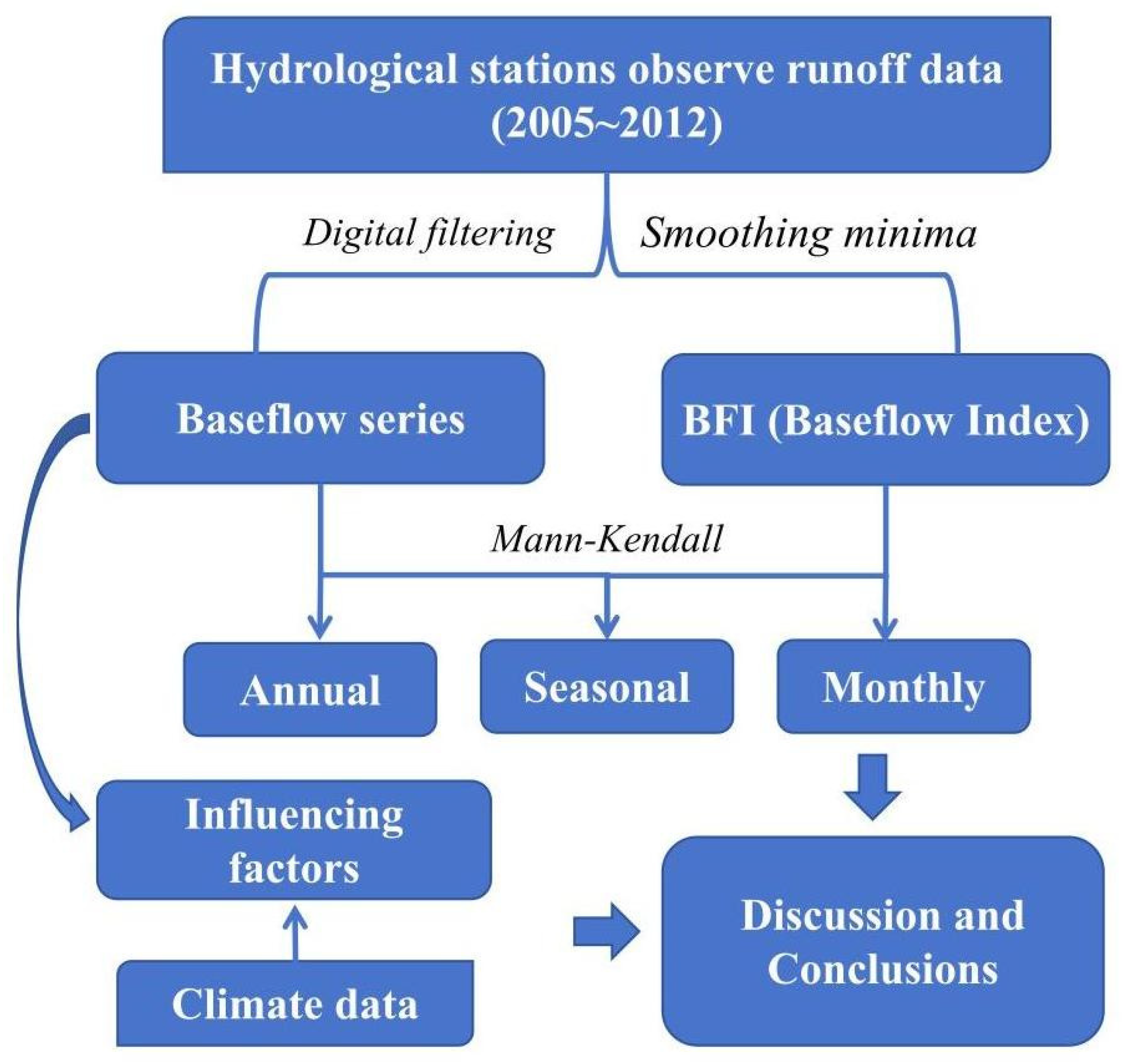
2.3. Methods

The flowchart of the study is shown in Figure 2. First, the baseflow and baseflow index (BFI) for the Upper Emuer River Basin from 2005 to 2012 are calculated using the digital filtering method and the smoothing minima method, respectively. Then, the evolution patterns at the annual, seasonal, and monthly scales are analyzed. Finally, the influencing factors of baseflow during the snowmelt period are examined.

2.3.1. Digital Filtering Method

The digital filtering method, originally developed for digital signal processing, was first introduced as the Lyne-Hollick filter in 1979 [47]. Nathan and McMahon (1990) adapted this method for baseflow estimation [48]. In 2005, Eckhardt refined the method by proposing a recursive digital filtering method, which enhanced baseflow estimation accuracy and produced smoother baseflow hydrographs. This study employs the recursive digital filtering method to partition baseflow and analyzed its temporal evolution. The formula for this method is as follows:

$$q_{b\left(i\right)}={\displaystyle \frac{\alpha \left(1-{BFI}_{max}\right)q_{b\left(i-1\right)}+\left(1-\alpha \right){BFI}_{max}{q}_{\left(i\right)}}{1-\alpha {BFI}_{max}}}$$

(1)

In the formula, α is typically set to 0.95. ${BFI}_{max}$ represents the maximum, which is used to describe the proportion of baseflow that is maximized in the total streamflow, and typically varies as an empirical value under different conditions. Eckhardt proposed the value of ${BFI}_{max}$ for different hydrogeological conditions to eliminate the subjective influence brought by the calculation process. Eckhardt pointed out that for perennial rivers with porous and transmissive aquifers (characterized by high porosity and transmissivity), ${BFI}_{max}$ is typically 0.80, whereas for seasonal rivers, it is 0.50. Perennial streams with fractured hard rock aquifers have a ${BFI}_{max}$ value of 0.25. In order to make the segmentation of the baseflow more accurate, ${BFI}_{max}$ can be selected as the maximum of the baseflow ratio of the smoothing minima method [37].

2.3.2. Smoothing Minima Method

The smoothing minima method was first proposed by the UK Institute of Hydrology in 1980 [49]. Based on variations in the turning point test factor, the method can be categorized into the standard smoothing minima method and its improved version. In this study, the standard smoothing minima method is employed, with $\mathrm{f}=0.9$. The choice of $\mathrm{f}=0.9$ is based on previous studies that have demonstrated its effectiveness in capturing baseflow patterns while minimizing the interference of short-term runoff fluctuations. This parameter value is commonly applied in hydrological studies focusing on low-flow analysis and baseflow separation, providing a balance between sensitivity and stability in the detection of turning points. The principle involves dividing the daily runoff series into $365/N$ units and selecting the minimum value from each unit. These minima form a hydrological series $q_1,q_2,q_3,\cdots ,q_m$. The sequence is then segmented as $\left(q_1,q_2,q_3\right),\left(q_2,q_3,q_4\right),\cdots ,\left(q_{t-1},q_t,q_{t+1}\right)$. If the turning point factor $\mathrm{f}{\mathrm{q}}_{\mathrm{t}}\le \mathrm{m}\mathrm{i}\mathrm{n}\left(q_{t-1},q_{t+1}\right)$, $q_t$ is identified as a turning point. The turning point condition does not explicitly include $q_t$ in the comparison, but it is valid as the turning point is determined by comparing the current value $q_t$ with the neighboring values $q_{t-1}$ and $q_{t+1}$. All turning points are determined using this method, and the baseflow values for other times are obtained through linear interpolation. The total baseflow volume is then calculated as the area under the baseflow hydrograph [50]. In this study, the smoothing minima method is used to calculate the BFI and analyze its temporal evolution. $N$ refers to the number of units into which the daily runoff series is divided, and for the purpose of this study, $t$ is the time index in days, applied on a daily time scale [44,45].

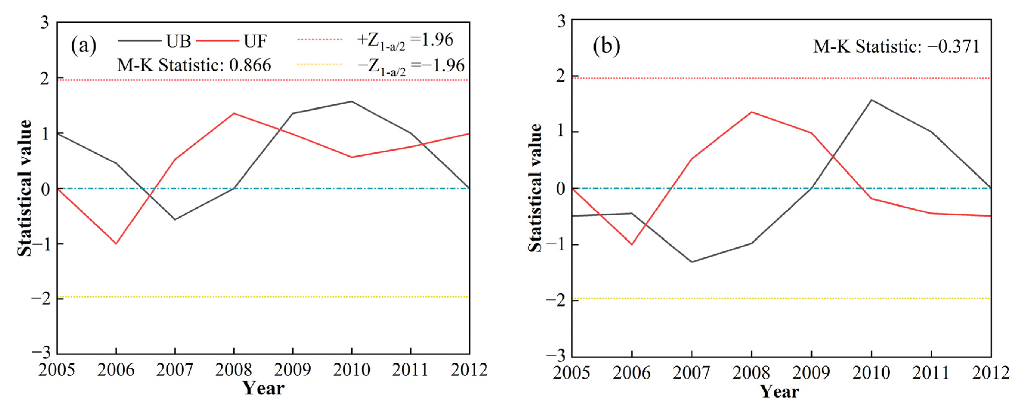
2.3.3. Mann-Kendall Non-Parametric Test

The Mann-Kendall test is a non-parametric statistical method recommended by the World Meteorological Organization (WMO) [51] and has been widely applied to analyze temporal trends in runoff and meteorological factors in recent years [52]. In this study, the Mann-Kendall trend test implemented in MATLAB R2018a is used to examine the trends and abrupt changes in baseflow across different temporal scales [53].

The specific formula is as follows [54,55]:

$$\mathrm{s}\mathrm{g}\mathrm{n}({\mathrm{x}}_{\mathrm{j}}-{\mathrm{x}}_{\mathrm{i}})=\left\{\begin{array}{c}1\\ 0\\ -1\end{array}\begin{array}{c}\mathrm{i}\mathrm{f} {\mathrm{x}}_{\mathrm{j}}>{\mathrm{x}}_{\mathrm{i}}\\ \mathrm{i}\mathrm{f} {\mathrm{x}}_{\mathrm{j}}={\mathrm{x}}_{\mathrm{i}}\\ \mathrm{i}\mathrm{f} {\mathrm{x}}_{\mathrm{j}}<{\mathrm{x}}_{\mathrm{i}}\end{array}\right.$$

(2)

$$\mathrm{S}={\sum }_{\mathrm{i}=1}^{\mathrm{n}-1}{\sum }_{\mathrm{j}=\mathrm{i}+1}^{\mathrm{n}}\mathrm{s}\mathrm{g}\mathrm{n}({\mathrm{x}}_{\mathrm{j}}-{\mathrm{x}}_{\mathrm{i}})$$

(3)

where $\mathrm{s}\mathrm{g}\mathrm{n}({\mathrm{x}}_{\mathrm{j}}-{\mathrm{x}}_{\mathrm{i}})$ is the sign function, ${\mathrm{x}}_{\mathrm{i}}$ and ${\mathrm{x}}_{\mathrm{j}}$ are the values in time series $\mathrm{i}$ and $\mathrm{j}$ ($\mathrm{j}>\mathrm{i}$), respectively, and $\mathrm{n}$ denotes the total number of observations in the time series. The variance is calculated as follows:

$$\mathrm{V}\mathrm{a}\mathrm{r}(\mathrm{S})={\displaystyle \frac{\mathrm{m}(\mathrm{m}-1)(2\mathrm{m}+5)-{\sum }_{\mathrm{i}=1}^{\mathrm{p}}{\mathrm{t}}_{\mathrm{i}}({\mathrm{t}}_{\mathrm{i}}-1)(2{\mathrm{t}}_{\mathrm{i}}+5)}{18}}$$

(4)

where $\mathrm{m}$ is the number of tied groups, $\mathrm{p}$ is the number of fixed groups, and ${\mathrm{t}}_{\mathrm{i}}$ denoted the number of relationships in the number $\mathrm{i}$ range. A fixed group (also called a tied group) refers to a set of data points in the time series that share the same value. These tied observations affect the variance of the Mann-Kendall test statistic; therefore, a correction term is applied to account for their influence. For each tied group $\mathrm{i}$, its size ${\mathrm{t}}_{\mathrm{i}}$ is included in the variance formula to adjust for tied ranks. When $\mathrm{m}$ is greater than 10, the Mann-Kendall statistical value ${\mathbf{Z}}_{\mathbf{M}\mathbf{K}}$ can be calculated using the following formula:

$${\mathrm{Z}}_{\mathrm{M}\mathrm{K}}=\left\{\begin{array}{c}{\displaystyle \frac{\mathrm{S}-1}{\sqrt{\mathrm{v}\mathrm{a}\mathrm{r}\left(\mathrm{S}\right)}}}S>0\\ 0S=0\\ {\displaystyle \frac{\mathrm{S}+1}{\sqrt{\mathrm{v}\mathrm{a}\mathrm{r}\left(\mathrm{S}\right)}}}S<0\end{array}\right.$$

(5)

At a specified significance level $\mathsf{\alpha }$, if $\left|{\mathbf{Z}}_{\mathbf{M}\mathbf{K}}\right|>{\mathbf{Z}}_{\mathbf{1}-\mathsf{\alpha }/\mathbf{2}}$, the null hypothesis of no trend is rejected, indicating a significant trend in the time series data. ${\mathbf{Z}}_{\mathbf{1}-\mathsf{\alpha }/\mathbf{2}}$ represents the value corresponding to the standard normal distribution table at a given confidence level $\mathsf{\alpha }$. Specifically, when the absolute value of ${\mathbf{Z}}_{\mathbf{M}\mathbf{K}}$ exceeds 1.6, 1.96, and 2.58, it signifies that the trend has passed the significance tests at confidence levels of 90%, 95%, and 99%, respectively [56].

2.3.4. Pearson Correlation Coefficient

The Pearson correlation coefficient is a statistical method used to assess the strength and direction of the linear relationship between two variables. It is commonly applied to evaluate correlations between datasets to determine whether they align on a straight line. In this study, the Pearson correlation coefficient is used to quantify the correlation between baseflow and meteorological factors. The formula is as follows:

$$\mathbf{r}={\displaystyle \frac{{\sum }_{\mathbf{i}}^{\mathbf{n}}\left({\mathbf{X}}_{\mathbf{i}}-\overline{\mathbf{X}}\right)\left({\mathbf{Y}}_{\mathbf{i}}-\overline{\mathbf{Y}}\right)}{\sqrt{{\sum }_{\mathbf{i}}^{\mathbf{n}}{\left({\mathbf{X}}_{\mathbf{i}}-\overline{\mathbf{X}}\right)}^{\mathbf{2}}{\sum }_{\mathbf{i}}^{\mathbf{n}}{\left({\mathbf{Y}}_{\mathbf{i}}-\overline{\mathbf{Y}}\right)}^{\mathbf{2}}}}}$$

(6)

In the formula, $\mathbf{r}$ represents the correlation coefficient, which ranges from −1 to 1. When $\mathbf{r}\mathbf{>}\mathbf{0}$, it indicates a positive correlation; when $\mathbf{r}\mathbf{<}\mathbf{0}$, it indicates a negative correlation; and when $\mathbf{r}\mathbf{=}\mathbf{0}$, it indicates no correlation. ${\mathbf{X}}_{\mathbf{i}}$ and ${\mathbf{Y}}_{\mathbf{i}}$ represent the values of the two variables in the sample, while $\overline{\mathbf{X}}$ and $\overline{\mathbf{Y}}$ represent the mean values of the two variables [57].

3. Results and Analysis

3.1. Temporal Variations in Baseflow

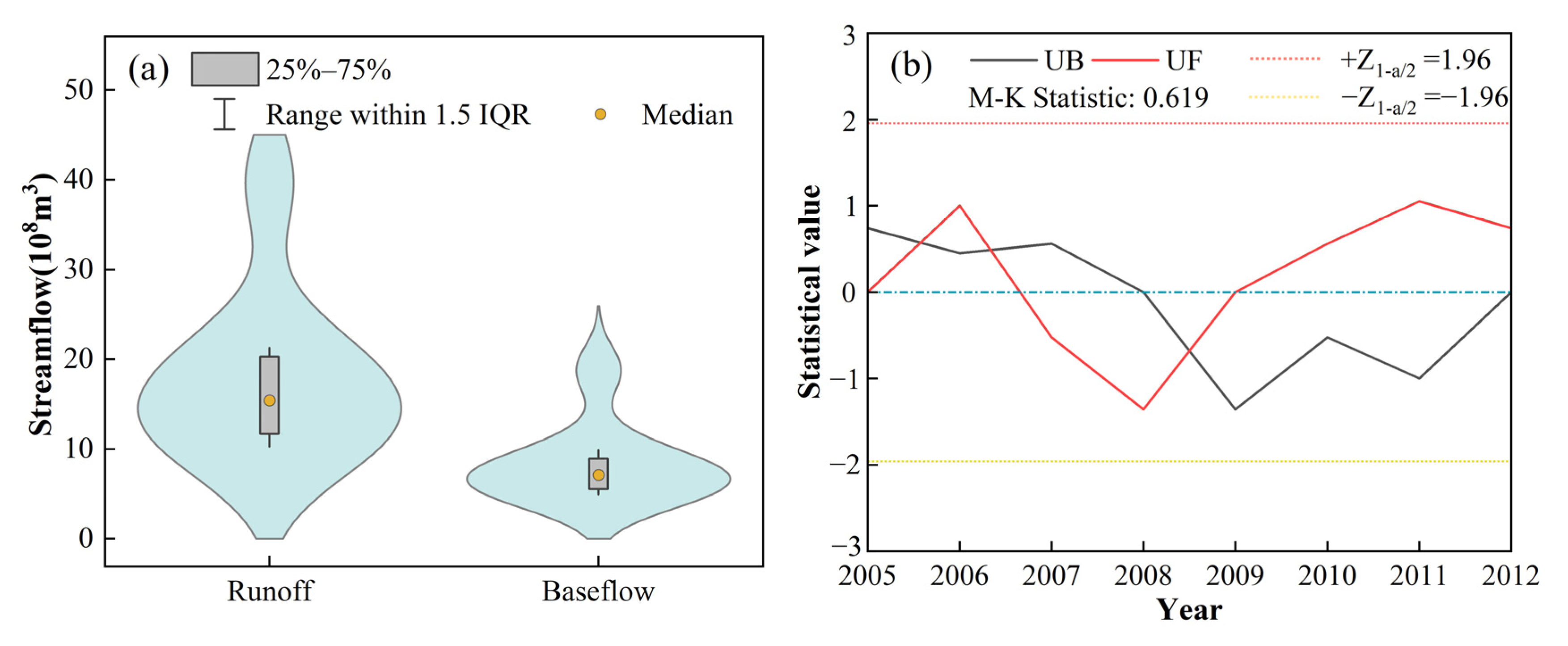
3.1.1. Analysis of Annual Scale Evolution Patterns

Using daily runoff measurements from the Xilinji Hydrological Station in the Upper Emuer River Basin, the ECK recursive digital filtering method was applied to separate the baseflow from the observed river discharge data spanning from 2005 to 2012. By incorporating violin plots into the boxplot-based statistical analysis, the violin plot effectively illustrates the statistical characteristics of the data. The violin plot represents the density distribution of values within a given range, with the shape on both sides reflecting the distribution pattern. The median indicates the central tendency of the data, while the box represents the interquartile range (IQR), spanning from the 25th to the 75th percentile, which reflects the degree of data dispersion. The variations in runoff and baseflow are presented in Figure 3a. Both annual runoff and baseflow exhibit relatively consistent distribution patterns, following a normal distribution. The median line in the boxplot highlights the central tendency, and the noticeable difference between the medians of runoff and baseflow suggests significant disparities in their central tendencies. Compared to annual runoff, the interquartile range of baseflow is narrower, indicating less dispersion and a more concentrated distribution, while annual runoff demonstrates greater variability. Statistical analysis indicates that the annual baseflow generally ranges from 4.92 to 18.79 × 10⁸ m³, with the lowest baseflow in 2008 and the highest in 2009. The multi-year average baseflow is 8.35 × 10⁸ m³. From 2005 to 2012, annual baseflow exhibited a stable upward trend, consistent with the overall runoff trend, with a coefficient of variation of 0.5, indicating a high interannual variability of baseflow. The trend in runoff change was more pronounced than that of baseflow. The growth rates of baseflow and runoff were 0.43 × 10⁸ m³/year and 0.72 × 10⁸ m³/year, respectively. As runoff increased, the proportion of baseflow in total river discharge also increased.

To further examine trends and detect abrupt changes in baseflow, the Mann-Kendall (M-K) trend test was applied to the baseflow time series. As shown in Figure 3b, the ${\mathbf{Z}}_{\mathbf{M}\mathbf{K}}$ was 0.619, which did not pass the 95% significance level, indicating no statistically significant increasing trend. The UF and UB statistical curves intersect near 2006 and 2008, with their intersection points lying within the threshold of ±1.96 [54,55], suggesting that baseflow underwent notable changes around 2006 and 2008.

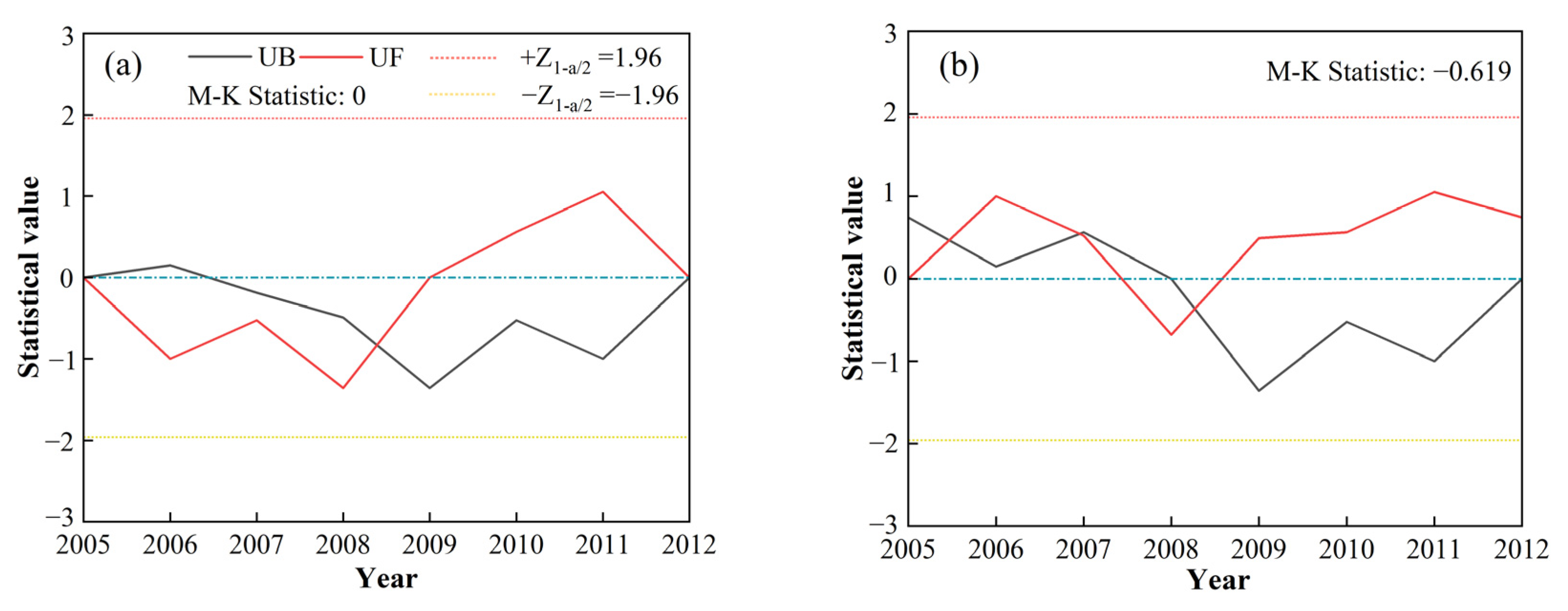
3.1.2. Analysis of Seasonal Scale Evolution Patterns

The seasonal baseflow of the Emuer River was calculated and is presented in Figure 4. Spring, autumn, and winter exhibited a normal distribution, while summer showed a skewed distribution. The interquartile range, reflecting data dispersion, indicates that variability ranks as summer > spring > autumn, suggesting that autumn baseflow is the most concentrated and stable, while summer baseflow shows the highest variability and significant fluctuations. Median comparisons reveal that the summer median is significantly higher than those of spring and autumn, indicating a more pronounced trend during summer. Seasonal baseflow distribution varies considerably, with average baseflows of 1.45 × 10⁸ m³ in spring, 4.37 × 10⁸ m³ in summer, 2.51 × 10⁸ m³ in autumn, and 0.01 × 10⁸ m³ in winter. The Upper Emuer River experiences substantial inter-annual runoff fluctuations, with low-flow periods typically occurring during spring and winter. In winter, low temperatures cause precipitation to accumulate as snow and the river to freeze, resulting in a sharp decline in runoff. Conversely, at the end of spring, rising temperatures and precipitation cause snowmelt, leading to a rapid increase in runoff. Consequently, seasonal baseflow is most abundant in summer and autumn, exhibiting a wider range of variation, while spring and winter baseflows are narrower and more stable, consistent with general runoff patterns. An analysis of the coefficients of variation (Cv) for baseflow across the four seasons from 2005 to 2012 reveals Cv values of 0.48 for spring, 0.59 for summer, 0.48 for autumn, and 1.00 for winter. The variability of summer baseflow was relatively high, with a right-skewed violin plot and the widest interquartile range (IQR). This suggests that the highest variability occurs during winter, which is likely due to the limited flow conditions.

The Mann-Kendall (M-K) trend analysis and mutation point detection were performed for the seasonal baseflow of spring, summer, autumn, and winter from 2005 to 2012, as shown in Figure 5a–d. The ${\mathbf{Z}}_{\mathbf{M}\mathbf{K}}$ for baseflow trends in spring, summer, autumn, and winter were 0, −0.619, 1.361, and −0.124, respectively. The seasonal baseflow growth rates, in descending order, are summer > autumn > spring > winter. The M-K mutation test detected mutations in 2008 for spring; 2005, 2007, and 2008 for summer; 2008 and 2010 for autumn; and 2011 for winter. Notably, the spring, summer, and autumn seasons all experienced mutations in 2008. The observed fluctuations in seasonal baseflow suggest considerable variability, which likely results from the diverse hydrological systems and unique environmental conditions of high-latitude cold regions, thereby contributing to mutations that occur across multiple seasons and years.

3.1.3. Analysis of Monthly Scale Evolution Patterns

Between 2005 and 2012, the mean monthly streamflow from May to October ranged from 1.60 to 3.12 × 10⁸ m³, indicating higher flow values, with the wet season predominantly occurring during these months. The multi-year average monthly baseflow peaked at 1.29 × 10⁸ m³ in August, while the minimum value of 0 was recorded during winter. The study area is characterized by extensive seasonally frozen soil, with riverbed freezing commonly occurring in winter. Meteorological and hydrological data reveal that from December to March, the Emuer River experiences persistent flow cessation due to subzero temperatures, resulting in no observable baseflow variation from January to March. Baseflow begins to emerge in April as temperatures rise and snowmelt commences. Monthly baseflow in the Upper Emuer River exhibits significant intra-annual variation, as illustrated in Figure 6. April, July, and September exhibited a consistent distribution pattern, characterized by skewed distributions, while the remaining months followed a roughly normal distribution. A clear trend is evident in the median lines of the boxplots, with August showing a significantly higher median compared to April. Furthermore, August displays the widest interquartile range, indicating higher dispersion and pronounced variability. During the study period, the monthly baseflow predominantly ranged between 0 and 5 × 10⁸ m³. The coefficient of variation (Cv) for monthly baseflow varied from 1.89 in April to 0.13 in September, highlighting greater dispersion in April and August. The most substantial and smallest ranges of baseflow variation were observed in August and the winter months of January, February, and March, respectively.

The temporal variation of the baseflow is influenced by local climatic and hydrological factors, particularly temperature, precipitation, and snowmelt. In spring (April–May), rising temperatures trigger snowmelt, enhancing baseflow as meltwater recharges groundwater. The high Cv value in April reflects variability in snowmelt timing and intensity, which depends on winter precipitation and temperature. In summer (June–August), increased precipitation boosts groundwater recharge, with peak baseflow in August resulting from cumulative rainfall and gradual groundwater release. The low Cv value in September indicates a stable baseflow pattern supported by sustained groundwater contributions. During autumn (September–October), baseflow declines as precipitation decreases and recharge is limited, but delayed discharge from the wet season maintains river flow. In winter (November–March), freezing temperatures inhibit recharge and riverbed freezing restricts flow, leading to minimal baseflow variation from January to March.

The Mann-Kendall trend analysis and corresponding statistical results for monthly baseflow from April to December are presented in

Table 1. Mann-Kendall test of interannual monthly baseflow.

Month	${\mathbf{Z}}_{\mathbf{M}\mathbf{K}}$	Trend	Significance Test
April	0.86603	Increase	Non-Significant
May	0.12372	Increase	Non-Significant
June	−0.12372	Decrease	Non-Significant
July	0.37115	Increase	Non-Significant
August	0.61859	Increase	Non-Significant
September	1.6083	Increase	Significant
October	0.86603	Increase	Non-Significant
November	−0.61859	Decrease	Non-Significant
December	−0.12372	Decrease	Non-Significant

. The interannual variability of baseflow exhibited an increasing trend in April, May, and from July to October, with the variation in September demonstrating statistical significance at the 90% confidence level. Conversely, a decreasing trend in interannual variability was observed in June, November, and December. Through M-K mutation detection, irregular patterns of baseflow variation were identified across months and years, with noticeable fluctuation at mutation points. Specifically, the mutation year for April was 2006, while May experienced a mutation in 2008. June and July exhibited mutations in 2007 and 2009, respectively. Mutations for August, September, and October all occurred in 2008. November experienced mutations in 2006 and 2007, while December’s mutation year was identified as 2011. In summary, the monthly and annual variations in baseflow are complex and irregular, lacking clear periodicity or consistency. The observed BFI changes across different months are mainly driven by snowmelt, precipitation patterns, temperature fluctuations, and the region’s distinct hydrological characteristics, including seasonally frozen soil and riverbed freezing processes.

3.2. Temporal Variations in the Baseflow Index (BFI)

3.2.1. Analysis of Annual Scale Evolution Patterns

The annual baseflow index (BFI) was calculated using the smoothed minima method. To determine the optimal unit parameter $N$, a trial-and-error approach was employed, typically testing values ranging from 1 to 10. The appropriate $N$ value was identified as the point where the rapid decline in BFI began to stabilize as $N$ increased [44,45]. Given the extensive drainage area of the Upper Emuer River Basin at the Xilinji Station, excessively short step sizes were deemed unsuitable. As shown in Figure 7, which illustrates the relationship between $N$ and BFI, the BFI exhibited the steepest decline at $N=4.$ Beyond this point ($N>4$), annual BFI values gradually stabilized. Therefore, a step size of 4 days ($N=4$) was selected for the calculations. Using the smoothed minima method with $N=4$, the maximum value of the BFI was determined to be 0.607.

To further evaluate trends and potential abrupt changes in BFI, the Mann-Kendall trend test was applied to the 2005–2012 BFI time series. As shown in Figure 8, the ${\mathbf{Z}}_{\mathbf{M}\mathbf{K}}$ value was 0.866, indicating a non-significant increasing trend. Overall, the BFI exhibited a non-significant dynamic change, with change points occurring in 2006, 2008, and 2010. Throughout the study period, BFI values were predominantly between 0.48 and 0.61, indicating that groundwater contributed to over 50% of the river’s total runoff. The annual average BFI and coefficient of variation (Cv) were calculated as 0.56 and 0.09, respectively, suggesting relatively stable variations due to the low Cv value. A higher BFI signifies a greater contribution of groundwater and interflow to river discharge.

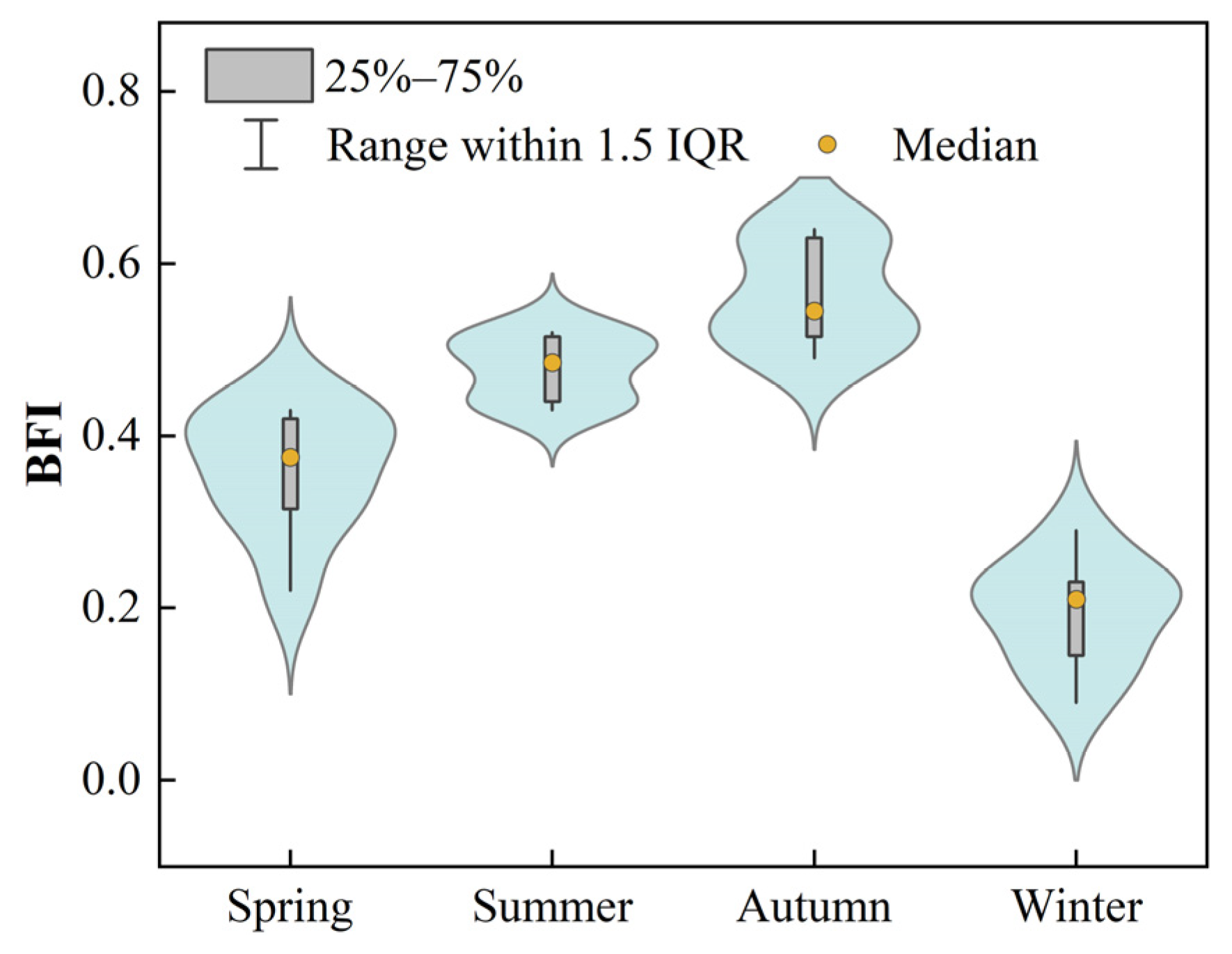
3.2.2. Analysis of Seasonal Scale Evolution Patterns

The seasonal variations in the BFI are illustrated in Figure 9, which presents the probability density estimation of the data. The BFI distribution appears relatively symmetrical, with BFI in spring and summer following a normal distribution, while autumn and winter exhibit a skewed distribution. Based on median trends, the seasonal BFI ranks as follows: autumn > summer > spring > winter. Examining the boxplots size reveals that autumn has the highest dispersion, whereas summer has the lowest. The mean BFI values for spring, summer, autumn, and winter are 0.36, 0.48, 0.56, and 0.19, respectively. The BFI ranged from 0.19 to 0.56, with an average value of 0.40, suggesting that approximately 40% of the long-term runoff in the Upper Emuer River Basin may originate from groundwater discharge and other delayed sources. Summer BFI exhibited fluctuations due to significant variations in streamflow driven by rainfall changes in June, which led to corresponding variations in baseflow. In contrast, autumn and winter displayed more stable trends. The coefficients of variation for the seasonal BFI were 0.19 (spring), 0.07 (summer), 0.10 (autumn), and 0.31 (winter). The minimum and maximum BFI values were 0.09 (winter) and 0.64 (autumn), respectively.

Trend analysis and abrupt change detection of seasonal BFI from 2005 to 2012 were presented in Figure 10, illustrating the temporal characteristics of the data series. The ${\mathbf{Z}}_{\mathbf{M}\mathbf{K}}$ for spring, summer, autumn, and winter were 0.866, −0.371, 0.619, and −0.371, respectively, none of which surpassed the significance threshold of 1.64 (90% significant level). The Mann-Kendall abrupt change detection indicated complexity and irregularity in BFI fluctuations. Specifically, abrupt changes occurred in spring during the years 2007, 2009, and 2011; in summer during 2006 and 2009; in autumn during 2010; and in winter during 2007 and 2010.

3.2.3. Analysis of Monthly Scale Evolution Patterns

The variation in the monthly BFI for the Upper Emuer River Basin is shown in Figure 11. As a high-latitude region, the study area experiences riverbed freezing during winter, which blocks groundwater recharge to baseflow. From April to December, the BFI exhibits a consistent pattern, following a normal distribution. Significant trends in the median lines of the boxplots can be observed, with the median for August being notably higher than that for April. The average BFI in August is elevated, and the interquartile range (IQR) is widest, indicating higher dispersion and greater variability. In contrast, December shows the narrowest IQR, reflecting lower dispersion and higher stability. The multi-year average monthly BFI reaches its maximum value (0.88) in August and its minimum (0.03) in April, with an overall average of 0.43. Due to the delayed response of baseflow originating from shallow aquifers, July exhibits higher baseflow influenced by prior precipitation events, whereas rapid interflow and surface runoff are primarily driven by immediate precipitation events. By September, during the late flood season, the accumulated slow interflow in the basin results in a higher BFI. The coefficient of variation for the BFI ranges from 0.62 in April to 0.10 in June, indicating greater dispersion in April and June.

The trend analysis of monthly BFI values for the Upper Emuer River is summarized in

Table 2. Mann-Kendall test of interannual monthly BFI.

Month	${\mathbf{Z}}_{\mathbf{M}\mathbf{K}}$	Trend	Significance Test
April	0.37115	Increase	Non-Significant
May	1.1135	Increase	Non-Significant
June	1.3609	Increase	Non-Significant
July	0.12372	Increase	Non-Significant
August	−2.3506	Decrease	Significant
September	1.1135	Increase	Non-Significant
October	0.37115	Increase	Non-Significant
November	−0.37115	Decrease	Non-Significant
December	−0.86603	Decrease	Non-Significant

, illustrating the variation characteristics of the BFI time series. From April to July and from September to October, the BFI shows an upward trend, while August, November, and December display a downward trend. Notably, in August, the BFI passes the 95% significance test with a ${\mathbf{Z}}_{\mathbf{M}\mathbf{K}}$ of −2.35, indicating a significant decreasing trend. Similar to the variation characteristics of baseflow, the BFI demonstrates irregular patterns of abrupt changes across different months. Specifically, abrupt changes occurred in April and May in 2007; in June, abrupt changes were observed in 2007 and 2008; in July, changes were noted in 2006, 2008, and 2011. In August, an abrupt change took place in 2008, while September showed changes in 2006, 2008, and 2009. Additionally, abrupt changes were recorded in October and December in 2010, and for November, changes were observed in 2007, 2009, and 2010.

3.3. Analysis of Influencing Factors of Baseflow in the Snowmelt Period

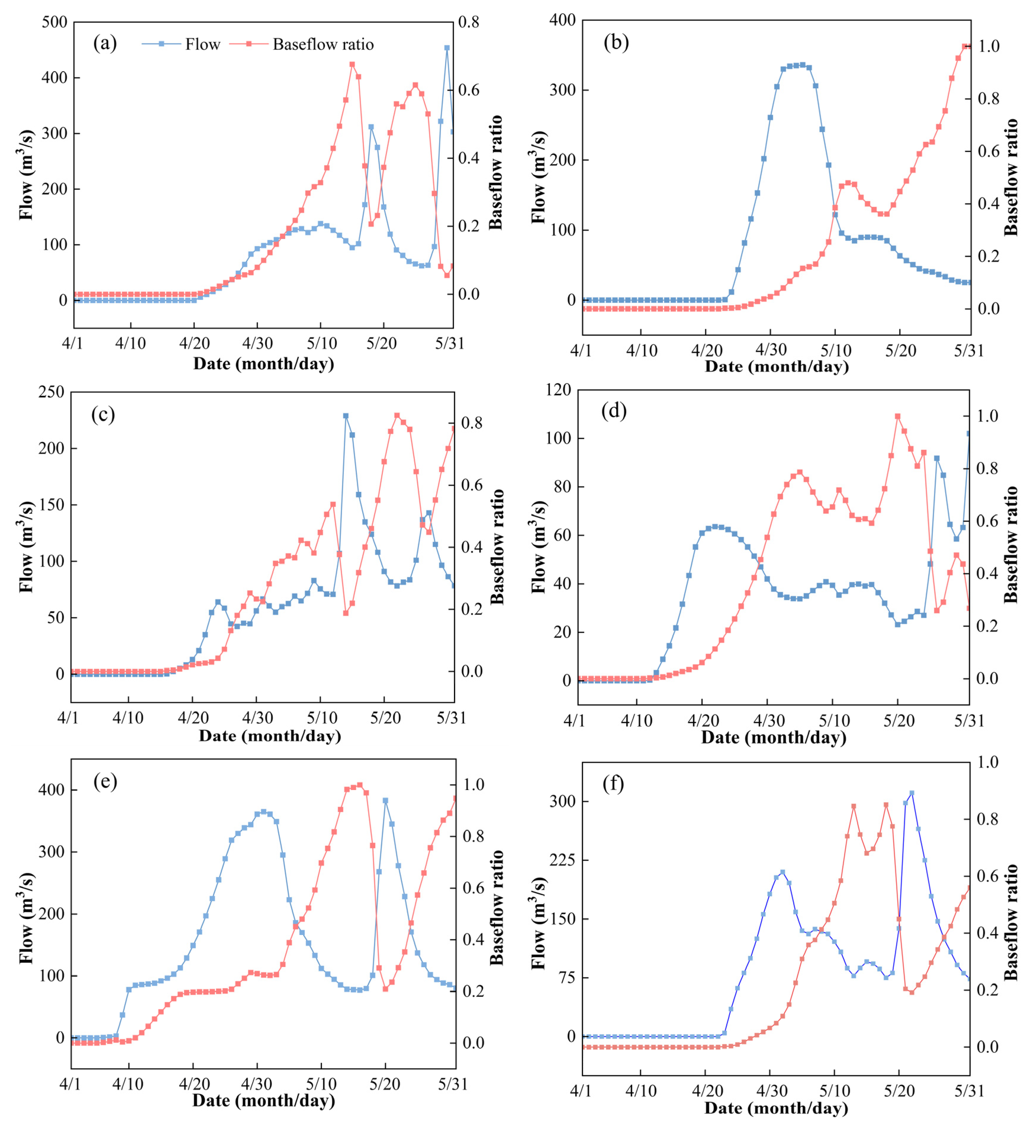
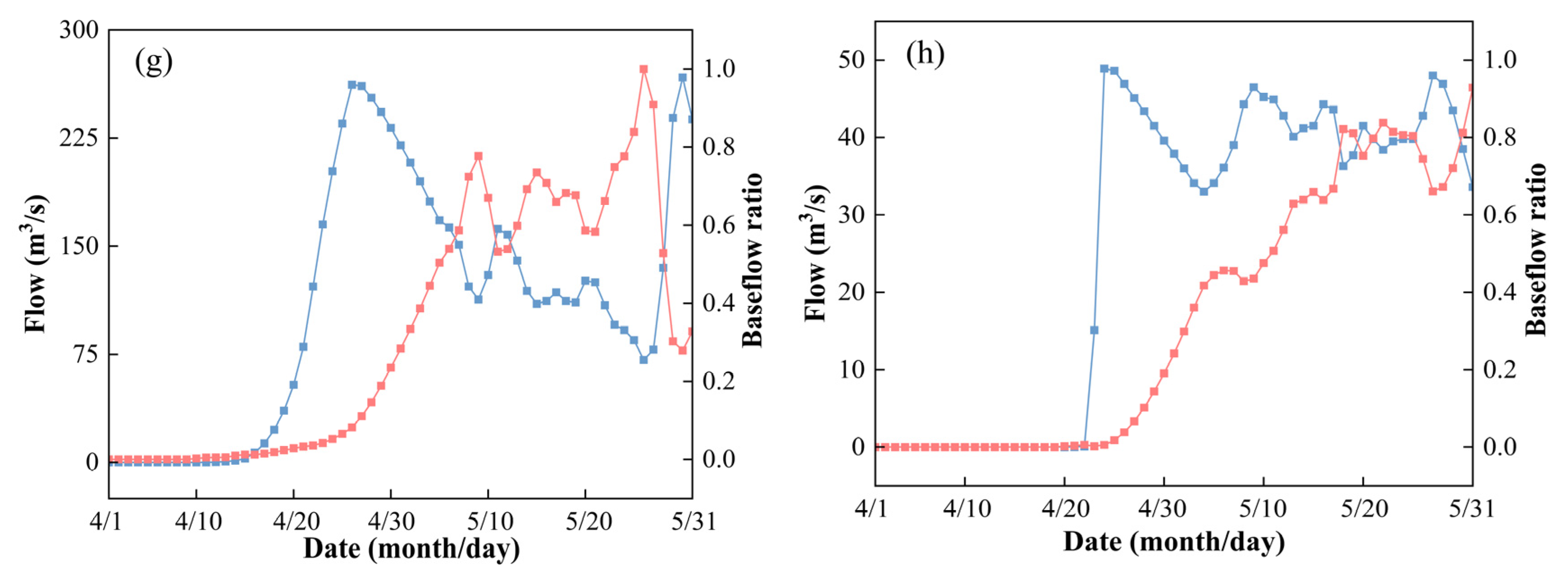
3.3.1. Division of the Snowmelt Period

Using the Eckhardt recursive digital filtering method, we calculated the daily baseflow for the Upper Emuer River Basin from 2005 to 2012. A process curve illustrating the relationship between the BFI and observed flow was generated, where the BFI represents the ratio of baseflow to total runoff. Based on the variation patterns observed in these two process curves, the BFI can serve as an important indicator for distinguishing the beginning time and the end of the snowmelt runoff period. According to temperature changes, snowmelt in the Upper Emuer River typically occurs between April and May. The curves depicting the baseflow ratio and total flow from 1 April to 31 May are shown in Figure 12. The time series curve of the baseflow ratio displays a distinct upward trend, with peak values emerging in mid-to-late April, reaching their maximum around early May, and then declining with oscillatory fluctuations. This curve reflects the contribution of baseflow, predominantly driven by snowmelt, to river discharge. When the baseflow ratio reaches its trough, the proportion of baseflow in total runoff is minimal. This is due to the impermeable frozen soil layer in the watershed, which restricts infiltration during the early snowmelt period. At this stage, the frozen soil near the surface prevents infiltration, leading to more surface runoff or shallow soil moisture while river discharge remains low, marking the onset of snowmelt.

As the temperature rises, the thawing of the frozen soil leads to the contraction of the impermeable layer, and the thickness of the unsaturated zone increases. During this stage, interflow begins to develop, but significant replenishment of deep groundwater is unlikely, resulting in negligible baseflow contributions. As snowmelt progresses, the rapid response of infiltration decreases, resulting in increased interflow, while the contribution of snowmelt to baseflow becomes more pronounced. Meltwater begins to infiltrate through fractures in the frozen soil, replenishing subsurface runoff, which raises the baseflow ratio and forms the first peak. Once the snow has entirely melted, surface runoff and interflow generated by snowmelt gradually disappear, and hillside subsurface flow and groundwater recharge dominate, forming the second peak. This phase marks the end of the snowmelt period. Using the baseflow ratio to delineate the start and end dates of snowmelt, the critical time points were identified based on significant troughs in the runoff process curves for the sample years. The start and end dates of snowmelt from 2005 to 2012 for the Upper Emuer River Basin are summarized in

Table 3. Statistics of snowmelt periods from 2005 to 2012.

Year	Snowmelt Start Date	Snowmelt End Date
2005	21 April	25 May
2006	23 April	30 May
2007	18 April	31 May
2008	12 April	20 May
2009	6 April	31 May
2010	23 April	19 May
2011	10 April	26 May
2012	20 April	20 May

. Snowmelt typically begins around mid-April, with a few instances of earlier onset, such as 6 April in 2009. Approximately 37.5% of snowmelt events began in late April, with the latest onset recorded on 23 April 2006. The multi-year average start date for snowmelt is 17 April. Snowmelt typically ends in late May, with the earliest cessation on 19 May and the latest on 5 May. The multi-year average end date is 25 May. The duration of the snowmelt period ranges from a minimum of 26 days (2010) to a maximum of 56 days (2009), with an average duration of 40 days across the study period.

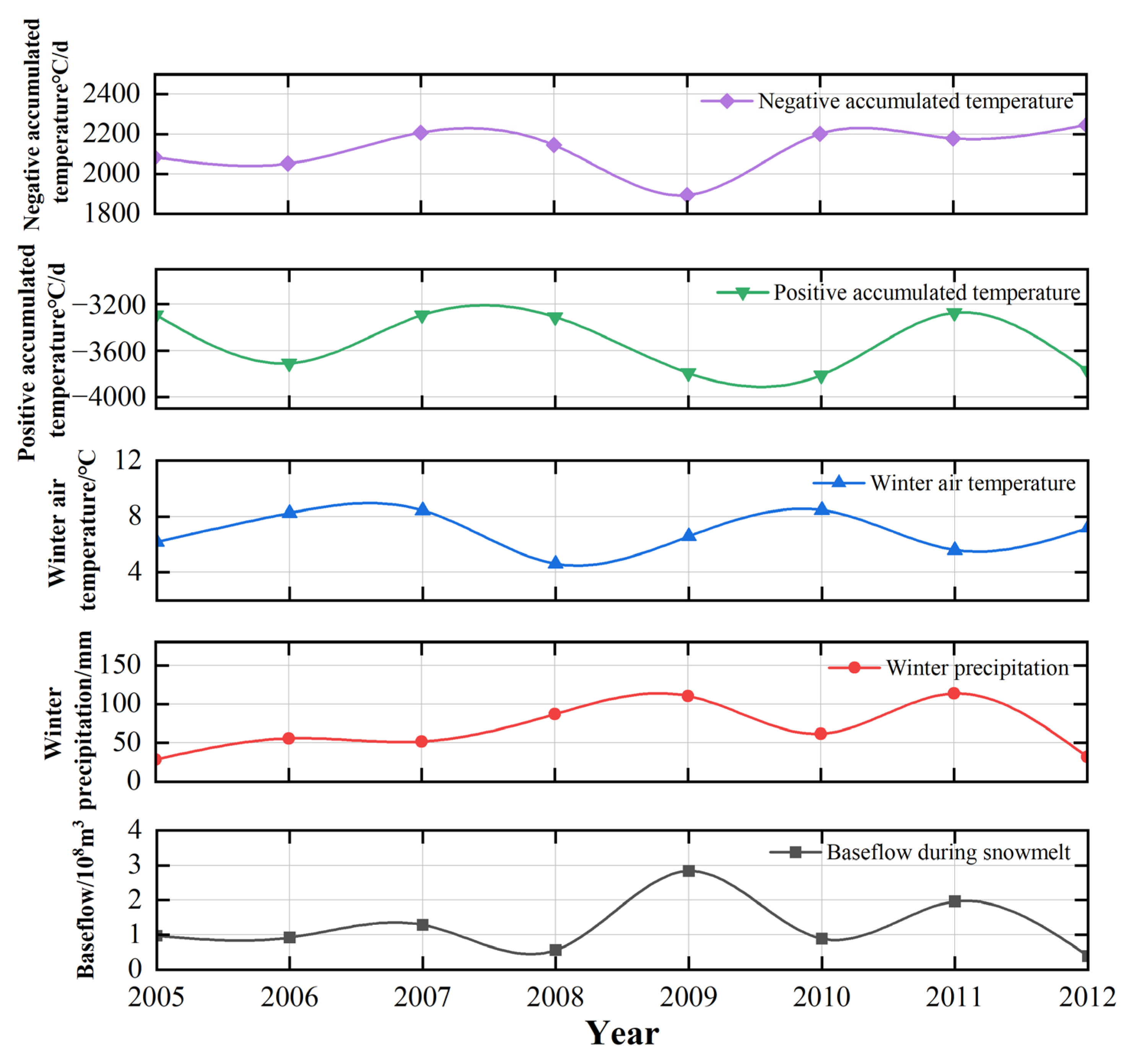
3.3.2. Analysis of Influencing Factors of Baseflow

Climate change plays a crucial role in understanding baseflow dynamics in high-latitude cold regions. As global warming progresses, changes in precipitation and temperature are expected to alter runoff patterns and snow accumulation, which in turn may trigger various effects such as permafrost thawing and glacier retreat [58,59]. Both global climate change and human activities have significant impacts on the hydrological cycle in these cold regions [60]. Figure 13 illustrates the interannual variations in annual positive and negative accumulated temperature, winter air temperature, winter precipitation, and baseflow during the snowmelt season (measured in terms of flow, 10⁸ m³) from 2005 to 2012. The negative accumulated temperature in the Upper Emuer River Basin ranged from −3275.8 °C/d to −3813.2 °C/d, while the positive accumulated temperature ranged from 1894 °C/d to 2245.9 °C/d. Both temperature and precipitation exhibited non-significant increasing trends. The figure also reveals that baseflow during the snowmelt season and winter precipitation shows similar magnitudes of variation.

To further examine the sensitivity of baseflow to climatic factors, key variables such as precipitation and winter air temperature were selected for correlation analysis. The strength of the correlation coefficients quantifies the relationships between these factors. Pearson correlation analysis was employed to calculate the correlation coefficients between meteorological factors and baseflow, with significance testing conducted to assess these relationships, as shown in

Table 4. Correlation between baseflow and climatic factors during the snowmelt period.

Climate Factor	Snowmelt Season Baseflow	Climate Factor	Snowmelt Season Baseflow
Winter air Temperature (°C)	−0.105	Winter Precipitation (mm)	0.724 *
Negative Accumulated Temperature (°C·d)	−0.052	Positive Accumulated Temperature (°C·d)	−0.676

Note: * The correlation was significant at the 0.05 level (double-tailed).

. The correlation strength between baseflow and climatic factors is ranked as follows: winter precipitation > positive accumulated temperature > winter air temperature > negative accumulated temperature. Among these, baseflow showed the strongest positive correlation with winter precipitation (R = 0.724), which was statistically significant at the 0.05 level. Additionally, baseflow was negatively correlated with positive and negative accumulated temperature, as well as winter air temperature. In cold regions, an increase in positive accumulated temperature accelerates snowmelt, enhancing evapotranspiration, which in turn reduces soil moisture and groundwater storage, thereby weakening baseflow recharge. On the other hand, an increase in negative accumulated temperature intensifies freezing processes, inhibiting groundwater recharge and baseflow generation. Cold conditions further slow the exchange between surface water and groundwater, ultimately leading to reduced baseflow.

4. Discussion

The baseflow variation in high-latitude cold regions is mainly influenced by air temperature, precipitation, and snowmelt processes. This study reveals that the baseflow in the Upper Emuer River Basin exhibits clear seasonal variations, with a significant increasing trend in spring and summer, primarily driven by snowmelt and precipitation. Similar findings have been reported by Zhang et al. [61], who analyzed the baseflow characteristics in the source region of the Yellow River using four improved baseflow separation methods. Their study suggested that areas with substantial snow cover significantly enhance spring baseflow. Likewise, Murray et al. [62] found that the summer baseflow (June to September) in Northwestern Canada showed a significant increase from 1989 to 2019, highlighting the cumulative effects of summer rainfall and the gradual release of groundwater. These findings indirectly support the reliability of our results.

Human activities have significantly impacted hydrological processes at both global and regional scales [63]. The Emuer River Basin is located deep within the Greater Khingan Range Mountains, characterized by extensive coverage of pristine forests. As a result, the influence of human activities on hydrological processes in this basin is relatively limited. Zhang et al. [64] concluded that climate change predominantly controlled runoff changes in the Upper Heilongjiang (Amur) River Basin from 1988 to 2017. Nevertheless, future studies should consider the potential indirect impacts of climate change on vegetation and soil characteristics, which may affect long-term groundwater recharge [65].

On the other hand, there are some uncertainties associated with the methods and data used in this study. The baseflow separation method employed may introduce errors during transitional periods such as the onset of snowmelt. The Mann-Kendall method used for detecting trends and abrupt changes is sensitive to the length of the time series data. Although the study considered climatic factors such as precipitation and temperature, factors like soil moisture and permafrost changes may introduce additional uncertainties. Future research should focus on employing multiple methodologies, incorporating more influencing factors, and extending observational data series to reduce these uncertainties and enhance the robustness of baseflow analysis in high-latitude cold regions.

5. Conclusions

This study investigated the evolution of baseflow and the baseflow index (BFI) in the high-latitude cold region of the Upper Emuer River Basin from 2005 to 2012, analyzing their relationships with climatic factors. The main findings are as follows:

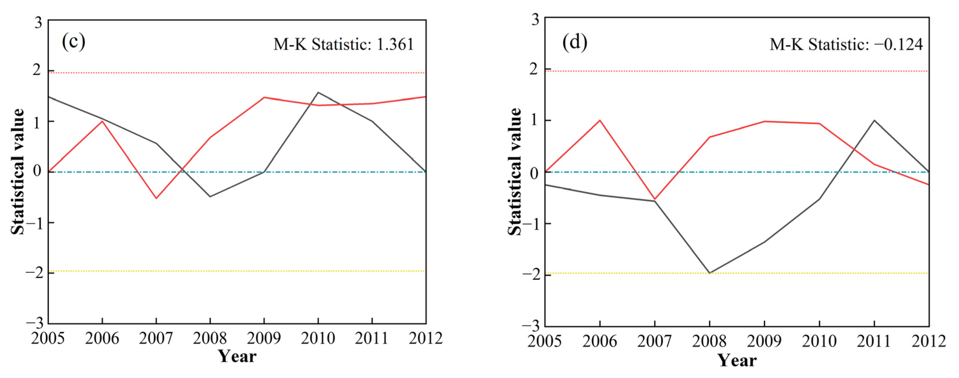
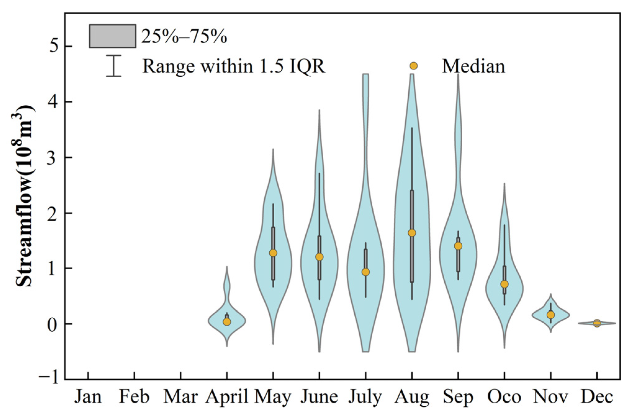
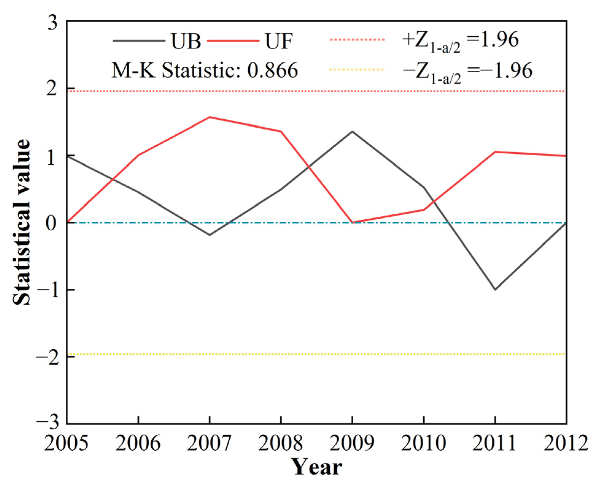
• Runoff variation was more pronounced than baseflow, with greater dispersion, whereas baseflow exhibited a more concentrated distribution. Annual baseflow showed abrupt changes in 2006 and 2008. Seasonally, baseflow increased in autumn, while summer and winter exhibited non-significant declines. Abrupt changes occurred in spring, summer, and autumn in 2008. The most substantial and minimum baseflow variations were observed in August and the winter months (January, February, and March), respectively.
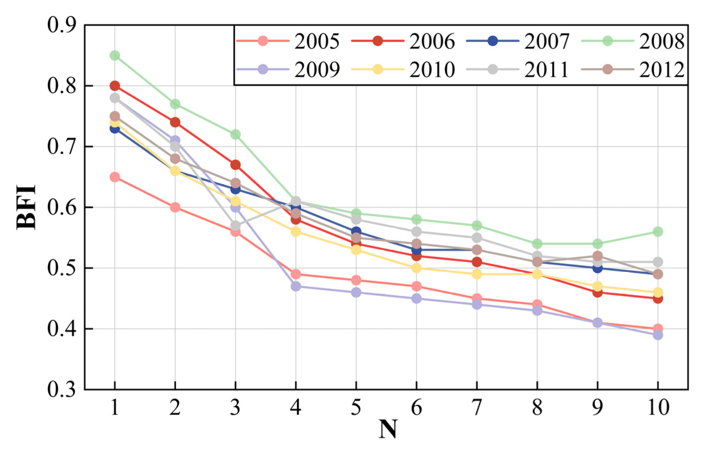
• The BFI ranged from 0.19 to 0.56, with an average value of 0.40, indicating that approximately 40% of the long-term runoff originated from groundwater discharge and other delayed sources. The annual BFI was 0.607. The interannual seasonal BFI exhibits minimal variability and remains relatively stable during the summer and winter months. In contrast, the interannual monthly average BFI peaks in August and shows greater dispersion than in other months.
• The snowmelt period, identified by comparing baseflow ratio and observed runoff curves, lasted an average of 40 days. The Pearson correlation analysis indicated that the snowmelt season baseflow was most strongly influenced by winter precipitation, followed by positive accumulated winter air temperature, and negative accumulated temperature. A strong positive correlation (R = 0.724) was found between baseflow and winter precipitation during the snowmelt season.

The results of this study provide valuable insights into the mechanisms of baseflow generation and its temporal patterns in high-latitude cold regions. In particular, the significant influence of snowmelt on baseflow highlights the importance of monitoring winter precipitation and temperature for accurately predicting spring baseflow. Moreover, the findings contribute to understanding the disaster-causing mechanisms of ice-jam flooding in rivers during the spring season in high-latitude cold regions, providing scientific support for flood prevention and disaster risk management in such environments. Future research can integrate these findings with hydrological models to enhance prediction accuracy and support adaptive water resource management under changing climatic conditions.

References

- Huang, Y.T.; Zhang, L.J.; Li, Y.S.; Ren, C.; Pan, T.; Zhang, W.S.; Zhang, F.; Li, C.Y.; Gu, J.K.; Liu, J. Characteristics of the Northern Hemisphere cold regions changes from 1901 to 2019. Sci. Rep. 2023, 13, 3879. [Google Scholar] [CrossRef] [PubMed]
- Xiang, B.; Liu, E.L.; Yang, L.X. Influences of freezing-thawing actions on mechanical properties of soils and stress and deformation of soil slope in cold regions. Sci. Rep. 2022, 12, 5387. [Google Scholar] [CrossRef] [PubMed]
- Dong, Y.Y.; Zhai, J.Q.; Zhao, Y.; Liu, Z.W.; Yang, Q.; Jiang, S.; Lv, Z.Y.; Yan, D.Y.; Liu, K.; Ding, Z.Y. Impacts of large-scale circulation patterns on the temperature extremes in the cold regions of China with global warming. Front. Earth Sci. 2023, 11, 1120800. [Google Scholar] [CrossRef]
- Javadinejad, S.; Dara, R.; Jafary, F. Climate Change Scenarios and Effects on Snow-Melt Runoff. Civ. Eng. J. Tehran 2020, 6, 1715–1725. [Google Scholar] [CrossRef]
- Zhou, Y.Y.; Xu, Y.J.; Xiao, W.H.; Wang, J.H.; Huang, Y.; Yang, H. Climate Change Impacts on Flow and Suspended Sediment Yield in Headwaters of High-Latitude RegionsA Case Study in China’s Far Northeast. Water 2017, 9, 966. [Google Scholar] [CrossRef]
- Sharma, S.; Mujumdar, P.P. Baseflow significantly contributes to river floods in Peninsular India. Sci. Rep. 2024, 14, 1251. [Google Scholar] [CrossRef]
- Wang, J.Y.; Shrestha, N.K.; Delavar, M.A.; Meshesha, T.W.; Bhanja, S.N. Modelling Watershed and River Basin Processes in Cold Climate Regions: A Review. Water 2021, 13, 518. [Google Scholar] [CrossRef]
- Singh, S.K.; Pahlow, M.; Booker, D.J.; Shankar, U.; Chamorro, A. Towards baseflow index characterisation at national scale in New Zealand. J. Hydrol. 2019, 568, 646–657. [Google Scholar] [CrossRef]
- Qin, J.; Ding, Y.J.; Han, T.D.; Liu, Y.X. Identification of the Factors Influencing the Baseflow in the Permafrost Region of the Northeastern Qinghai-Tibet Plateau. Water 2017, 9, 666. [Google Scholar] [CrossRef]
- Mao, B.Y.; Wang, X.H.; Jia, S.Q.; Liu, Z.J. Multi-methods to investigate the baseflow: Insight from watershed scale spatiotemporal variety perspective. Ecol. Indic. 2024, 158, 111573. [Google Scholar] [CrossRef]
- Chang, Z.H.; Gao, H.K.; Yong, L.L.; Wang, K.; Chen, R.S.; Han, C.T.; Demberel, O.; Dorjsuren, B.; Hou, S.G.; Duan, Z. Projected future changes in the cryosphere and hydrology of a mountainous catchment in the upper Heihe River, China. Hydrol. Earth Syst. Sci. 2024, 28, 3897–3917. [Google Scholar] [CrossRef]
- Singh, V.; Jain, S.K.; Shukla, S. Glacier change and glacier runoff variation in the Himalayan Baspa river basin. J. Hydrol. 2021, 593, 125918. [Google Scholar] [CrossRef]
- Zhao, H.L.; Li, H.Y.; Xuan, Y.Q.; Bao, S.S.; Cidan, Y.; Liu, Y.Y.; Li, C.H.; Yao, M.C. Investigating the critical influencing factors of snowmelt runoff and development of a mid-long term snowmelt runoff forecasting. J. Geogr. Sci. 2023, 33, 1313–1333. [Google Scholar] [CrossRef]
- Cho, E.; McCrary, R.R.; Jacobs, J.M. Future Changes in Snowpack, Snowmelt, and Runoff Potential Extremes Over North America. Geophys. Res. Lett. 2021, 48, e2021GL094985. [Google Scholar] [CrossRef]
- Uzun, S.; Tanir, T.; Coelho, G.D.; de Lima, A.D.; Cassalho, F.; Ferreira, C.M. Changes in snowmelt runoff timing in the contiguous United States. Hydrol. Process. 2021, 35, e14430. [Google Scholar] [CrossRef]
- Feng, M.M.; Zhang, W.G.; Zhang, S.Q.; Sun, Z.Y.; Li, Y.; Huang, Y.Q.; Wang, W.J.; Qi, P.; Zou, Y.C.; Jiang, M. The role of snowmelt discharge to runoff of an alpine watershed: Evidence from water stable isotopes. J. Hydrol. 2022, 604, 127209. [Google Scholar] [CrossRef]
- Kumar, R.; Manzoor, S.; Vishwakarma, D.K.; Al-Ansari, N.; Kushwaha, N.L.; Elbeltagi, A.; Sushanth, K.; Prasad, V.; Kuriqi, A. Assessment of Climate Change Impact on Snowmelt Runoff in Himalayan Region. Sustainability 2022, 14, 1150. [Google Scholar] [CrossRef]
- Gao, Z.; Zhang, C.; Liu, W.; Niu, F.; Wang, Y.; Lin, Z.; Yin, G.; Ding, Z.; Shang, Y.; Luo, J. Extreme degradation of alpine wet meadow decelerates soil heat transfer by preserving soil organic matter on the Qinghai–Tibet Plateau. J. Hydrol. 2025, 653, 132748. [Google Scholar] [CrossRef]
- Tian, L.; Li, H.Y.; Li, F.P.; Li, X.B.; Du, X.Q.; Ye, X.Y. Identification of key influence factors and an empirical formula for spring snowmelt-runoff: A case study in mid-temperate zone of northeast China. Sci. Rep. 2018, 8, 16950. [Google Scholar] [CrossRef]
- Tananaev, N.; Lotsari, E. Defrosting northern catchments: Fluvial effects of permafrost degradation. Earth-Sci. Rev. 2022, 228, 103996. [Google Scholar] [CrossRef]
- Liu, W.; Shang, Y.; Li, G.; Gao, K.; Zhang, H.; Sheng, J. Seasonal Freeze-Thaw Behavior of Ground in Mid-Latitude Cold Regions: A Case Study in Bei’an County, Heilongjiang Province. Front. Earth Sci. 2025, 13, 1566593. [Google Scholar] [CrossRef]
- Shahid, M.; Rahman, K.U.; Haider, S.; Gabriel, H.F.; Khan, A.J.; Pham, Q.B.; Pande, C.B.; Linh, N.T.T.; Anh, D.T. Quantitative assessment of regional land use and climate change impact on runoff across Gilgit watershed. Environ. Earth Sci. 2021, 80, 743. [Google Scholar] [CrossRef]
- Kulik, A.V.; Gordienko, O.A. Conditions of Snowmelt Runoff Formation on Slopes in the South of the Volga Upland. Eurasian Soil Sci. 2022, 55, 36–44. [Google Scholar] [CrossRef]
- Yang, W.C.; Jin, F.M.; Si, Y.J.; Li, Z. Runoff change controlled by combined effects of multiple environmental factors in a headwater catchment with cold and arid climate in northwest China. Sci. Total Environ. 2021, 756, 143995. [Google Scholar] [CrossRef]
- Connon, R.F.; Chasmer, L.; Haughton, E.; Helbig, M.; Hopkinson, C.; Sonnentag, O.; Quinton, W.L. The implications of permafrost thaw and land cover change on snow water equivalent accumulation, melt and runoff in discontinuous permafrost peatlands. Hydrol. Process. 2021, 35, e14363. [Google Scholar] [CrossRef]
- Zheng, G.H.; Yang, Y.T.; Yang, D.W.; Dafflon, B.; Yi, Y.H.; Zhang, S.L.; Chen, D.L.; Gao, B.; Wang, T.H.; Shi, R.J.; et al. Remote sensing spatiotemporal patterns of frozen soil and the environmental controls over the Tibetan Plateau during 2002–2016. Remote Sens. Environ. 2020, 247, 111927. [Google Scholar] [CrossRef]
- Shang, Y.; Cao, Y.; Li, G.; Gao, K.; Zhang, H.; Sheng, J.; Chen, D.; Lin, J. Characteristics of meteorology and freeze-thaw in high-latitude cold regions: A case study in Da Xing’anling, Northeast China (2022–2023). Front. Earth Sci. 2025, 12, 1476234. [Google Scholar] [CrossRef]
- Lei, Y.H.; Li, R.; Letu, H.; Shi, J.C. Seasonal Variations of Recharge-Storage-Runoff Process over the Tibetan Plateau. J. Hydrometeorol. 2023, 24, 1619–1633. [Google Scholar] [CrossRef]
- Gao, Z.; Niu, F.; Lin, Z. Effects of permafrost degradation on thermokarst lake hydrochemistry in the Qinghai-Tibet Plateau, China. Hydrol. Process. 2020, 34, 5659–5673. [Google Scholar] [CrossRef]
- Segura, C.; Noone, D.; Warren, D.; Jones, J.A.; Tenny, J.; Ganio, L.M. Climate, Landforms, and Geology Affect Baseflow Sources in a Mountain Catchment. Water Resour. Res. 2019, 55, 5238–5254. [Google Scholar] [CrossRef]
- Cheng, L.; Zhang, L.; Chiew, F.H.S.; Canadell, J.G.; Zhao, F.F.; Wang, Y.P.; Hu, X.Q.; Lin, K.R. Quantifying the impacts of vegetation changes on catchment storage-discharge dynamics using paired-catchment data. Water Resour. Res. 2017, 53, 5963–5979. [Google Scholar] [CrossRef]
- Gnann, S.J.; McMillan, H.K.; Woods, R.A.; Howden, N.J.K. Including Regional Knowledge Improves Baseflow Signature Predictions in Large Sample Hydrology. Water Resour. Res. 2021, 57, e2020WR028354. [Google Scholar] [CrossRef]
- Yu, Q.Y.; Shi, C.; Bai, Y.G.; Zhang, J.H.; Lu, Z.L.; Xu, Y.Y.; Li, W.Z.; Liu, C.S.; Soomro, S.E.H.; Tian, L.; et al. Interpretable baseflow segmentation and prediction based on numerical experiments and deep learning. J. Environ. Manag. 2024, 360, 121089. [Google Scholar] [CrossRef] [PubMed]
- Ramli, I.; Murthada, S.; Nasution, Z.; Achmad, A. Hydrograph separation method and baseflow separation using Chapman Method—A case study in Peusangan Watershed. IOP Conf. Ser. Earth Environ. Sci. 2019, 314, 012026. [Google Scholar] [CrossRef]
- Zhang, Y.R.; He, Y.; Mu, X.M.; Jia, L.P.; Li, Y.L. Base-flow segmentation and character analysis of the Huangfuchuan Basin in the middle reaches of the Yellow River, China. Front. Environ. Sci. 2022, 10, 831122. [Google Scholar] [CrossRef]
- Bosch, D.D.; Arnold, J.G.; Allen, P.G.; Lim, K.J.; Park, Y.S. Temporal variations in baseflow for the Little River experimental watershed in South Georgia, USA. J. Hydrol.-Reg. Stud. 2017, 10, 110–121. [Google Scholar] [CrossRef]
- Eckhardt, K. A comparison of baseflow indices, which were calculated with seven different baseflow separation methods. J. Hydrol. 2008, 352, 168–173. [Google Scholar] [CrossRef]
- Liu, Z.J.; Wang, X.H.; Xu, Y.J.; Mao, B.Y.; Jia, S.Q.; Wang, C.; Lv, Q.Y.; Ji, X.M. Multi-indicators to investigate the spatiotemporal effect of groundwater-lake interaction on lake development: Case study in the largest fresh water lake (Poyang Lake) of China. J. Hydrol. 2025, 650, 132557. [Google Scholar] [CrossRef]
- Qin, J.; Ding, Y.J.; Han, T.D. Quantitative assessment of winter baseflow variations and their causes in Eurasia over the past 100 years. Cold Reg. Sci. Technol. 2020, 172, 102989. [Google Scholar] [CrossRef]
- Wang, X.; Liu, Z.; Xu, Y.J.; Mao, B.; Jia, S.; Wang, C.; Ji, X.; Lv, Q. Revealing nitrate sources seasonal difference between groundwater and surface water in China’s largest fresh water lake (Poyang Lake): Insights from sources proportion, dynamic evolution and driving forces. Sci. Total Environ. 2025, 958, 178134. [Google Scholar] [CrossRef]
- Wang, X.; Ji, X.; Xu, Y.J.; Mao, B.; Jia, S.; Wang, C.; Liu, Z.; Lv, Q. Multi-machine learning methods to predict spatial variation characteristics of total nitrogen at watershed scale: Evidences from the largest watershed (Yangtze River Watershed), Asian. Sci. Total Environ. 2024, 949, 175144. [Google Scholar] [CrossRef] [PubMed]
- Chen, L. Research on Spring Snowmelt Runoff Simulation in Emuer River Basin Based on SWAT Model. Master’s Thesis, HeiLongJiang University, Harbin, China, 2022. (In Chinese) [Google Scholar] [CrossRef]
- Jia, M.H.; Yu, C.G.; Chen, L.; Dai, C.L. Study on runoff change and influencing factors in Emuer River Basin. Gansu Water Resour. Hydropower 2023, 59, 1–5. (In Chinese) [Google Scholar] [CrossRef]
- Xu, D.L. Analysis on hydrologic calculation of Emuer River bridge. For. Sci. Technol. Inf. 2012, 44, 132–134+138. (In Chinese) [Google Scholar]
- Xiao, C.T.; Ye, M.; Wen, Z.G.; Zhao, S.M.; Yang, X.P.; Zhang, W.L. Study on the paleoflora of Emuerhe Group in Mohe Basin. Earth Sci. Front. 2015, 22, 299–309. (In Chinese) [Google Scholar] [CrossRef]
- Xiao, Y.P.; Wen, Z.G.; Zhao, S.M.; Xiao, C.T. Lithostratigraphic division and correlation of Emuerhe Group in Mohe Basin. China Energy Environ. Prot. 2018, 40, 103–108. (In Chinese) [Google Scholar] [CrossRef]
- Nagy, E.D.; Szilagyi, J.; Torma, P. Calibrating the Lyne-Hollick filter for baseflow separation based on catchment response time. J. Hydrol. 2024, 638, 131483. [Google Scholar] [CrossRef]
- Nathan, R.J.; McMahon, T.A. Evaluation of automated techniques for base flow and recession analyses. Water Resour. Res. 1990, 26, 1465–1473. [Google Scholar] [CrossRef]
- Wels, C.; Cornett, R.J.; Lazerte, B.D. Hydrograph separation: A comparison of geochemical and isotopic tracers. J. Hydrol. 1991, 122, 253–274. [Google Scholar] [CrossRef]
- Xie, J.X.; Liu, X.M.; Wang, K.W.; Yang, T.T.; Liang, K.; Liu, C.M. Evaluation of typical methods for baseflow separation in the contiguous United States. J. Hydrol. 2020, 583, 124628. [Google Scholar] [CrossRef]
- Bathke, A.C. A unified approach to nonparametric trend tests for dependent and independent samples. Metrika 2009, 69, 17–29. [Google Scholar] [CrossRef]
- Ahmadi, A.; Daccache, A.; Snyder, R.L.; Suvocarev, K. Meteorological driving forces of reference evapotranspiration and their trends in California. Sci. Total Environ. 2022, 849, 157823. [Google Scholar] [CrossRef] [PubMed]
- Mehta, D.J.; Yadav, S.M. Long-term trend analysis of climate variables for arid and semi-arid regions of an Indian State Rajasthan. Int. J. Hydrol. Sci. Technol. 2022, 13, 191–214. [Google Scholar] [CrossRef]
- Mann, H.B. Nonparametric tests against trend. J. Econom. Soc. 1945, 13, 245–259. [Google Scholar] [CrossRef]
- Kendall, M.G. Rank Correlation Methods; Griffin: London, UK, 1948. [Google Scholar]
- Saedi, J.; Sharifi, M.R.; Saremi, A.; Babazadeh, H. Assessing the impact of climate change and human activity on streamflow in a semiarid basin using precipitation and baseflow analysis. Sci. Rep. 2022, 12, 9228. [Google Scholar] [CrossRef]
- Edelmann, D.; Móri, T.F.; Székely, G.J. On relationships between the Pearson and the distance correlation coefficients. Stat. Probab. Lett. 2021, 169, 108960. [Google Scholar] [CrossRef]
- Lopez-Moreno, J.I.; Pomeroy, J.W.; Alonso-González, E.; Morán-Tejeda, E.; Revuelto, J. Decoupling of warming mountain snowpacks from hydrological regimes. Environ. Res. Lett. 2020, 15, 114006. [Google Scholar] [CrossRef]
- Gao, Z.Y.; Niu, F.J.; Wang, Y.B.; Luo, J.; Yin, G.A.; Shang, Y.H.; Lin, Z.J. Evaluation of the energy budget of thermokarst lake in permafrost regions of the Qinghai-Tibet Plateau. Adv. Clim. Change Res. 2024, 15, 636–646. [Google Scholar] [CrossRef]
- Gao, H.K.; Li, H.; Duan, Z.; Ren, Z.; Meng, X.Y.; Pan, X.C. Modelling glacier variation and its impact on water resource in the Urumqi Glacier No. 1 in Central Asia. Sci. Total Environ. 2018, 644, 1160–1170. [Google Scholar] [CrossRef]
- Zhang, J.; Lan, Y.; Chen, X.S.; Tan, Y.H.; Wu, T.; Lyu, S.; Zhou, Y.Y.; Zhang, Y.Q.; Cheng, L.; Chen, Y.; et al. Baseflow characteristics and drivers in headwater catchment of the Yellow River, Tibetan Plateau. J. Hydrol. Reg. Stud. 2024, 56, 101991. [Google Scholar] [CrossRef]
- Murray, J.; Ayers, J.; Brookfield, A. The impact of climate change on monthly baseflow trends across Canada. J. Hydrol. 2023, 618, 129254. [Google Scholar] [CrossRef]
- Buytaert, W.; Célleri, R.; De Bièvre, B.; Cisneros, F.; Wyseure, G.; Deckers, J.; Hofstede, R. Human impact on the hydrology of the Andean páramos. Earth-Sci. Rev. 2006, 79, 53–72. [Google Scholar] [CrossRef]
- Zhang, K.W.; Ma, K.; Leng, J.W.; He, D.M. Alteration in Hydrologic Regimes and Dominant Influencing Factors in the Upper Heilong-Amur River Basin across Three Decades. Sustainability 2023, 15, 10391. [Google Scholar] [CrossRef]
- Milly, P.C.D.; Dunne, K.A.; Vecchia, A.V. Global pattern of trends in streamflow and water availability in a changing climate. Nature 2005, 438, 347–350. [Google Scholar] [CrossRef] [PubMed]