Scale Effects in Landslide Susceptibility Assessment: Integrating Slope Unit Division and SHAP-Based Interpretability in a Typical River Basin

Abstract

Landslide susceptibility assessment (LSA) plays a pivotal role in regional disaster prevention, particularly in southeastern Tibet, where frequent landslides pose significant threats to human safety and critical infrastructure. However, current LSA approaches face two key challenges: (1) the absence of standardized guidelines for selecting appropriate slope unit scales, which may result in over-smoothing or excessive noise in spatial patterns; and (2) the limited interpretability of machine learning models, which hampers understanding of factor contributions. This study investigates the scale effects of slope unit delineation on LSA in the Yuqu River Basin. Using the r.slopeunits method, six datasets at varying scales were generated to capture terrain heterogeneity. An XGBoost-based framework was applied for susceptibility modeling, with SHAP (Shapley Additive Explanations) used to enhance model interpretability. Results indicate that slope unit scale substantially affects sample distribution, feature representation, and model performance. At the smallest scale (c = 0.05), excessive data redundancy and imbalanced class ratios reduced accuracy (AUC = 0.824). At the largest scale (c = 0.5), spatial heterogeneity was over-smoothed, also impairing performance (AUC = 0.832). The intermediate scale (c = 0.3) performed best, yielding a balanced representation and a mean AUC of 0.856. SHAP analysis highlighted freezing index, relative height, and rainfall as the most influential factors. Notably, susceptibility increased significantly when the freezing index ranged between 1500 and 3000 °C·d and relative height between 500 and 1500 m. Additionally, interactions—such as between the freezing index and slope gradient or fault density—further intensified landslide risk, underscoring the need to consider nonlinear dependencies. By integrating multi-scale modeling with SHAP-based interpretation, this study enhances both the predictive accuracy and transparency of LSA.

1. Introduction

With the rapid development of large-scale infrastructure projects, such as railways and hydropower stations, in western China, landslide disasters have become increasingly frequent along the southeastern edge of the Tibetan Plateau. Between 2000 and 2020, these landslides caused significant damage to transportation and hydropower infrastructure, displaced thousands of residents, and resulted in severe economic losses. This geologically fragile region faces considerable risks due to the interplay of internal factors, such as active tectonics and steep terrain, and external factors, such as deep river incision and extreme climatic events. Accurate landslide susceptibility assessment (LSA) is therefore critical for managing geological disaster risks and informing evidence-based decision-making in the region [1].

Recent advances in machine learning and geospatial technologies have significantly enhanced landslide susceptibility mapping across diverse environments. For instance, Bammou et al. demonstrated the efficacy of ensemble machine learning models in semi-arid regions, achieving high accuracy (AUC > 0.9) by integrating topographic and climatic factors [2]. However, their framework focused on grid-based units and static factor interactions, overlooking the critical role of scale-sensitive terrain partitioning—a limitation particularly acute in high-mountain regions where slope unit heterogeneity dominates landslide dynamics. Similarly, while studies in tectonically active areas have emphasized seismic and hydrological triggers, they rarely address the compounded effects of freeze–thaw cycles and multi-scale spatial representation [3].

As geospatial data continue to grow exponentially, effectively organizing and representing these data in a scale-appropriate manner has become a critical challenge in landslide risk assessment for complex regions. Landslide susceptibility assessment (LSA) requires spatial units that balance terrain heterogeneity and computational feasibility. While slope units outperform grid-based methods in capturing geomorphological processes, their division scale significantly impacts model performance [4,5]. Existing studies lack standardized guidelines for selecting optimal slope unit scales, with overly small units introducing noise (c = 0.05) and large units over-smoothing critical heterogeneity (c = 0.5) [6]. This scale dependency directly affects sample distribution, feature representation, and ultimately the reliability of susceptibility maps, yet remains underexplored in current literature.

XGBoost, a gradient boosting algorithm, excels in handling nonlinear relationships and high-dimensional data, making it particularly suitable for landslide susceptibility modeling [7,8]. However, its “black-box” nature limits understanding of the roles of contributing factors and undermines its practical application [9]. To address this limitation, SHAP has been integrated to improve model interpretability, providing both global and local insights into the contributions of individual factors. The integration of XGBoost and SHAP is increasingly recognized as a paradigm shift in explainable geospatial modeling. For example, in a global meta-analysis, XGBoost-SHAP frameworks improved model interpretability by 30–50% compared to traditional methods, while maintaining > 90% predictive accuracy. Region-specific applications further highlight their synergy: in the Three Gorges Reservoir Area (China), Huang et al. combined XGBoost with SHAP to identify critical thresholds of reservoir water level fluctuations on landslide reactivation [10]. However, existing studies predominantly adopt grid-based or fixed-scale units, neglecting the scale sensitivity of both model performance and factor contributions.

To address the above issues, this study takes the Yuqu River Basin as an example and combines multi-scale slope unit division with SHAP-based interpretation. By systematically evaluating different division scales, it quantifies their effects on prediction accuracy and zoning rationality, ultimately identifying critical thresholds for key factors. The objectives of this study are threefold: (1) To systematically evaluate for the first time the impact of slope unit partitioning scale on landslide susceptibility assessment, providing a solution to the limitation of the lack of standardized partitioning strategies in current research, and optimizing the method for selecting landslide evaluation units; (2) To introduce the SHAP method for both global and local interpretability analysis of the landslide susceptibility evaluation model, revealing the complex mechanisms of landslide conditioning factors from the perspectives of factor contribution and synergistic effects, effectively enhancing the interpretability of machine learning models and filling the gap in research on the ‘black-box’ issue; (3) to propose a dynamic framework that combines multi-scale analysis of LSA with explainable models in high mountain areas. These findings contribute to a deeper understanding of landslide mechanisms in complex terrains and provide a robust framework for improving LSA methods in high mountain regions.

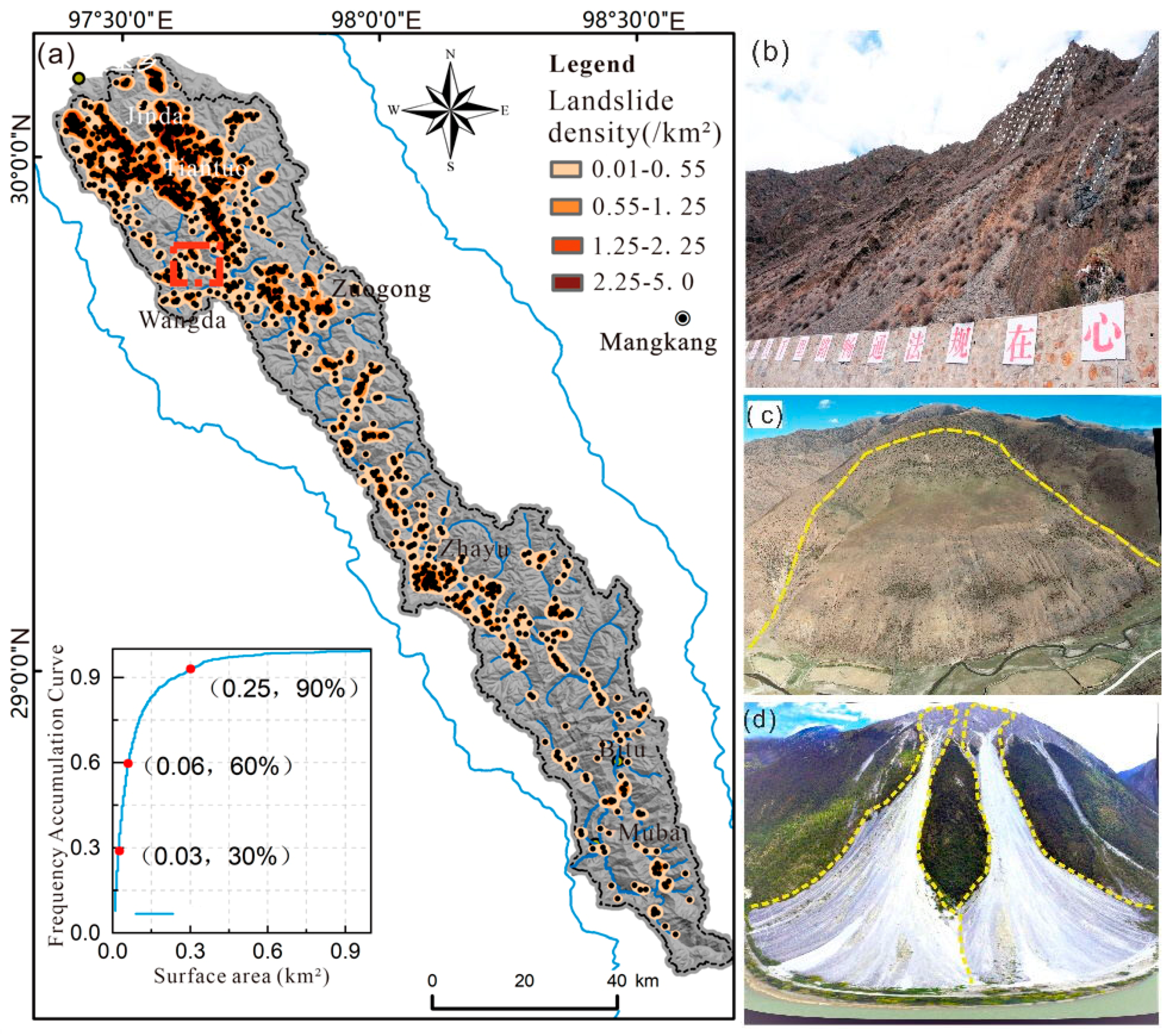
2. Overview of the Study Area

The Yuqu River is a major first-order tributary located on the left bank of the middle Nujiang River, in the southeastern Tibetan Plateau’s Hengduan Mountains. It is geographically situated between 97°30′ E to 98°30′ E longitude and 28° N to 30°30′ N latitude, exhibiting a narrow, elongated shape from northwest to southeast. The total drainage area is approximately 5136 square kilometers, with a river length of 335 km (Figure 1). This basin is located within the steep transition zone where the Qinghai-Tibet Plateau meets the Yunnan-Guizhou Plateau; the Yuqu River Basin exemplifies a high mountain gorge region characterized by complex geological and geomorphological features. Its striking geomorphological heterogeneity is highlighted by elevation variations, ranging from over 5000 m in the northern plateau mountainous areas to approximately 2000 m in the southern gorge regions. The basin encompasses four distinct geomorphological regions: plateau mountainous terrain, expansive plateau valleys, transitional gorge zones, and deeply incised mountain gorges. These regions are shaped by active river incision, high erosion rates, and structural controls, making the basin highly prone to frequent and varied landslide types, including rockslides, debris flows, and rotational failures [11]. The critical role of geomorphological and tectonic conditions in influencing landslide susceptibility has been extensively documented in comparable mountainous regions. For instance, Gong et al. highlighted deep valley incision and steep slopes as contributing triggers in tectonically active terrains, such as the southeastern Tibetan Plateau [12]. In high-mountain collision zones (e.g., the Himalayas), large-scale slope instability is mainly driven by seismic activity and the accumulation of tectonic stress, rather than being solely influenced by topographic factors [13]. Research indicates that the cumulative energy released by repeated high-magnitude earthquakes along the Main Frontal Thrust of the Himalayas gradually weakens the integrity of the rock mass, promoting the formation of extensive fracture networks [14]. These structural weaknesses significantly increase the likelihood of catastrophic slope instability, even in the absence of extreme precipitation or river incision, highlighting the crucial role of seismic-tectonic processes in landslide initiation in this region. These combined processes amplify slope instability, particularly in areas with fractured or weathered rock masses. In the Yuqu River Basin, historical seismic records (e.g., the 2014 Ludian earthquake) further validate that seismic shaking acts as a primary trigger for large-scale landslides, often preceding subsequent failures induced by rainfall or fluvial erosion [15].

Geologically, the Yuqu River Basin lies within the collision zone of the Indian and Eurasian tectonic plates, forming part of the Bangong-Nujiang suture zone. Its lithology comprises Hercynian, Indosinian, and Yanshanian igneous rocks, along with metamorphic and sedimentary units [16]. This diverse lithology results in heterogeneous rock mass conditions, which are especially susceptible to structural influences, such as faulting and folding. The Jiali fault zone (F3), a prominent tectonic feature in the region, is associated with frequent seismic activity, resulting in zones of reduced rock integrity. Studies, including Guzzetti et al., have highlighted the significant impact of geological complexity on regional landslide susceptibility [17].

Fault systems not only weaken rock masses but also interact with hydrological systems, exacerbating slope instability. This interplay of geological and structural factors underscores the high susceptibility of the Yuqu River Basin to frequent landslides. Climatically, the basin experiences significant annual precipitation variability, with most rainfall occurring during the summer monsoon season (July–August). The mean annual precipitation ranges from 200 to 650 mm, with intense rainfall events frequently triggering landslides, especially debris flows and shallow landslides [18]. Freeze–thaw cycles also contribute to slope destabilization during the winter and spring, particularly in higher-elevation areas. Hydrological factors also contribute significantly to landslide activity. The deep fluvial incision of the Yuqu River and its tributaries causes undercutting at slope bases, increasing instability. Similar hydrological influences have been observed in tectonically active river basins, where steep river gradients and active channel erosion intensify landslide risks [19].

The Yuqu River Basin is also characterized by significant tectonic activity due to its location within the Himalayan orogenic belt. Historical seismic records reveal frequent earthquakes with magnitudes ≥ 4.7, with peak ground acceleration (PGA) values ranging from 0.12 g to 0.15 g [15]. Seismic shaking serves as a primary trigger for large-scale landslides in the region, often impacting slopes that are already weakened by geomorphological and climatic factors. For example, landslides triggered by the 2014 Ludian earthquake in a similar geological setting demonstrated the compounded effects of seismic activity on slope failures [20]. In recent years, human activities, such as road construction, hydropower development, and land-use changes, have further exacerbated slope instability. The construction of National Highway 318 and several hydropower stations has significantly altered natural drainage systems, disrupting slope stability throughout the basin. Human-induced modifications, coupled with geological and climatic factors, have increased both the frequency and severity of landslides [17]. This combination of geological, geomorphological, climatic, and anthropogenic factors makes the Yuqu River Basin a critical region for landslide susceptibility studies. Its diverse environmental conditions provide a natural laboratory for testing advanced modeling techniques, particularly those that integrate slope unit-scale analyses with machine learning and interpretability methods.

3. Research Data

The datasets used in this study were sourced from multiple channels, including remote sensing, geological surveys, and field observations. These datasets comprise historical landslide inventories, topographical data, geological and hydrological factors, and anthropogenic variables. To ensure consistency and precision, all data were preprocessed to a unified spatial resolution of 30 m and reprojected into the WGS_1984_UTM_Zone_47N coordinate system.

3.1. Historical Landslide Inventory

A detailed historical landslide inventory for the Yuqu River Basin was established using high-resolution Google Earth imagery interpretation, validated by field observations (Figure 2). A total of 1329 landslide events were identified, including slides, topples, and debris flows. The inventory primarily focused on damage zones and deposition areas, without further differentiation of landslide crowns or back scarp due to the lack of precise morphological data.

The spatial distribution of landslides shows significant heterogeneity, with high concentrations in Tiatuo Town, Wangda Town, and the Zhayu section of the Yuqu River’s main channel, reaching a maximum density of 2.52 events/km². Most of these landslides are small to medium-sized events, with areas ranging from 0.001 to 0.25 km², collectively covering 74.65 a total area of km². These findings align with previous studies, which emphasize the predominance of small-scale landslides in tectonically active zones [1,12]. The most notable recent landslide occurred in August 2014 in Bitu Township, where a massive rockfall blocked the river channel, posing significant risks to hydropower infrastructure and transportation.

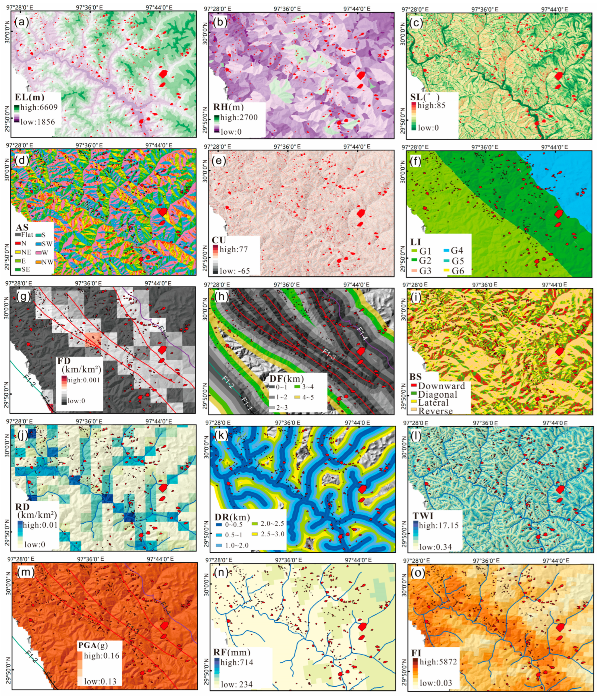
3.2. Influencing Factors

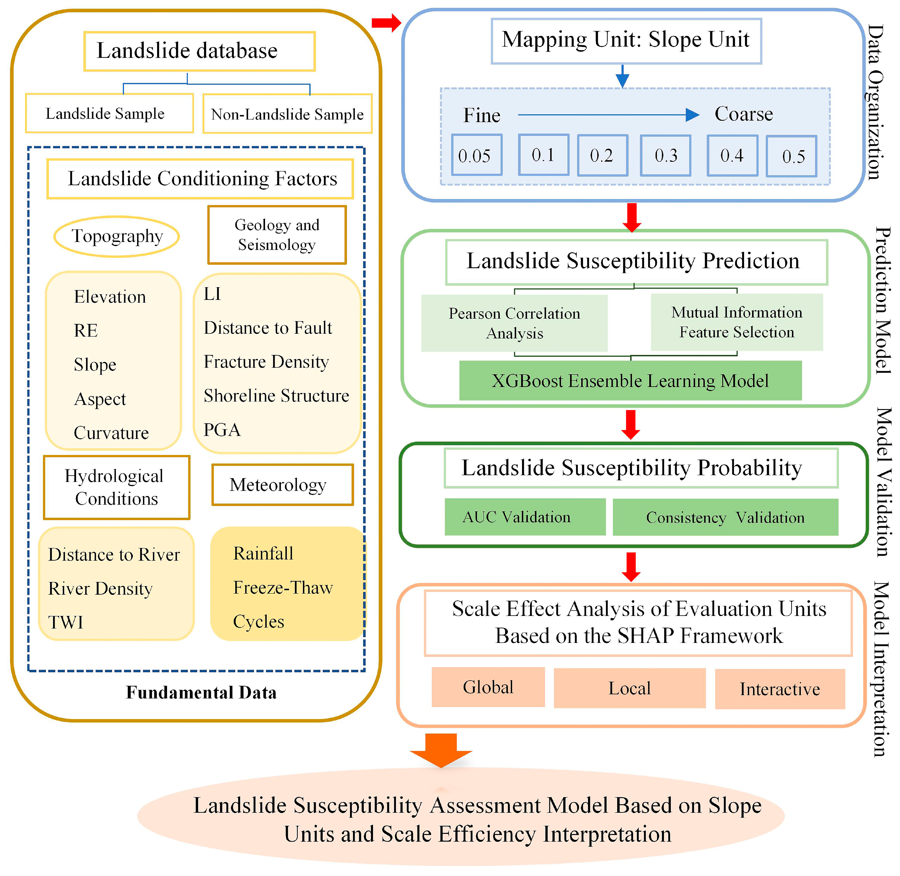
Landslide formation is influenced by a combination of internal and external factors, including topography, lithology, hydrology, and human activities. Considering the regional characteristics of the Yuqu River Basin, 15 contributing factors were identified and categorized into four groups (

Table 1. Categorization, symbolization, data sources, types, and spatial resolution of 15 landslide contributing factors in the Yuqu River Basin.

Causative Factor	Symbol	Data Source	Data Type	Resolution/Scale
Elevation	EL	DEM (2016)	Continuous	30 m
Slope	SL	DEM (2016)	Continuous	30 m
Aspect	AS	DEM (2016)	Discrete	30 m
Curvature	CU	DEM (2016)	Continuous	30 m
Relative Height	RH	DEM (2016)	Continuous	30 m
Lithology	LI	Geological Map (1995–2002)	Discrete	1:200,000
Fault Density	FD	Geological Map (1995–2002)	Continuous	1:200,000
Distance to Faults	DF	Geological Map (1995–2002)	Discrete	1:200,000
PGA	PGA	China Earthquake Administration	Continuous	1:4000
Bank slope	BS	Geological Map (1995–2002)	Discrete	1:200,000
Terrain Wetness Index	TWI	DEM (2016)	Continuous	30 m
Distance to Rivers	DR	National Qinghai-Tibet Plateau Science Data	Discrete	30 m
River Density	RD		Continuous	30 m
Rainfall	RF		Continuous	30 m
Freezing Index	FI		Continuous	30 m

): (1) Topographical factors, including slope angle, aspect, terrain wetness index (TWI), curvature, and relative height. These factors are critical for assessing slope energy and stability. For instance, steeper slopes and greater relative heights are typically associated with higher landslide susceptibility [21]; (2) Geological factors, include lithological formations, fault density, and distance to faults. Lithological variations directly affect slope strength and resistance to failure, while proximity to faults indicates structural weaknesses [22]; (3) Hydrological and climatic factors, including annual rainfall, freezing index, and distance to rivers, were analyzed. Rainfall is a well-established trigger for landslides in monsoonal regions, while freeze–thaw cycles contribute to weakening slopes at higher altitudes [18]; (4) Anthropogenic factors, such as land-use types, distance to roads, and seismic peak ground acceleration (PGA), were incorporated to capture the effects of human activities and seismic disturbances on slope stability [23].

To ensure comparability among variables, all continuous data were standardized using min-max normalization, scaling values to a range between 0 and 1. Pearson correlation coefficients were calculated to detect multicollinearity among factors, and variables with an absolute correlation threshold exceeding 0.7 were excluded. Additionally, a mutual information analysis was conducted to prioritize the factors with the greatest impact on landslide susceptibility, ensuring that only the most representative variables were included in the final model (Figure 3) [24]. The integration of multi-source datasets enables a comprehensive analysis of landslide susceptibility. By combining high-resolution remote sensing data with in situ geological and hydrological information, this study captures both spatial heterogeneity and temporal dynamics. Recent studies emphasize the importance of such integrated datasets in improving the accuracy and reliability of landslide susceptibility models [1,25].

4. Research Methods

This study employed a systematic five-step methodology to evaluate the scale-dependent effects of slope unit division on landslide susceptibility and to analyze the nonlinear contributions and synergistic interactions of contributing factors. The workflow comprised database construction, multi-scale slope unit division, data preprocessing, susceptibility modeling, and model interpretability analysis, as shown in Figure 4.

4.1. Data Preprocessing of Influencing Factors

Fifteen landslide influencing factors, derived from various sources, were standardized into raster format with a spatial resolution of 30 m using the WGS_1984_UTM_Zone_47N projection system. The preprocessing steps were as follows: (1) Continuous numerical factors were normalized to a 0–1 range using the min-max scaling method, while discrete factors retained their original categorical values. (2) The Pearson correlation coefficient method was applied to assess inter-factor correlations. Factors with an absolute correlation coefficient greater than 0.7 were excluded to mitigate multicollinearity. (3) Weakly related or redundant factors were excluded, retaining only those with strong associations to landslide occurrence. Mutual information analysis was utilized to quantify the relationships between contributing factors and landslides by constructing joint probability functions. This comprehensive preprocessing ensured a robust set of influencing factors, incorporating topographical, geological, climatic, and anthropogenic variables to support landslide susceptibility modeling.

4.2. Slope Unit Division

Slope units were delineated using the r.slope.units program developed by Alvioli et al. which is known for its exceptional adaptability to mountainous terrains [26]. The following parameters were configured to generate slope units of varying sizes: Flow accumulation threshold, denoted as ‘t’, with units of 100 × 10⁴ m³, represents concentrated flow areas; Minimum area threshold, denoted as ‘α’, with a unit of 30 × 10⁴ m², represents small sub-basin features; Minimum circular variance of aspect, denoted as ‘c’. Flow accumulation represents the total number of upstream grid cells contributing flow to a given cell in the downslope direction. Grid cells with high flow accumulation values indicate concentrated flow zones and are commonly used to delineate drainage lines and valleys. When the flow accumulation value in a cell exceeds a specified threshold (t), the cell is classified as part of a river channel. This process generates drainage divides that separate the sub-basin into two semi-sub-basins. Each semi-sub-basin is evaluated based on two parameters: minimum area threshold (α) and minimum circular variance of aspect (c). If either of the two criteria is met, the semi-sub-basin is designated as a candidate slope unit. The parameter α defines the minimum allowable area for a slope unit. Semi-sub-basins with areas below α are retained as slope units and are excluded from further iterations. Aspect circular variance measures the directional dispersion of slope aspects within each candidate unit. Lower variance values correspond to more uniform terrain morphology. The c value is a key control on slope unit granularity: smaller values of c produce slope units with higher internal homogeneity, while larger values result in more heterogeneous units. Considering the complex alpine gorge terrain of the Yuqu River Basin, the minimum circular variance of aspect (c) was sequentially set to 0.05, 0.1, 0.2, 0.3, 0.4, and 0.5 to generate six sets of slope units at different levels of spatial resolution. As c increased, the average slope unit area expanded from 0.25 km² to 1.82 km². Among these, the setting of c = 0.3 produced the optimal terrain subdivision, as it achieved the best balance between internal homogeneity and external heterogeneity during the automatic slope unit delineation process [6].

4.3. XGBoost Ensemble Learning Model

The Extreme Gradient Boosting (XGBoost) model, a scalable tree boosting system optimized for speed and performance, was utilized for landslide susceptibility assessment [7]. Its capability to handle nonlinear relationships and high-dimensional data has been widely validated in geohazard prediction, particularly for imbalanced landslide datasets [8,23]. Key features of the model include gradient boosting, which involves iteratively minimizing residuals of weak predictors to improve overall performance, and regularization techniques (L1/L2 norms) to mitigate overfitting by penalizing complex tree structures; the basic principle is illustrated in Figure 5. The model was implemented using Python (Version 3.10)’s Scikit-learn library (Version 1.2. x), with hyperparameter optimization performed through grid search following best practices for geospatial machine learning. For parameter configuration: The learning rate (η) was set between 0.01 and 0.3 to control the step size of updates, balancing convergence speed and overfitting risks [27]. Maximum tree depth was configured between 3 and 10 to manage tree complexity, a range recommended for landslide susceptibility studies to avoid over-specialization [10]. Subsample ratio (0.5–1.0) controlled the proportion of data used in tree construction, enhancing robustness through stochastic gradient boosting [28].

Regularization parameters (λ for L2, α for L1) were tuned to prevent overfitting, with values selected via 5-fold cross-validation [29]. The dataset was split into training (70%) and testing (30%) subsets, adopting stratified sampling to ensure balanced representation of landslide and non-landslide samples [30].

4.4. Landslide Susceptibility Assessment and Validation

Landslide susceptibility was assessed using the Area Under the Curve (AUC) metric of the Receiver Operating Characteristic (ROC) curve, which evaluates classification performance. AUC values approaching 1.0 indicate higher predictive accuracy. Furthermore, the rationality of zoning was assessed by calculating the proportion of historical landslides captured within high-susceptibility zones relative to the total area of these zones. Independent model training and validation were performed 20 times for each of the six slope unit scales to minimize random sampling bias. Landslide susceptibility indices were classified into five categories: Very High (0.8–1.0), High (0.6–0.8), Moderate (0.4–0.6), Low (0.2–0.4), and Very Low (0.0–0.2). The results highlighted the significant influence of slope unit scale on both prediction accuracy and zoning rationality, offering valuable insights for optimizing landslide susceptibility assessment.

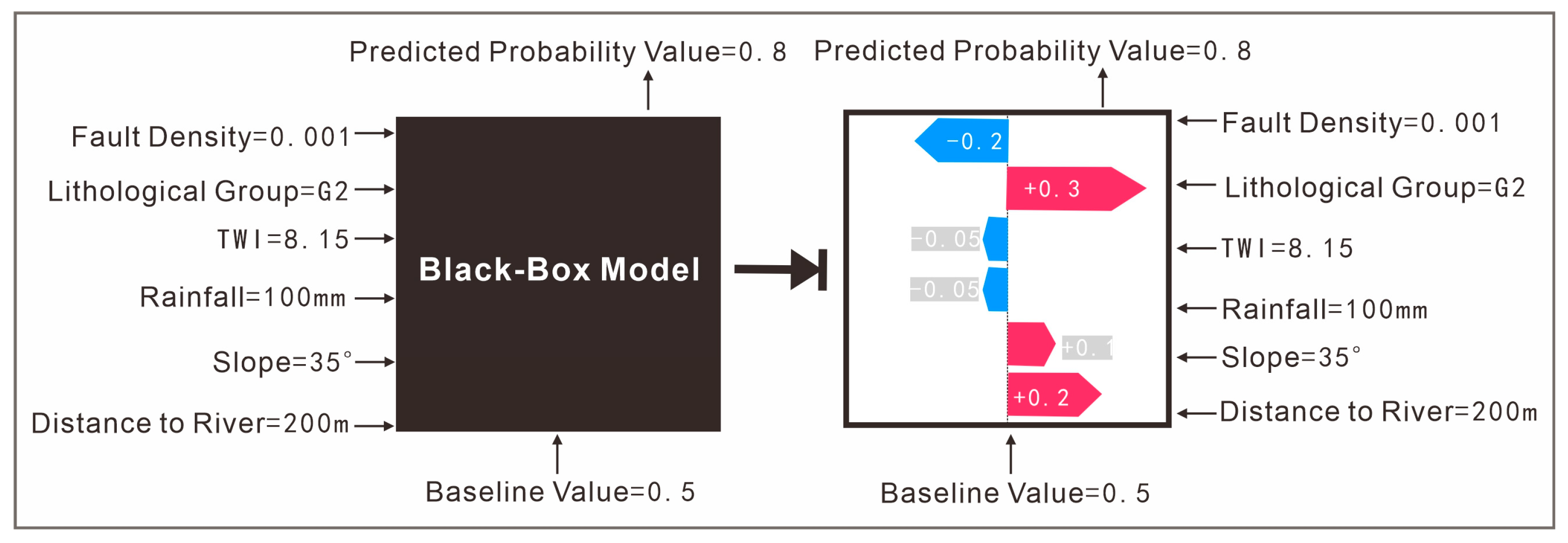
4.5. SHAP Model Interpretability

To investigate the predictive mechanisms of the XGBoost model and clarify the influence of each contributing factor, the SHAP method was employed. Based on game theory, SHAP calculates the marginal contribution of each feature to the model’s predictions.

Its primary benefits include: (1) A global analysis is required to rank the feature importance across the entire dataset. For example, the freezing index, relative height, and rainfall were identified as the dominant contributors to landslide susceptibility. Interactions between factors, such as the freezing index with slope gradient and fault density, revealed critical nonlinear responses. (2) A local analysis is needed to generate force plots and decision plots for specific spatial units, quantifying the positive or negative contributions of individual factors. For instance, the freezing index and relative height frequently showed strong positive contributions in high-susceptibility zones, while rainfall occasionally displayed stabilizing effects in low-susceptibility zones. During model training and testing, each sample generates a prediction value. The contribution of each feature to this prediction is quantified as its SHAP value, calculated using Equation (1):

$${\varphi }_i={\displaystyle \sum _{S\subseteq N\left\{i\right\}}\frac{\left|S\right|!(n-\left|S\right|-1)!}{n!}\left[f(S\cup \left\{i\right\})-f(S)\right]}$$

(1)

Here: ${\varphi }_i$ is the contribution of the $i$ causative factor to the landslide susceptibility prediction. $N$ is the set of all contributing factors. S is a subset of n excluding the ith factor. $f(S\cup \left\{i\right\})$ and $f(S)$ are model predictions with and without the inclusion of the ith influencing factor.

SHAP constructs additive feature attribution models, where the output prediction is defined as the linear sum of input variable contributions, as shown in Equation (2):

$$g(z^{\prime })={\varphi }_0+{\displaystyle \sum _{i=1}^M{\varphi }_i}{z^{\prime }}_i$$

(2)

Here: $g(z^{\prime })$ is the predicted value for a specific sample. M is the number of contributing factors; ${\varphi }_0$ is the mean prediction value for all samples; ${\varphi }_i$ is the SHAP value for the ith factor. A positive ${\varphi }_i$ indicates a positive contribution to landslide susceptibility, while a negative ${\varphi }_i$ denotes a negative contribution. This study employed Python’s SHAP library to compute the SHAP values, systematically analyzing factor contributions and their interactions. The weighted SHAP values clarified the spatial heterogeneity of the contributing factors and their combined effects, overcoming the limitations of traditional statistical methods and providing both theoretical and technical support for landslide susceptibility modeling (Figure 6).

4.6. Research Objectives

Addressing the existing gaps in slope unit scale dependency, model interpretability, and factor categorization, this study proposes an innovative framework for landslide susceptibility assessment (LSA) tailored to high-mountain regions. The research aims to bridge these limitations through three key objectives:

First, to systematically evaluate the influence of slope unit scales (c = 0.05–0.5) on model performance and zoning effectiveness, ensuring an optimal balance between spatial resolution and predictive accuracy. Second, to advance model interpretability by integrating SHAP with multi-scale analysis, allowing for a more transparent and data-driven understanding of nonlinear factor contributions and their interactions. Third, to develop a dynamic factor classification framework that differentiates preparatory and triggering factors in accordance with Nath et al., thereby refining the identification of landslide-driving mechanisms [31].

Compared with traditional grid units, slope units allow for the selection of different partitioning scales based on the specific characteristics of the study area, thereby enabling consideration of the correlations among conditioning factors and between these factors and landslides. Additionally, the SHAP method provides interpretability by quantifying the contribution of each conditioning factor to landslide initiation. This study not only enhances LSA precision but also contributes to a more robust, interpretable outcome.

5. Results

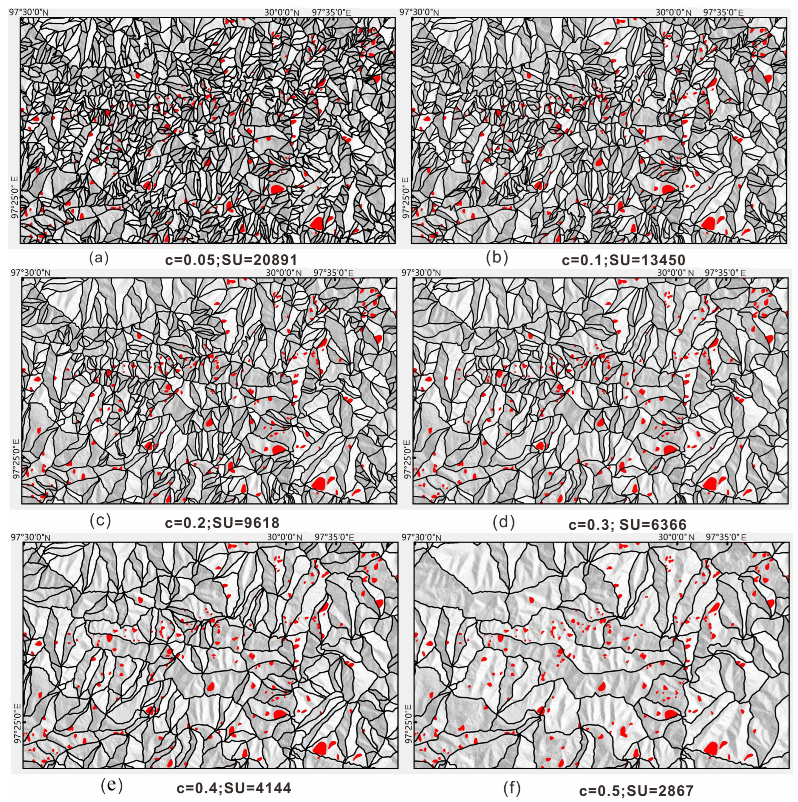
5.1. Results of Slope Unit Division

The characteristics of slope unit divisions at different scales are summarized in

Table 2. Characteristics of slope unit datasets across six division scales (c = 0.05–0.5): Total samples, landslide/non-landslide ratios, and spatial coverage.

Sampling Method	Dataset	Slope Unit Size Parameter (c)
		0.05	0.1	0.2	0.3	0.4	0.5
Centroid-Based	Total Samples	20,891	13,450	9618	6366	4144	2867
	Landslide Units	1077	906	832	756	625	519
	Non-Landslide Units	19,814	12,544	8786	5610	3519	2348

and Figure 7. As the size of the slope units increased, the total number of units decreased significantly. For example, when the circular variance parameter c was set to 0.05, 0.2, and 0.5, the total number of slope units reduced from 20,891 to 9618, and finally, to 2867. Concurrently, the ratio of landslide to non-landslide units improved with larger unit sizes.

Specifically, at c = 0.05, the ratio of landslide to non-landslide units was approximately 1:20, whereas at c = 0.3, this ratio improved to 1:10. These findings suggest that larger slope units help balance the distribution of positive and negative samples, which is essential for training robust machine learning models [10,26].

To scientifically determine the optimal slope unit delineation scale, this study employed a combined supervised and unsupervised evaluation strategy for quantitative validation (Figure 8). First, the Object-level Consistency Error (OCE) was used to evaluate the matching between 30 parameter combinations and 952 reference slope units, with OCE < 0.35 as the standard to screen 15 qualified parameter combinations, effectively eliminating unreasonable unit groups caused by over-segmentation and under-segmentation. Subsequently, the Global Synthesis heterogeneity index (GS) was calculated for qualified combinations, which comprehensively considers the global Moran’s index and global variance, enabling quantification of the balance between the internal homogeneity and the external heterogeneity of slope units. Results indicated that the parameter combination (t = 100 × 10⁴ m³, c = 0.3) achieved the highest GS value of 1.88, significantly superior to the parameter combination (100, 0.1) determined by traditional methods, with a GS value of 1.83, while the latter had an OCE error as high as 0.38, indicating obvious terrain over-segmentation problems. These quantitative evaluation results provide sufficient scientific basis for c = 0.3 as the optimal slope unit delineation scale, ensuring the rationality and reliability of spatial unit selection for subsequent landslide susceptibility assessment.

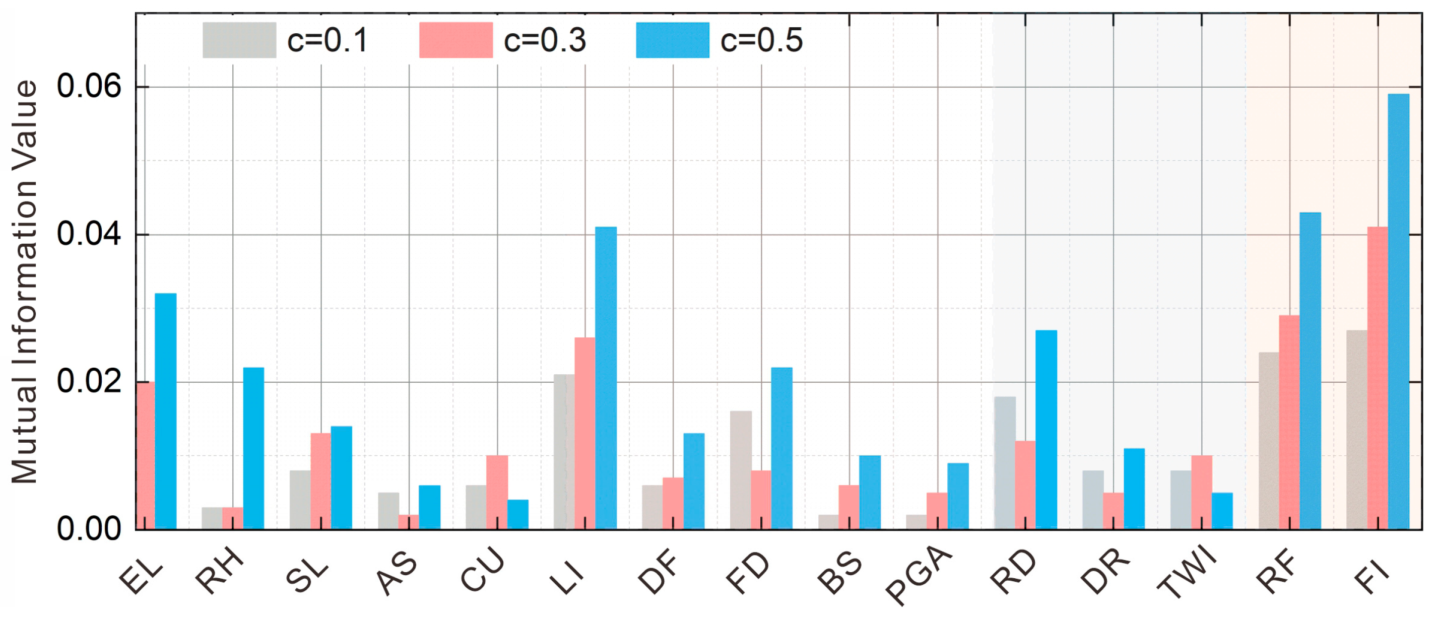
5.2. Influencing Factors Selection

The Pearson correlation coefficient analysis showed that the correlation coefficients among the influencing factors across different slope unit sizes and sampling methods ranged from 0 to 0.6, suggesting no evidence of multicollinearity. Further analysis employed the mutual information method to quantify the relationships between conditioning factors and landslide occurrences. As mutual information is commonly used to assess nonlinear associations between environmental variables and landslides, the threshold selection for mutual information is critical. Previous studies have mostly adopted empirical thresholds to identify redundant factors; therefore, a threshold value of 0.01 was set in this study to define redundancy [32]. Analysis using the mutual information method revealed that the relationships between influencing factors and landslide occurrences progressively strengthened as the slope unit size increased. For example, in Figure 9, at c = 0.1, only four of the 15 contributing factors had mutual information values exceeding 0.01, which increased to seven at c = 0.3 and ten at c = 0.5. Smaller slope units captured a wider range of environmental conditions but introduced more noise, often obscuring clear causal relationships. Additionally, by comparing the mutual information values of different factors, it was revealed that the mutual information values of peak ground acceleration and the topographic wetness index were consistently below 0.01 across all scales and sampling methods, indicating a weak correlation with landslides, suggesting these factors could be discarded as redundant. The remaining 13 environmental factors demonstrated stable performance in the landslide correlation analysis and were selected as the primary contributing factors for landslide susceptibility modeling. These results provide a scientific basis for landslide susceptibility modeling and feature selection, thus optimizing the model construction process.

5.3. Landslide Susceptibility Evaluation Results for Different Slope Unit Sizes

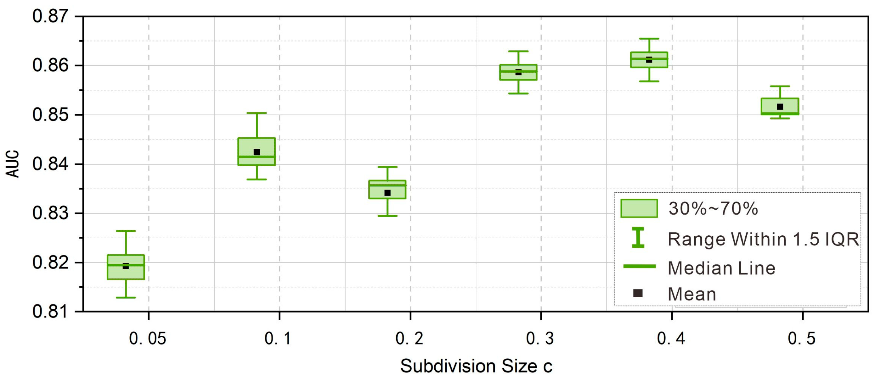
5.3.1. Accuracy Validation for Different Slope Unit Sizes

Boxplots of Area Under the Curve (AUC) values, as shown in Figure 10, were used to assess the predictive accuracy of landslide susceptibility models across varying slope unit sizes. The results revealed a scale-dependent effect, with larger slope units yielding higher predictive accuracy, while smaller units showed lower accuracy. At c = 0.4 c, the model achieved the highest accuracy, with AUC values ranging from 0.855 to 0.866 (mean = 0.859). At c = 0.3, the second-highest accuracy was observed, with AUC values ranging from 0.853 to 0.863 (mean = 0.856). The smallest scale (c = 0.05) resulted in the lowest accuracy, with AUC values ranging from 0.812 to 0.828 (mean = 0.820). These findings suggest that medium-sized slope units (c = 0.3 and c = 0.4) offer an optimal balance between spatial granularity and predictive power. In addition, Deng et al. conducted a parameter gradient experiment on 23 sets of slope units using the IV-RF model and found that a circular variance threshold of c = 0.3 resulted in the highest values for both the Area Under the ROC Curve (AUC) and the harmonic mean of precision and recall (F1) [6]. This configuration demonstrated optimal internal homogeneity and external heterogeneity, leading to the best performance in landslide susceptibility mapping.

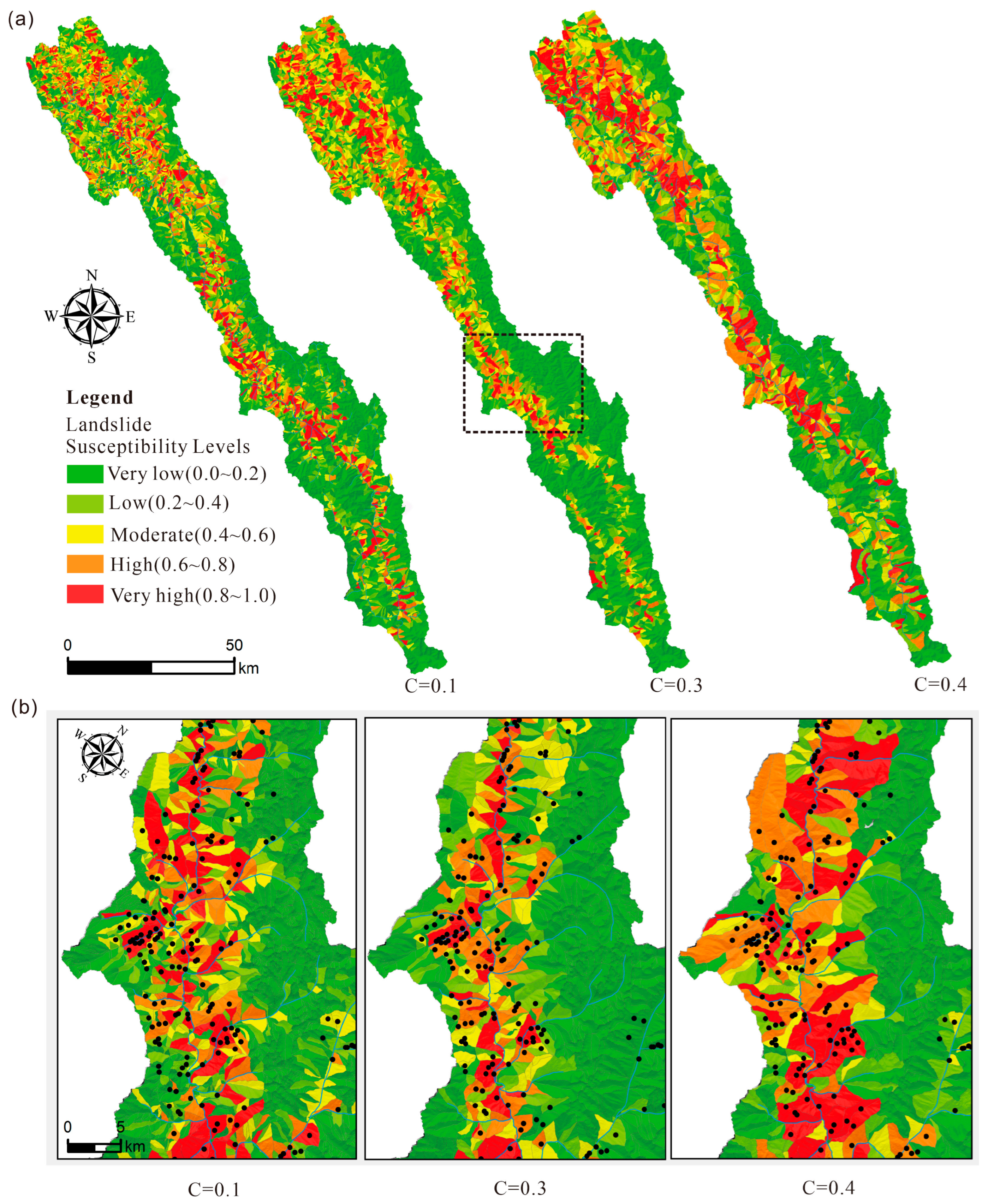
5.3.2. Zoning Results for Different Slope Unit Sizes

This study systematically evaluates the trade-off between predictive accuracy and zoning rationality in landslide susceptibility; results for slope unit sizes c = 0.1 and c = 0.4 were analyzed in detail (Figure 11). Across all scales, regions classified as “Very High” and “High Susceptibility” were concentrated in upstream areas, such as Tiatuo Town, Wangda Town, and the Zhayu section of the Yuqu River’s main channel. Conversely, “Low” and “Very Low Susceptibility” zones were predominantly located in watershed divides and downstream areas, such as Zhayu Town and Bitu Township.

Additionally, as shown in Figure 12, at c = 0.3, the Very High and High susceptibility zones covered only 8.48% of the area but captured 43.10% of historical landslides, yielding a frequency ratio of 5.06. In contrast, at c = 0.4, these zones covered 15.64% of the area and captured 39.24% of historical landslides, resulting in a lower frequency ratio of 2.51, indicating potential overestimation.

At c = 0.3, these zones covered 49.07% of the area but contained just 5.2% of historical landslides, achieving a frequency ratio of 0.10. At c = 0.1, these zones covered 53.47% of the area but included 10.52% of historical landslides, leading to a higher frequency ratio of 0.20, suggesting overgeneralization. Overall, the c = 0.3 scale provided the most balanced trade-off between predictive accuracy and zoning rationality, making it the optimal choice for landslide susceptibility evaluation in the Yuqu River Basin.

6. Discussion

6.1. Importance Analysis of Influencing Factors Across Different Slope Unit Scales

This study confirmed that landslide susceptibility zoning and predictive accuracy are strongly influenced by the scale of slope unit division. Contrary to expectations, the finest slope unit scale (c = 0.05) did not yield the highest predictive accuracy. Instead, medium and larger unit sizes improved model performance by balancing spatial heterogeneity and minimizing data noise. At the finest scale, the high sample density led to overfitting due to data redundancy and imbalanced sample proportions, making it difficult for the model to generalize predictions effectively in complex terrains. These findings align with the results of Huang et al. [10], who demonstrated that excessively fine-scale mapping can introduce data noise and obscure critical terrain features, ultimately reducing model accuracy. Similarly, Reichenbach et al. found that coarser mapping units tend to over-smooth spatial variations, leading to a loss of critical geomorphic details essential for hazard assessment [1].

As shown in Figure 13, the mean absolute SHAP values indicate that the freezing index consistently emerged as the dominant causative factor, with an importance score exceeding 0.5 across all scales. This finding aligns with previous studies that highlight the destabilizing role of freeze–thaw cycles in cold regions [33,34]. The freezing index directly affects soil cohesion and rock fracture dynamics, weakening slope stability through repeated freezing and thawing. These results are also supported by the work of Yang et al. [35] who found that freeze–thaw processes are a primary trigger for landslides in permafrost regions, particularly when interacting with topographic factors such as slope gradient and fault proximity.

Other factors, such as rainfall, lithology, slope angle, and relative height, showed variable importance rankings across different scales. For instance, at the medium scale (c = 0.3), rainfall and lithology ranked fourth and third in importance, respectively, contributing to a high mean AUC value of 0.86. However, at the larger scale (c = 0.5), the rankings of these factors decreased, resulting in a slight decline in predictive accuracy (mean AUC = 0.85). These findings suggest that extreme scales fail to adequately capture key factors, limiting the model’s predictive performance. This is consistent with the results of Schlögel et al. [36], who found that scale effects significantly influence the relative contribution of environmental variables in landslide susceptibility models, with certain factors becoming more or less significant depending on the mapping resolution used.

SHAP analysis also highlighted the scale-dependent effect on factor contributions. At the finest scale (c = 0.05), positive SHAP values of key factors were significantly weaker than their negative contributions. For instance, the positive SHAP value for the freezing index was only 0.09, while its negative contribution was 0.45. Positive SHAP values indicate a factor’s direct contribution to increasing landslide susceptibility, while negative values suggest stabilizing effects. This imbalance indicates that the model overemphasized stable zones at smaller scales, potentially overlooking key indicators of landslide-prone areas.

At larger scales (c ≥ 0.3), positive contributions became more pronounced, allowing for better differentiation between landslide-prone and stable zones. This balance reinforces the suitability of the medium scale (c = 0.3) as the optimal compromise between sample distribution uniformity and spatial heterogeneity, enabling more robust landslide risk predictions. These findings align with previous studies on scale-dependent hazard mapping, such as those by Sidle and Bogaard [3], which emphasized that integrating multi-scale analysis improves the identification of key environmental triggers and enhances prediction reliability in complex mountainous terrains.

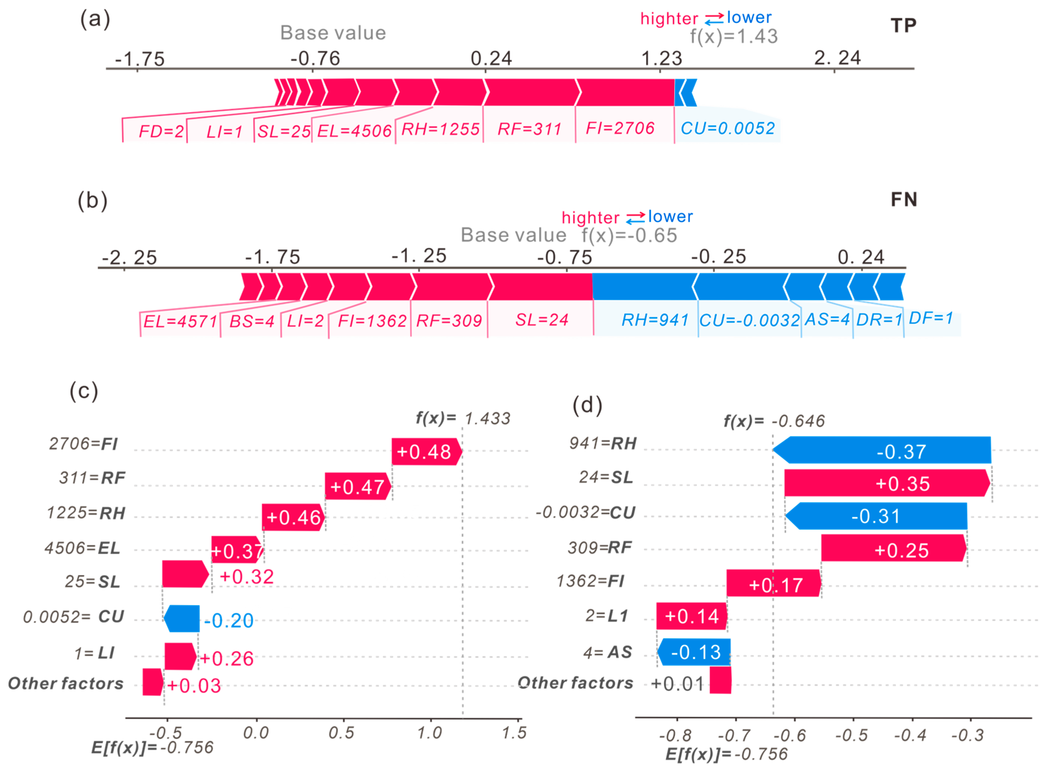
6.2. Model Interpretability Across Different Slope Unit Scales

By constructing landslide susceptibility models at multiple scales, this study revealed how slope unit size influences the contribution mechanisms of contributing factors. Smaller slope units provided abundant data samples, but the imbalance between positive and negative sample distribution and the redundancy of features led to reduced predictive accuracy and interpretability. This trend aligns with other studies that report diminished model performance with high-resolution topographic data [37]. Conversely, larger slope units oversimplified landslide characteristics due to excessive spatial smoothing, resulting in decreased performance. The medium scale (c = 0.3) demonstrated stable predictive accuracy and interpretability, underscoring its adaptability and scientific validity. As shown in Figure 14, local SHAP analysis clarified the contributions of contributing factors. For instance, at c = 0.3, freezing index, rainfall, relative height, and elevation made significant positive contributions, with average SHAP values of 0.48, 0.47, 0.46, and 0.37, respectively. These positive contributions outweighed the negative ones, underscoring the critical role of these factors in high-susceptibility zones. In contrast, finer scales (c = 0.1) amplified random noise, with factors such as curvature and aspect exhibiting increased negative contributions, thereby reducing predictive accuracy. Positive contributions at the medium scale reflected an optimal balance of feature information, minimizing noise and redundancy while preserving key factor-driven mechanisms.

These findings demonstrate that medium-scale models (c = 0.3) effectively capture the critical interplay of contributing factors, establishing this scale as a robust foundation for regional landslide prediction. Recent advancements in SHAP-based interpretability methods for geospatial models further validate the utility of medium-scale analyses in landslide susceptibility assessments [10].

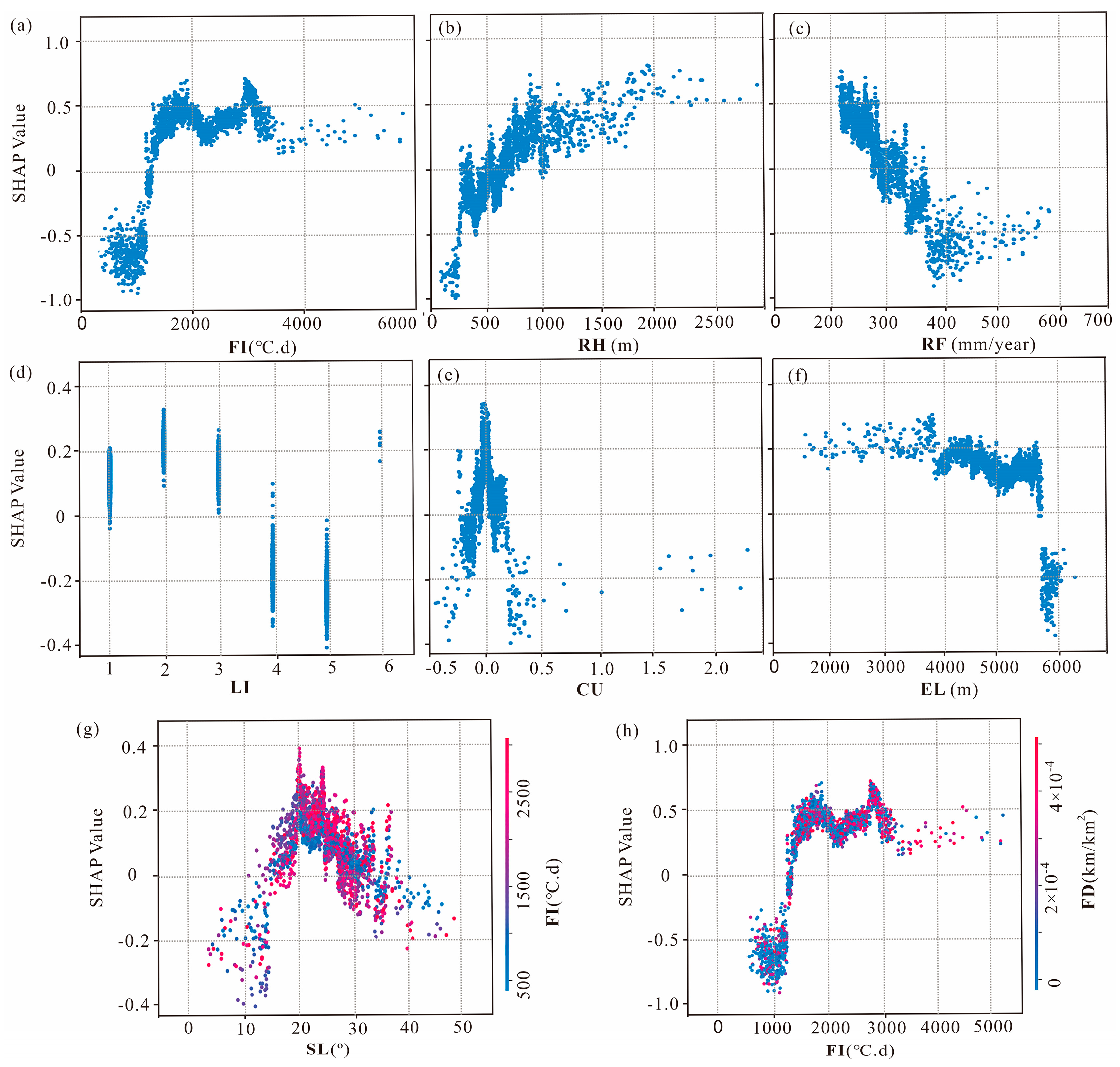
6.3. Influencing Factor Hazardous Thresholds and Synergistic Effects

While global importance rankings provide a broad overview of the influence of causative factors, understanding nonlinear response patterns and hazardous thresholds of these factors is crucial for accurate landslide predictions. Using SHAP dependence scatter plots, this study identified critical thresholds and synergistic effects for six key factors: freezing index, relative height, rainfall, lithology, curvature, and elevation.

The freezing index exhibited a nonlinear relationship, with landslide likelihood increasing sharply when the freezing index exceeded 1000 °C·d. The hazardous threshold was identified as 1500–3000 °C·d, consistent with studies on freeze–thaw thresholds in cold climates [35]. Within this range, repeated freeze–thaw cycles significantly weaken soil and rock stability, triggering landslides. Relative height showed a positive incremental response, with high landslide activity concentrated within the 500–1500 m range. This range reflects increased gravitational stress and slope instability in steep mountainous areas. Rainfall demonstrated a complex pattern. Higher rainfall regions benefited from increased vegetation cover, which stabilizes slopes. However, arid regions (200–300 mm annual rainfall) exhibited higher landslide risks due to sparse vegetation and weaker soil cohesion.

SHAP interaction analysis revealed critical interactions between factors, as shown in Figure 15g–h. Freezing index and slope gradient demonstrated strong positive interactions within the 15–25° slope range. As the freezing index increased, the contribution of slope gradient to landslide susceptibility intensified, highlighting the combined effects of reduced cohesion and gravitational stress. Freezing index and fault density also exhibited compounding effects. For instance, areas with a freezing index of 2700–2900 °C·d and higher fault density experienced elevated landslide probabilities. Fault zones amplify slope instability by weakening rock mass integrity, which is further exacerbated by freeze–thaw cycles.

These findings highlight the importance of incorporating both individual factor thresholds and multi-factor interactions into landslide susceptibility models. Factors such as freezing index, relative height, and rainfall not only have significant individual impacts but also amplify their effects through synergistic interactions under specific environmental conditions. Similar interactions between geological and climatic factors have been observed in other regional susceptibility studies [3]. Understanding these interactions provides valuable insights into the complex mechanisms driving landslide susceptibility in mountainous terrains, guiding future efforts to refine predictive models.

7. Conclusions

This study systematically examined the impact of slope unit division scales on landslide susceptibility assessment (LSA) in the Yuqu River Basin, utilizing SHAP to enhance model transparency. It addressed key gaps in standardized slope unit strategies and the application of interpretable machine learning techniques for LSA. The findings highlight the significant impact of slope unit scale on sample size, spatial feature distribution, and predictive performance.

At the smallest scale (c = 0.05), the high density of samples introduced data redundancy and imbalances, reducing the model’s effectiveness in identifying landslide-prone areas. Conversely, at the largest scale (c = 0.5), excessive smoothing of spatial features obscured critical heterogeneity, resulting in lower predictive accuracy. The medium scale (c = 0.3) emerged as the optimal choice, balancing spatial heterogeneity and uniform sample distribution. This scale minimized data noise while effectively capturing critical environmental features, achieving near-maximum predictive accuracy (mean AUC = 0.856). Key contributing factors, including freezing index, relative height, and rainfall, were identified with distinct hazardous thresholds. For example, freezing index values between 1500 and 3000 °C·d and relative heights of 500–1500 m significantly increased landslide susceptibility. Freeze–thaw cycles weaken slope stability, while elevated terrains amplify gravitational stress, triggering slope failures. Synergistic interactions further intensified landslide risks, particularly the combined effects of freezing index with slope gradient (15–25°) and fault density in high-value ranges (2700–2900 °C·d). By integrating SHAP, this study enhanced the interpretability of machine learning models, addressing the “black-box” challenge in LSA.

Nevertheless, this study has certain limitations that warrant further investigation. First, the landslide inventory and environmental datasets primarily originate from the Yuqu River Basin, which may constrain the generalizability of the proposed framework to regions with distinct geological or climatic conditions. For example, Belair [38] developed and evaluated the generalizability of regional landslide susceptibility models across different areas. Second, the static nature of the input data (e.g., historical landslide records and fixed climatic indices) fails to account for temporal variations, such as long-term climate change and evolving anthropogenic influences, which could significantly reshape landslide susceptibility patterns. Third, while SHAP provides valuable insights into factor contributions, its capacity to elucidate complex nonlinear interactions among variables remains constrained by the model’s inherent assumptions.

Future research should seek to address these limitations. First, validating the framework across diverse geographical contexts (e.g., arid or coastal regions) would enhance its robustness and applicability. Second, integrating time-series data, such as real-time rainfall monitoring and seismic activity records, could improve the model’s ability to capture dynamic landslide triggers. Third, exploring hybrid approaches that combine XGBoost with deep learning architectures may further enhance predictive performance while maintaining interpretability. For example, Li [39] employed time-series InSAR technology to obtain surface deformation data and integrated deep learning to develop an LSTM-TCN displacement prediction model for studying landslide displacement forecasting. Lastly, conducting multi-scale analyses that incorporate slope units alongside grid-based or administrative divisions could not only enhance the understanding of landslide mechanisms across varying spatial resolutions, but also provide valuable insights for developing region-specific landslide risk management strategies and informing evidence-based policy decisions.

References

1. Reichenbach, P.; Rossi, M.; Malamud, B.D.; Mihir, M.; Guzzetti, F. A review of statistically-based landslide susceptibility models. Earth-Sci. Rev. 2018, 180, 60–91. [Google Scholar] [CrossRef]
2. Bammou, Y.; Benzougagh, B.; Ouallali, A.; Kader, S.; Raougua, M.; Igmoullan, B. Improving landslide susceptibility mapping in semi-arid regions using machine learning and geospatial techniques. DYSONA—Appl. Sci. 2025, 6, 269–290. [Google Scholar]
3. Sidle, R.C.; Bogaard, T.A. Dynamic earth system and ecological controls of rainfall-initiated landslides. Earth-Sci. Rev. 2016, 159, 275–291. [Google Scholar] [CrossRef]
4. Iida, T. A stochastic hydro-geomorphological model for shallow landsliding due to rainstorm. CATENA 1999, 34, 293–313. [Google Scholar] [CrossRef]
5. Luo, W.; Liu, C.C. Innovative landslide susceptibility mapping supported by geomorphon and geographical detector methods. Landslides 2018, 15, 465–474. [Google Scholar] [CrossRef]
6. Deng, H.; Wu, X.T.; Zhang, W.J.; Liu, Y.S.; Li, W.L.; Li, X.Y.; Zhou, P.; Zhuo, W.Z. Slope-Unit Scale Landslide Susceptibility Mapping Based on the Random Forest Model in Deep Valley Areas. Remote Sens. 2022, 14, 4245. [Google Scholar] [CrossRef]
7. Chen, T.Q.; Guestrin, C. XGBoost: A Scalable Tree Boosting System. In Proceedings of the 22nd ACM SIGKDD International Conference on Knowledge Discovery and Data Mining, San Francisco, CA, USA, 13–17 August 2016; pp. 785–794. [Google Scholar]
8. Sahin, E.K. Assessing the predictive capability of ensemble tree methods for landslide susceptibility mapping using XGBoost, gradient boosting machine, and random forest. SN Appl. Sci. 2020, 2, 1308. [Google Scholar] [CrossRef]
9. Zhang, J.Y.; Ma, X.L.; Zhang, J.L.; Sun, D.L.; Zhou, X.Z.; Mi, C.L.; Wen, H.J. Insights into geospatial heterogeneity of landslide susceptibility based on the SHAP-XGBoost model. J. Environ. Manag. 2023, 332, 117357. [Google Scholar] [CrossRef]
10. Huang, F.M.; Cao, Y.; Li, W.B.; Catani, F.; Song, G.Q.; Huang, J.S.; Yu, C.S. Uncertainties of landslide susceptibility prediction: Influences of different study area scales and mapping unit scales. Int. J. Coal Sci. Technol. 2024, 11, 26. [Google Scholar] [CrossRef]
11. Crozier, M.J. Landslide geomorphology: An argument for recognition, with examples from New Zealand. Geomorphology 2010, 120, 3–15. [Google Scholar] [CrossRef]
12. Gong, Y.F.; Yao, A.J.; Li, Y.L.; Li, Y.Y.; Tian, T. Classification and distribution of large-scale high-position landslides in southeastern edge of the Qinghai-Tibet Plateau, China. Environ. Earth Sci. 2022, 81, 311. [Google Scholar] [CrossRef]
13. Korup, O. Geomorphic implications of fault zone weakening: Slope instability along the Alpine Fault, South Westland to Fiordland. N. Z. J. Geol. Geophys. 2004, 47, 257–267. [Google Scholar] [CrossRef]
14. Xu, C.; Xu, X.W.; Shyu, J.B.H. Database and spatial distribution of landslides triggered by the Lushan, China Mw 6.6 earthquake of 20 April 2013. Geomorphology 2015, 248, 77–92. [Google Scholar] [CrossRef]
15. Zhao, B.; Wang, Y.S.; Li, W.L.; Su, L.J.; Lu, J.Y.; Zeng, L.; Li, X. Insights into the geohazards triggered by the 2017 Ms 6.9 Nyingchi earthquake in the east Himalayan syntaxis, China. CATENA 2021, 205, 105467. [Google Scholar] [CrossRef]
16. Xu, X.W.; Wen, X.Z.; Zheng, R.Z.; Ma, W.T.; Song, F.M.; Yu, G.H. Pattern of latest tectonic motion and its dynamics for active blocks in Sichuan-Yunnan region, China. Sci. China Ser. D Earth Sci. 2003, 46, 210–226. [Google Scholar] [CrossRef]
17. Guzzetti, F.; Galli, M.; Reichenbach, P.; Ardizzone, F.; Cardinali, M. Landslide hazard assessment in the Collazzone area, Umbria, Central Italy. Nat. Hazards Earth Syst. Sci. 2006, 6, 115–131. [Google Scholar] [CrossRef]
18. Yang, J.H.; Wu, G.L.; Jiao, J.Y.; Dyck, M.; He, H.L. Freeze-thaw induced landslides on grasslands in cold regions. CATENA 2022, 219, 106650. [Google Scholar] [CrossRef]
19. Tsou, C.Y.; Chigira, M.; Matsushi, Y.; Hiraishi, N.; Arai, N. Coupling fluvial processes and landslide distribution toward geomorphological hazard assessment: A case study in a transient landscape in Japan. Landslides 2017, 14, 1901–1914. [Google Scholar] [CrossRef]
20. Zou, Y.; Qi, S.W.; Guo, S.F.; Zheng, B.W.; Zhan, Z.F.; He, N.W.; Huang, X.L.; Hou, X.K.; Liu, H.Y. Factors controlling the spatial distribution of coseismic landslides triggered by the Mw 6.1 Ludian earthquake in China. Eng. Geol. 2022, 296, 106477. [Google Scholar] [CrossRef]
21. Guo, F.F.; Yang, N.; Meng, H.; Zhang, Y.Q.; Ye, B.Y. Application of the Relief Amplitude and Slope Analysis to Regional Landslide Hazard Assessments. Geol. China 2008, 35, 131–143. [Google Scholar]
22. Guo, C.B.; Montgomery, D.R.; Zhang, Y.S.; Wang, K.; Yang, Z.H. Quantitative assessment of landslide susceptibility along the Xianshuihe fault zone, Tibetan Plateau, China. Geomorphology 2015, 248, 93–110. [Google Scholar] [CrossRef]
23. Wang, Y.H.; Wang, L.Q.; Liu, S.L.; Liu, P.F.; Zhu, Z.W.; Zhang, W.G. A comparative study of regional landslide susceptibility mapping with multiple machine learning models. Geol. J. 2024, 59, 2383–2400. [Google Scholar] [CrossRef]
24. Ma, J.W.; Wang, Y.K.; Niu, X.X.; Jiang, S.; Liu, Z.Y. A comparative study of mutual information-based input variable selection strategies for the displacement prediction of seepage-driven landslides using optimized support vector regression. Stoch. Environ. Res. Risk Assess. 2022, 36, 3109–3129. [Google Scholar] [CrossRef]
25. Sun, H.Q.; Li, W.Y.; Scaioni, M.; Fu, J.; Guo, X.; Gao, J. Influence of spatial heterogeneity on landslide susceptibility in the transboundary area of the Himalayas. Geomorphology 2023, 433, 108723. [Google Scholar] [CrossRef]
26. Alvioli, M.; Marchesini, I.; Reichenbach, P.; Rossi, M.; Ardizzone, F.; Fiorucci, F.; Guzzetti, F. Automatic delineation of geomorphological slope units with r.slopeunits v1.0 and their optimization for landslide susceptibility modeling. Geosci. Model. Dev. 2016, 9, 3975–3991. [Google Scholar] [CrossRef]
27. Probst, P.; Wright, M.N.; Boulesteix, A.L. Hyperparameters and tuning strategies for random forest. Wiley Interdiscip. Rev. Data Min. Knowl. Discov. 2019, 9, e1301. [Google Scholar] [CrossRef]
28. Friedman, J.H. Stochastic gradient boosting. Comput. Stat. Data. Anal. 2022, 38, 367–378. [Google Scholar] [CrossRef]
29. Kuhn, M.; Johnson, K. Applied Predictive Modeling; Springer: New York, NY, USA, 2013; Volume 26, p. 13. [Google Scholar]
30. Brenning, A. Spatial prediction models for landslide hazards: Review, comparison and evaluation. Nat. Hazards Earth Syst. Sci. 2005, 5, 853–862. [Google Scholar] [CrossRef]
31. Nath, R.R.; Pal, S.; Sharma, M.L. Use of Probabilistically Generated Scenario Earthquakes in Landslide Hazard Zonation: A Semi-Qualitative Approach; Springer: Singapore, 2022; pp. 247–274. [Google Scholar]
32. Tsangaratos, P.; Ilia, I.; Hong, H.Y.; Chen, W.; Xu, C. Applying Information Theory and GIS-based quantitative methods to produce landslide susceptibility maps in Nancheng County, China. Landslides 2017, 14, 1091–1111. [Google Scholar] [CrossRef]
33. Li, J.L.; Zhou, K.P.; Liu, W.J.; Zhang, Y.M. Analysis of the effect of freeze–thaw cycles on the degradation of mechanical parameters and slope stability. Bull. Eng. Geol. Environ. 2018, 77, 573–580. [Google Scholar] [CrossRef]
34. Li, T.Z.; Zhang, L.M.; Gong, W.P.; Tang, H.M.; Jiang, R.C. Initiation mechanism of landslides in cold regions: Role of freeze-thaw cycles. Int. J. Rock Mech. Min. Sci. 2024, 183, 105906. [Google Scholar] [CrossRef]
35. Yang, Z.Z.; Ni, W.K.; Niu, F.J.; Li, L.; Ren, S.Y. Spatiotemporal Distribution Characteristics and Influencing Factors of Freeze-Thaw Erosion in the Qinghai-Tibet Plateau. Remote Sens. 2024, 16, 1629. [Google Scholar] [CrossRef]
36. Schlögel, R.; Marchesini, I.; Alvioli, M.; Reichenbach, P.; Rossi, M.; Malet, J.P. Optimizing landslide susceptibility zonation: Effects of DEM spatial resolution and slope unit delineation on logistic regression models. Geomorphology 2018, 301, 10–20. [Google Scholar] [CrossRef]
37. Lu, Z.Y.; Liu, G.Y.; Song, Z.H.; Sun, K.; Li, M.; Chen, Y.S.; Zhao, X.D.; Zhang, W. Advancements in Technologies and Methodologies of Machine Learning in Landslide Susceptibility Research: Current Trends and Future Directions. Appl. Sci. 2024, 14, 9639. [Google Scholar] [CrossRef]
38. Belair, G.; Bendick, R. Development of Regional Landslide Susceptibility Models: A First Step Towards Model Transferability. Geol. Soc. Am. 2022, 54, 5. [Google Scholar]
39. Li, J.; Fan, C.P.; Zhao, K.; Zhang, Z.; Duan, P. Landslide displacement prediction using time series InSAR with combined LSTM and TCN: Application to the Xiao Andong landslide, Yunnan Province, China. Nat. Hazards 2025, 121, 3857–3884. [Google Scholar] [CrossRef]
Figure 1. Geographical context of the Yuqu River Basin, southeastern Tibet: (a) Geographic location; (b) Elevation ranges and key geomorphological zones.
Water 17 01877 g001
Figure 2. Spatial distribution and morphological diversity of historical landslides in the Yuqu River Basin (2014–2020), red dotted frame: Geographic location of landslide; yellow dotted: landslide boundary: (a) Macro distribution of 1329 landslide events; (bd) Representative examples of landslide morphology.
Water 17 01877 g002
Figure 3. Spatial variability of key landslide contributing factors in the Yuqu River Basin: (a) Elevation; (b) Relative height; (c) Slope; (d) Aspect; (e) Curvature; (f) Lithology; (g) Fault density; (h) Distance to faults; (i) Bank slope; (j) River density; (k) Distance to rivers; (l) Terrain wetness index; (m) PGA; (n) Rainfall; (o) Freezing index.
Water 17 01877 g003
Figure 4. Methodological workflow for multi-scale landslide susceptibility assessment: From data preprocessing to SHAP-based interpretability.
Water 17 01877 g004
Figure 5. Schematic representation of the XGBoost Ensemble Learning Framework for landslide susceptibility prediction.
Water 17 01877 g005
Figure 6. Interpretable SHAP model for landslide susceptibility: Global feature importance and local decision contributions.
Water 17 01877 g006
Figure 7. Comparative analysis of slope unit sizes (c = 0.05–0.5) in the Yuqu River Basin: Spatial heterogeneity and unit morphology: As the slope unit size increases (af), the total number of samples gradually decreases, while the ratio of landslide samples to non-landslide samples gradually increases.
Water 17 01877 g007
Figure 8. Global functional values of slope unit groups: (a) OCE values; (b) GS values of slope unit groups when OCE < 0.35; (c) GS values calculated from all 30 slope unit groups.
Water 17 01877 g008
Figure 9. Mutual information analysis between landslide occurrence and contributing factors across slope unit scales (c = 0.05–0.5).
Water 17 01877 g009
Figure 10. Model performance comparison (AUC Values) across six slope unit scales (c = 0.05–0.5): Boxplots of 20 repeated validations.
Water 17 01877 g010
Figure 11. Landslide susceptibility zonation based on centroid points at different slope unit scales (c = 0.1, c = 0.3, c = 0.4): (a) Overview of the Yuqu River Basin; (b) Local detail within the Yuqu River Basin.
Water 17 01877 g011
Figure 12. Statistical analysis of landslide susceptibility zoning across different slope unit scales: (a) Landslide susceptibility index distribution; (b) Proportion of area by susceptibility zones.
Water 17 01877 g012
Figure 13. The rankings of causative factor importance for different slope unit scales: (a) Fine scale (c = 0.05); (b) Intermediate fine scale (c = 0.1); (c) Medium scale (c = 0.3); (d) Large scale (c = 0.5).
Water 17 01877 g013
Figure 14. Local predictions interpreted using SHAP at different scales: (a,b) Local interpretation force plots for true positives (TP) and false negatives (FN); (c,d) Corresponding waterfall plots illustrating the contribution of each factor for TP and FN samples.
Water 17 01877 g014
Figure 15. Nonlinear responses and synergistic effects of key conditioning factors on landslide susceptibility based on SHAP analysis: (af) illustrate the nonlinear relationships between six key conditioning factors—freezing index, relative relief, rainfall, lithological group, curvature, and elevation—and their SHAP values, indicating the marginal contribution of each variable to landslide susceptibility; (g,h) illustrate the interactive effects of the freezing index with slope (g), and with fault density (h).
Water 17 01877 g015