Experimental and Numerical Analysis of Evaporation Processes in a Semi-Arid Region

Abstract

This study combines field experiments and numerical analysis using the HYDRUS model to investigate the impact of water table depths on evaporation processes in semi-arid regions with shallow groundwater. Two lysimeters with different water table depths were set up in the Ordos Basin, Northwest China, and instrumented with multi-depth soil moisture and temperature sensors. The experimental data were used to calibrate and validate numerical models that simulated both non-isothermal and isothermal flows. The results reveal that groundwater levels significantly influence the evaporation rate, dictating the position of the evaporation front and zero-flux plane. Isothermal models underestimated cumulative evaporation by 14.7% and 44.2% for the shallow and deep-water table lysimeters, respectively, while non-isothermal models produced more accurate results with 0.95% overestimation and 5.2% underestimation. The study demonstrates that incorporating both water and heat transport into numerical models enhances the accuracy of evaporation estimates under varying groundwater conditions. Furthermore, the findings show that when the evaporation front occurs near the surface, liquid water flux dominates, whereas water vapor flux plays a crucial role when the evaporation front is located below the surface. These results offer valuable insights for refining water management strategies and models in agricultural and ecological systems of semi-arid areas, underscoring the critical role of considering soil moisture and temperature dynamics, along with groundwater levels, in accurately quantifying evaporation for improved resource management.

1. Introduction

The average global evapotranspiration (ET) from the Earth’s terrestrial surface accounts for about two-thirds of the average global precipitation [1] Bare soil evaporation is a critical component of ET, representing a significant portion of the water cycle in various ecosystems. Understanding bare soil evaporation is particularly critical in the context of global climate change and water resource management [2]. As global temperatures rise and water scarcity become more pronounced [3], particularly in arid and semi-arid regions, the dynamics of soil evaporation are expected to shift, potentially exacerbating water stress and land degradation [4]. This has direct implications for agricultural productivity, ecosystem health, and the sustainability of water resources. Therefore, improving our understanding of bare soil evaporation is not only a scientific priority [5] but also a practical necessity for addressing global environmental challenges.

Although research of soil evaporation has spanned over a century, our understanding of the dynamic mechanisms involved in evaporation from porous media remains incomplete [6]. This is partly due to the complexity of the process, which involves multiphase interactions, mass transfer, pore-scale energy dynamics, and phase change [7]. Several factors influence soil evaporation, including soil moisture, soil heterogeneity, shallow water table depth, soil hydraulic and thermal properties, and atmospheric conditions [8]. Among these, the shallow water table has a particularly straightforward effect on soil evaporation. Early theoretical work by Veihmeyer and Brooks [9], Gardner and Fireman [10], and Shih [11] suggested that water table depth significantly affects bare soil evaporation. For example, Veihmeyer and Brooks [9] found that evaporation rates decreased significantly when the water table was lowered to a certain depth, and the relationship between evaporation rate and water table depth was not linear. Hellwig [12] further demonstrated that lowering the water table depth to 60 cm below the surface reduced the evaporation rate to 10% of that from an open-water surface. Shih [11] also pointed out that increasing the water table depth could effectively reduce evaporation loss from the soil surface. However, these studies often neglected the effect of soil temperature on evaporation, and many analytical solutions [13,14] derived to calculate evaporation rates assumed a hydraulic connection between the surface and the water table, which may not always be valid [15].

Recent advancements in soil–atmosphere interaction modeling have provided new insights into the complexities of evaporation processes. For instance, data-driven approaches [16] have emerged as powerful tools for estimating evaporation, particularly in heterogeneous and dynamic environments. Studies such as those by Yonaba, et al. [17] and Eshetu, et al. [18] have demonstrated the effectiveness of machine learning and remote sensing techniques in improving the accuracy of capturing the nonlinear relationships between soil properties, atmospheric conditions, and evaporation rates, offering a more comprehensive understanding of the process. To improve the mechanistic understanding of bare soil evaporation in the presence of a shallow water table, many laboratory experiments have been conducted. Rose, et al. [19] and Gowing, et al. [20] compared the effects of different water table depths on soil evaporation using pseudo steady-state models, neglecting soil temperature effects. They found that the depth of the evaporation front (the interface between wet and dry zones) could be a criterion for preventing salinization due to capillary flow from shallow water tables in arid regions. Wang, et al. [21] conducted laboratory experiments and numerical modeling to investigate water movement and heat transport in the unsaturated zone, finding that the maximum depth for phreatic water to contribute to soil evaporation was approximately 70 cm for silt and fine sand. They also emphasized the importance of accounting for nonisothermal processes in arid and semi-arid regions where ground temperatures exceed 25 °C. Shokri and Salvucci [15] demonstrated the limitations of assuming liquid continuity (capillary flow continuity) through the vadose zone over large distances above a water table, showing that evaporation rates were significantly suppressed when the water table depth exceeded the maximum depth for hydraulic connection to the surface.

In contrast to controlled laboratory experiments, in situ experiments are more complex due to temporal variations in precipitation, net radiation, and water table depth [22]. The cost of equipment and operation also limits field experiments [23]. However, understanding evaporation processes under natural conditions is crucial for environmental management, particularly in addressing bioenvironmental issues such as desertification [24]. Many current models fail to couple evaporation with energy and mass transfer processes under the bare ground condition due to the complexity of field settings and a lack of field data [8]. Therefore, there is an urgent need to explore evaporation processes under natural conditions, especially in the presence of a shallow water table, to improve our understanding and inform sustainable water management practices globally.

This study aims to address these gaps by improving the understanding of evaporation processes from bare ground in the presence of a shallow water table. We hypothesize that the depth of the shallow water table significantly influences soil evaporation rates under natural conditions and that non-isothermal processes play a critical role in arid and semi-arid regions. To test this hypothesis, we conducted two in situ lysimeter experiments in the semi-arid Ordos Basin, Northwest China, under natural weather conditions but with different initial water table depths. Unlike other methods such as remote sensing or eddy covariance, lysimeters allow for the direct measurement of water loss from the soil surface, making them particularly suitable for studying the effects of shallow water tables on evaporation. The experiments were instrumented with multi-depth soil moisture sensors and groundwater depth sensors, recording high-resolution data over four months (July to October 2015). Two models were constructed to simulate both non-isothermal and isothermal flows in the lysimeters, allowing us to infer the effects of the shallow water table on soil evaporation under natural conditions. By addressing these research gaps, this study contributes to international efforts to better understand and manage water resources in arid and semi-arid regions where water scarcity and land degradation are pressing concerns. The findings are expected to benefit policymakers, environmental managers, and researchers working on sustainable land and water management strategies globally.

2. Materials and Methods

This study is based on the Mu Us Sandy Land, China (Figure 1). The region is a semi-arid shrubland ecosystem characterized by sparse vegetation a relatively flat terrain, covering an area of approximately 40,000 km² [25]. The region experiences a continental semi-arid climate, with a mean annual precipitation of 340 mm and a mean annual potential evapotranspiration of 2180 mm [26]. The dryness index (evaporation divided by precipitation) is 6.7, highlighting the region’s aridity. Groundwater level in this region ranges from 0.4 to 15 m below the land surface, and groundwater evaporation contributes significantly to the water balance, accounting for 53–56% of total ET during the dry season [27]. These characteristics make the Mu Us Sandy Land an ideal area for investigating evaporation processes in the presence of shallow water table.

Precipitation in the region is episodic and sometimes intense, with significant seasonal variability. From 1 July 2015 to 30 June 2016, a total of 54 precipitation events were recorded, predominantly occurring during summer and autumn months (Figure 2). Individual precipitation events ranged from 0.1 and 40 mm, with a cumulative annual total of 270.1 mm. Seasonal trends in potential ET also exhibit variability, with higher rates during the warmer months (June–August) and lower rates during the colder months (December–February).

Air temperature in the region fluctuates strongly over short periods but follows a clear seasonal pattern. During the study period, the maximum air temperature of 28.1 °C was recorded in August 2015, while the minimum temperature of −26.8 °C occurred in February 2016 (Figure 2). The annual mean air temperature was 4.3 °C, reflecting the region’s cold winters and relatively mild summers. These climatic conditions, combined with the shallow groundwater table, create a dynamic environment for studying evaporation and water balance processes in semi-arid ecosystems.

2.1. Lysimeters

We built two lysimeters at the Henan Country national weather station in Northwest China (Figure 3). The two lysimeters had the same diameter of 2 m but different depths (1.2 and 4.2 m). They were first buried in the soil with the top outcropping at the land surface as shown in Figure 3 and then packed with local sandy soil. Afterwards, they were filled with fresh water until their water levels reached 1 and 2 m below the surface ground, respectively. To ensure the accuracy of the final water levels, the water was added slowly with an increment of 10 cm and allowed to settle for 1 h before the next increment.

2.2. Date Collection

Our experiment was performed from 1 July to 13 October 2015. The lysimeters were instrumented with several sensors with ±1~2% accuracy (ECH2O-5TM, Decagon Inc., Washington, DC, USA) to measure soil moisture and temperature (Figure 3). In lysimeter 1, the sensors were placed at the depths of 3, 10, 20, 30, 50, and 80 cm below the surface ground, whereas in lysimeter 2, they were installed at the depths of 10, 20, 30, 50, 80, 150, 250, and 350 cm below surface ground. Due to the significant variations in soil moisture and temperature near the surface ground, the sensors are meticulously arranged in relatively dense configurations. All the sensors were connected to data loggers (Campbell CR3000, South Salt Lake City, UT, USA), and data were logged with a time interval of 5 min. Groundwater depth was measured using sensor-DI501 with an accuracy of ±0.05% (Diver, Van Essen Instruments, Delft, The Netherlands) in both lysimeters. Data were also recorded with a time interval of 5 min. At the same time, air pressure was also monitored using another sensor-DI501 in order to correct the measured groundwater level. Meteorological variables including precipitation, relative humidity, air temperature, wind speed/direction, and net radiation in the experimental site were monitored with an automatic weather station. These data were logged with hourly intervals.

2.3. Soil Hydraulic Properties

The soil used in this study consists of approximately 97.5% sand, 2.5% silt and 0% clay with in situ dry bulk density of 1.55 g/cm³. The retention curve parameters of the soil were estimated in the lab through two steps including measuring moisture contents at different matric potentials using Ku-pF apparatus (UGT GmbH, Muncheberg, Germany) and fitting the data with the van Genuchten retention curve model [30]. The saturated hydraulic conductivity was measured through field experiments using a double-ring infiltrometer based on Lai and Ren [31]. All the obtained parameters are listed in

Table 1. The van Genuchten retention curve parameters and saturated hydraulic conductivity [29].

${\mathit{\theta }}_{\mathit{r}}$ (cm3/cm3)	${\mathit{\theta }}_{\mathit{s}}$ (cm3/cm3)	$\mathit{\alpha }$ (cm−1)	$\mathit{n}$ (-)	${\mathit{K}}_{\mathit{s}}$ (cm/h)
0.015	0.31	0.020	4.84	4.6

.

3. Numerical Modeling

3.1. Model Description

The numerical code HYDRUS-1D [32] was employed in this study to simulate both dual-phase flow and heat transport simultaneously in the vertical direction. The governing equation of the dual-phase flow is given by Saito, et al. [33]:

$${\displaystyle \frac{\partial ({\theta }_L+{\theta }_v)}{\partial t}}=-{\displaystyle \frac{\partial q_L}{\partial z}}-{\displaystyle \frac{\partial q_v}{\partial z}}$$

(1)

where $q_L$ and $q_v$ represent the flux densities of the liquid water and water vapor (cm/h), respectively; ${\theta }_L$ and ${\theta }_v$ are the volumetric liquid water content and the volumetric water vapor content (cm³/cm³), respectively; $t$ is the time (h); and $z$ is the vertical distance from the datum with positive upward (cm).

The liquid water flux density $q_L$ is given by Saito, et al. [33]:

$$q_L=q_{Lh}+q_{LT}=-K_{Lh}{\displaystyle \left({\displaystyle \frac{\partial h}{\partial z}}+1\right)}-K_{LT}({\displaystyle \frac{\partial T}{\partial z}})$$

(2)

where $q_{Lh}$ and $q_{LT}$ are the isothermal and thermal liquid water flux densities (cm/h), respectively; $h$ is the pressure head (cm); $T$ is the soil temperature (°C); $K_{Lh}$ (cm/h) and $K_{LT}$ (cm²/°C/h) are the isothermal and thermal hydraulic conductivities for the liquid-phase fluxes due to the gradients of $h$ and $T$, respectively. $K_{Lh}$ and ${\theta }_L$ are nonlinear functions of $h$. Their relationships are described using the widely used van Genuchten soil water retention model, which requires five parameters including residual moisture content ${\theta }_r$ (cm³/cm³), saturated moisture content ${\theta }_s$(cm³/cm³), a soil pore-size distribution parameter $\alpha$ (1/cm), a function of the pore size distribution $n$ (-), and the saturated hydraulic conductivity of soil $K_s$ (cm/h). $K_{LT}$ is a function of $K_{Lh}$, $h$, and $T$ and so computed internally by HYDRUS-1D.

The water vapor flux density $q_v$ is written as follows [33]:

$$q_v=q_{vh}+q_{vT}=-K_{vh}({\displaystyle \frac{\partial h}{\partial z}}+1)-K_{vT}{\displaystyle \frac{\partial T}{\partial z}}$$

(3)

where $q_{vh}$ and $q_{vT}$ are the isothermal and thermal water vapor flux densities (cm/h), respectively; $K_{vh}$ (cm/h) and $K_{vT}$ (cm²/°C/h) are the isothermal and thermal vapor hydraulic conductivities, respectively. Both $K_{vh}$ and $K_{vT}$ are functions of several time-varying variables including vapor diffusivity in soil, saturated vapor density, relative humidity, and soil temperature. As the variables are dependent on either model output (soil temperature) or field observation (air temperature), both $K_{vh}$ and $K_{vT}$ are calculated along with model simulations internally.

Heat transport is solved simultaneously to provide temperature distribution in the vertical profile. The heat transport governing equation that accounts for the effects of water vapor diffusion can be written as follows [33]:

$$C_p({\theta }_L){\displaystyle \frac{\partial T}{\partial t}}+L_o{\displaystyle \frac{\partial {\theta }_v}{\partial t}}={\displaystyle \frac{\partial }{\partial z}}\left(\lambda ({\theta }_L){\displaystyle \frac{\partial T}{\partial z}}\right)-C_w{q}_L{\displaystyle \frac{\partial T}{\partial z}}-C_v{\displaystyle \frac{\partial \left(q_{v}T\right)}{\partial z}}-L_o{\displaystyle \frac{\partial q_v}{\partial z}}$$

(4)

where $C_p\left({\theta }_L\right)$, $C_w,$ and $C_v$ are the volumetric heat capacity (J/cm³/°C) of the porous medium, liquid water, and water vapor, respectively; $L_o$ is the volumetric latent heat of vaporization of liquid water (J/cm³), computed internally as a function of air temperature; $\lambda \left({\theta }_L\right)$ is the thermal conductivity of the porous medium (J/°C/cm/h). $C_p\left({\theta }_L\right)$ is dependent on time-varying ${\theta }_L$ and is calculated internally.

The thermal conductivity $\lambda \left({\theta }_L\right)$ can be described by Marsily [34]:

$$\lambda \left({\theta }_L\right)={\lambda }_0\left({\theta }_L\right)+{\beta }_t{C}_w\left|q\right|$$

(5)

where ${\beta }_t$ is the thermal dispersivity (cm); ${\lambda }_0\left({\theta }_L\right)$ is the baseline thermal conductivity, defined by Chung and Horton [35]:

$${\lambda }_0=b_1+b_2{\theta }_L+b_3{{\theta }_L}^{0.5}$$

(6)

where $b_1$, $b_2,$ and $b_3$ are empirical parameters (W/cm/°C).

3.2. Model Setup

One-dimensional models were constructed to perform numerical simulations. The heights of the models were 120 and 420 cm for lysimeters 1 and 2, respectively. Both models were discretized with a constant elemental size of 1 cm. The discretization resulted in 121 and 421 nodes for the two models, respectively. Proper initial conditions are required to simulate dual-phase flow and heat transport correctly. For dual-phase flow, either pressure head or moisture content can be accepted as the initial condition. In each model, we linearly interpolated the moisture content measured at various depths on 1 July 2015 to the entire profile and used the interpolated moisture content distribution as the dual-phase flow initial condition. Similarly, we interpolated the soil temperature measured on 1 July 2015 to the entire profile in the linear manner and treated the temperature distribution as the initial condition of the heat transport.

In each model, we specified the top boundary with an atmospheric boundary condition, which consists of several time-varying variables including net radiation, precipitation, air temperature, relative humidity, and wind speed. These time-varying variables were used to compute the evaporation rates and ground-heat fluxes required as direct boundary conditions for solving the governing equations of the dual-phase flow and heat transport. The bottom boundary of each model was assigned time-varying pressure head and temperature for simulating the dual-phase flow and the heat transport, respectively.

The models were divided into four and three layers for lysimeters 1 and 2, respectively (

Table 2. Calibrated hydraulic and thermal parameters used in the numerical model of lysimeter 1.

Lysimeter 1	Hydraulic Parameters					Thermal Conductivity
Soil Depths (cm)	${\mathit{\theta }}_{\mathit{r}}$	${\mathit{\theta }}_{\mathit{s}}$	$\mathit{\alpha }$	$\mathit{n}$	${\mathit{K}}_{\mathit{s}}$	${\mathit{b}}_1$	${\mathit{b}}_2$	${\mathit{b}}_3$
	(cm3/cm3)	(cm3/cm3)	(cm−1)	(-)	(cm/h)	(Wcm−1 °C−1)	(W cm−1 °C−1)	(W cm−1 °C−1)
0–5	0.024	0.25	0.02	2.14	0.2	214.3	428.7	1821.8
6–25	0.021	0.304	0.016	2.6	1.72	242.2	392.2	1714.7
26–65	0.03	0.323	0.012	2.42	6.4	278.6	450.1	1736.1
66–100	0.02	0.31	0.014	2.3	2.5	300.1	429.4	1760.3

and

Table 3. Calibrated hydraulic and thermal parameters used in the numerical model of lysimeter 2.

Lysimeter 2	Hydraulic Parameters					Thermal Conductivity
Soil Depths (cm)	${\mathit{\theta }}_{\mathit{r}}$	${\mathit{\theta }}_{\mathit{s}}$	$\mathit{\alpha }$	$\mathit{n}$	${\mathit{K}}_{\mathit{s}}$	${\mathit{b}}_1$	${\mathit{b}}_2$	${\mathit{b}}_3$
	(cm3/cm3)	(cm3/cm3)	(cm−1)	(-)	(cm/h)	(Wcm−1 °C−1)	(Wcm−1 °C−1)	(Wcm−1 °C−1)
0–5	0.008	0.309	0.03	1.8	0.8	24.2	392.2	1714.7
6–100	0.01	0.309	0.018	2.05	0.4	240.1	350.1	1612.4
101–400	0.01	0.28	0.03	1.8	0.6	50.9	420.0	1800.1

), on the basis of the correlation analysis of the moisture content time series. We initially trialed single layers in both models as the lysimeters were packed with the same sandy soil. However, we were unable to obtain reasonable fitting statistics for soil moisture and soil temperature simultaneously. Hence, we decided to employ four and three layers resulting from the correlation analysis. The soil heterogeneity was likely attributed to uneven packing and later salt movement driven by evaporation and recharge [36]. More layers could be used to increase model accuracy, but this would greatly increase the number of uncertain parameters for calibration. Therefore, the numbers of layers were a compromise between model accuracy and model degree of freedom.

Model parameters are required for all layers. Given the number of layers considered, we used the measured soil hydraulic parameters (Section 2.3) as initial guesses. All the parameters were derived from the calibration processes documented in Section 3.3.

3.3. Model Calibration

Model calibration and validation were performed for the period of 1 July to 31 July and the period of 1 August to 13 October 2015, respectively. Both the calibration and validation examined the model goodness of fit to soil moisture and soil temperature by evaluating the relative error ($RE$) and root mean squared error ($RMSE$), given by

$$RE=\left|{\displaystyle \frac{{\sum }_{i=1}^m{S}_i}{{\sum }_{i=1}^m{O}_i}}-1\right|$$

(7)

$$RMSE=\sqrt{{\sum }_{i=1}^m{\displaystyle \frac{{(S_i-O_i)}^2}{m}}}$$

(8)

where $m$ is the number of hours. $S_i$ and $O_i$ are the simulated and observed values of a variable at the $\mathrm{i}$th hour, respectively. As both the soil moisture and temperature were used as the calibration targets, a total of four metrics was assessed for each model. In this study, the calibration module included in HYDRUS-1D was employed to optimize ${\theta }_s$, ${\theta }_r$, $\alpha$, $n$, $K_s$, $b_1$, $b_2$ and $b_3$ for all the layers.

3.4. Evaporation Assessment

For in situ experiments, actual evaporation rates were estimated using the water balance method:

$$E_0=P_e-R-{\displaystyle \frac{dS}{dt}}$$

(9)

where $E_0$ is the actual evaporation rate (cm/d), $P_e$ is the effective precipitation (cm/d), R is the surface runoff (cm/d), and $dS/dt$ is the soil water storage change (cm/d). The surface runoff during the experiment can be neglected because there was no runoff observed. Hence, $E$ is the simply the difference between $P_e$ and $dS/dt$.

For numerical modeling, evaporation from the soil surface, in general, is controlled by atmospheric conditions, surface moisture, and moisture transport in the soil. A model that accounts for all of these factors can be expressed as Camillo and Gurney [37].

$$E_s={\displaystyle \frac{{\rho }_s-{\rho }_a}{r_a+r_s}}$$

(10)

where ${\rho }_s$ is the water vapor density at the soil surface (kg/m³), ${\rho }_a$ is the atmospheric vapor density (kg/m³), $r_a$ is the aerodynamic resistance to water vapor flow (s/m), and $r_s$ is the soil surface resistance to water vapor flow (s/m).

In our study, we compared cumulative evaporation rather than evaporation rates as the former is much less fluctuating. The cumulative evaporation was computed by integrating the evaporation rates over time.

4. Results

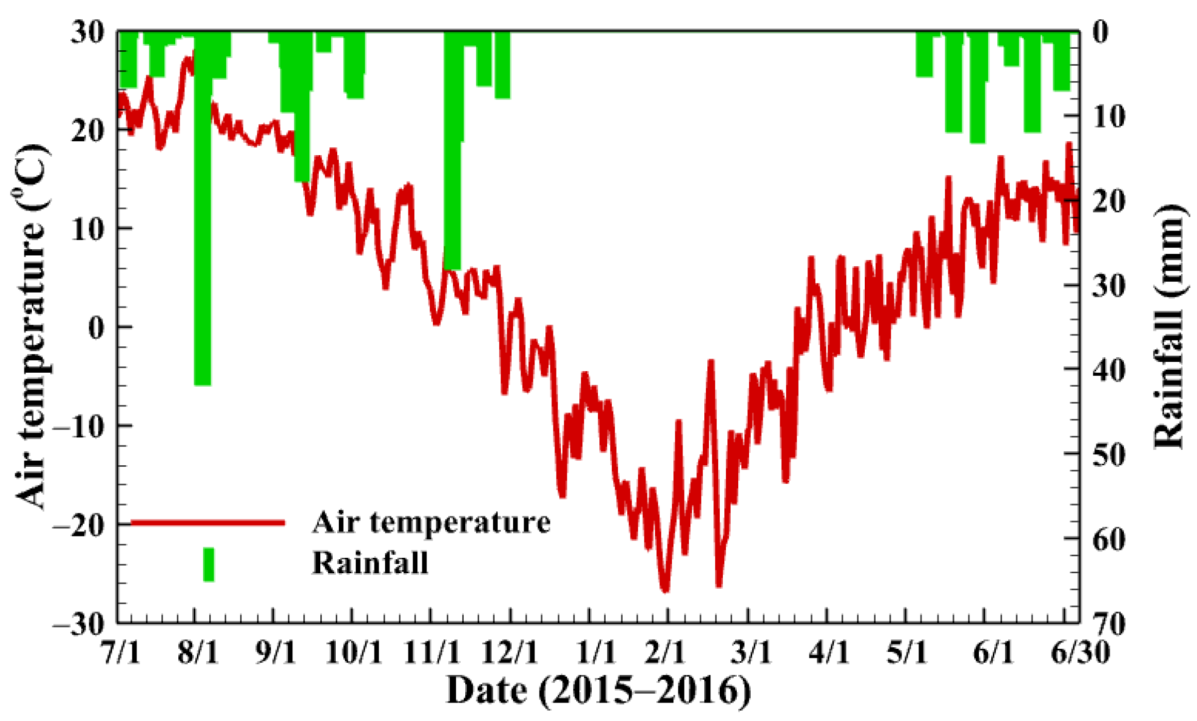
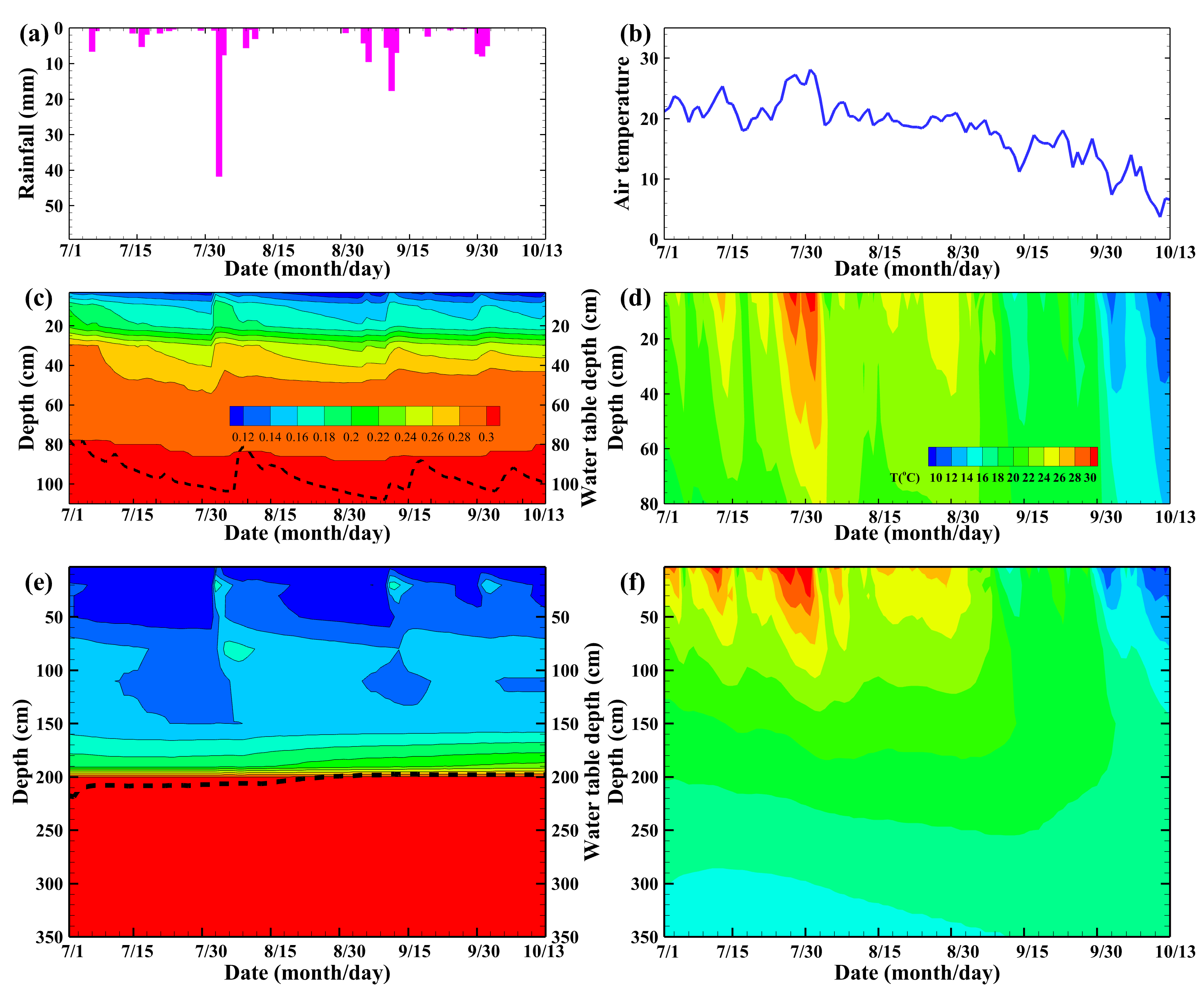
4.1. Observed Results

The field experiments show that the moisture content was very responsive to the precipitation in both lysimeters (left panel in Figure 4). This response became stronger with larger precipitation (compare the moisture content response between August 1 and September 10 in both Figure 4c and Figure 4e). In addition, the magnitude of the moisture content response was generally stronger close to the land surface due to direct effects of precipitation and solar radiation. This magnitude of response became weaker with depth, with some exceptions probably caused by local-scale soil heterogeneity. For example, in lysimeter 1, the mean moisture content at 3, 20, 30, and 80 cm in lysimeter 1 was 0.077, 0.15, 0.13, and 0.31, but the standard deviation gradually decreased (i.e., 0.020, 0.016, 0.013, and 0.0014, respectively).

Groundwater levels in both lysimeters varied differently (Figure 4c,e). In lysimeter 1 (Figure 4c), the groundwater level gradually declined when there was negligible rain (<5 mm/d) but rose rapidly when rain was sufficiently heavy. This indicates that the shallow groundwater contributed to the evaporation. The water table fluctuation also indicates that the groundwater evaporation extinction depth is approximately 105 cm below the land surface (Figure 4c). In comparison, the groundwater level in lysimeter 2 (Figure 4e) rose steadily with a total of 13.8 cm increase by the end of the experiment. The groundwater level was always deeper than 105 cm and so the groundwater in lysimeter 2 was gaining recharge throughout the experimental period. If the monitoring was continued, we would observe that the groundwater level would continue to increase until it reached the groundwater evaporation extinction depth.

The variation in the soil temperature in both lysimeters did not differ significantly (Figure 4d,f). Overall, the soil temperature decreased with depth from July to late September when the air temperature was higher than the groundwater temperature (approximately 15 °C as shown in Figure 4f), whereas it increased with depth after late September when the air temperature was lower than the groundwater temperature. The extent of the vertical temperature changes across the lysimeter profiles was generally dependent on the weather condition (air temperature, the duration of sunny days, precipitation, etc.). For example, the soil temperature continued to increase with time and depth between 23 July and 30 July, but the increased soil temperature particularly at the land surface was quickly reduced to the air temperature once precipitation occurred on 3 August.

4.2. Model Calibration and Validation

The soil moisture and soil temperature of both lysimeters were simulated simultaneously for the period from 1 July to 13 October 2015 (Figure 5). The first one-third of all the time series was used for model calibration, whereas the rest was for model validation. The optimized $K_s$ shown in Table 1 and Table 2 is less than the mean $K_s$ obtained from the double-ring infiltrometer experiment. This difference indicates the limitation of the infiltration test [38].

The simulated soil moisture fitted the observation reasonably well at all depths. The models were able to reproduce the rapid increases in the soil moisture after precipitation infiltration but were unable to capture the peaks. This may be due to the reduction in the unsaturated hydraulic conductivity of the dry soil surface layer between the atmosphere and the wet soil layer below [39,40]. Overall, the maximum $RE$ and $RMSE$ of the soil moisture are 6.1% and 0.012 cm³/cm³ in lysimeter 1 and 6.47% and 0.016 cm³/cm³ in lysimeter 2, respectively.

The results include soil moisture and temperature. The simulated soil temperature also achieved reasonable fitting to the observation (Figure 5). Fitting to soil surface temperature is generally difficult because of strong variability caused by complex soil–atmosphere interactions [41]. Our models were only able to fit the trends of the surface-soil temperature rather than the exact variability. In comparison, fitting to the soil moisture at deeper locations was relatively easier because of less variability. Overall, the maximum $RE$ and $RMSE$ of the soil temperature are 4.12% and 2.57 °C in lysimeter 1 and 8.91% and 3.42 °C in lysimeter 2, respectively.

4.3. Cumulative Evaporation

The cumulative measured evaporation over the study period was 24.06 and 13.48 cm for lysimeters 1 and 2, respectively (red and blue open circles in Figure 6). In comparison, the isothermal models (liquid water flow only) produced the cumulative evaporation of 20.52 and 7.52 cm for lysimeters 1 and 2 (red and blue solid curves), respectively, whereas the nonisothermal models (both liquid and vapor water flow) yielded the cumulative evaporation of 24.29 and 12.78 cm for lysimeters 1 and 2 (red and blue dashed curves), respectively. As a result, the isothermal models underestimated the cumulative evaporation by 14.7% in lysimeter 1 and 44.2% in lysimeter 2, respectively. The nonisothermal models produced more accurate cumulative evaporation with 0.95% overestimation in lysimeter 1 and 5.2% underestimation in lysimeter 2, respectively. The more accurate results from the nonisothermal models are due to the consideration of the effects of soil temperature and vapor flux on evaporation.

The model simulations show significantly different contributions of liquid water and water vapor to evaporation in lysimeters 1 and 2. As demonstrated on the left panel of Figure 7, the total flux in lysimeter 1 was always directed upwards and the water transfer was mainly due to liquid water flow driven by pressure head and temperature gradients. The vapor flux was relatively small compared with liquid water flux. Therefore, it need not consider vapor flux in lysimeter 1. However, the direction of the total flux in lysimeter 2 changes even at diurnal scales (right panel of Figure 7). Both the liquid water and water vapor fluxes are directed upwards from approximately 22:00 to 11:00. This result indicates that the evaporation mainly occurs during night time in lysimeter 2. The water vapor flux becomes dominant, and the net water flow is directed downwards from around 12:00 to 22:00. The downward water vapor flux implies a condensation process within the soil profile, resulting in the increase in the soil moisture.

4.4. Liquid Water and Water Vapor Fluxes

Evaporation rates are composed of both liquid water and water vapor fluxes. In lysimeter 1, liquid water fluxes had more significant contribution to evaporation than water vapor fluxes as the magnitude of liquid water fluxes was greater (compare Figure 8a and Figure 8b).

In general, water vapor fluxes were episodic and only occurred when rain was absent and the air temperature was appropriate. As shown in Figure 8a,c, water vapor fluxes mainly occurred between the soil surface and 20 cm below in both lysimeters. The depth generally decreased from July to October due to the decrease in air temperature. For example, the average depth of water vapor fluxes in lysimeter 2 was approximately 20, 15, and 10 cm for July, August, and September, respectively (Figure 8c). Interestingly, water vapor fluxes in lysimeter 1 (Figure 8a) were relatively small compared to those in lysimeter 2 (Figure 8c). In addition, the soil temperature near the surface ground in lysimeter 2 was higher than that in lysimeter 1. For example, the daily variations of soil temperature on 30 July were 21.2 (from 20.4 to 41.6 °C) and 28.4 °C (from 21.1 to 49.6 °C) in lysimeter 1 and 2, respectively. The higher soil temperature near the surface ground resulted in larger thermal gradient in lysimeter 2 than that in lysimeter 1 (Figure 9). As a consequence, the water vapor fluxes were larger in lysimeter 2 than those in lysimeter 1.

.

Liquid water flux distributions are different between the two lysimeters. The liquid water in lysimeter 1 was always transported upward except for rainy days (Figure 8b), whilst it could flow both upward and downward at the same time in lysimeter 2. This difference was attributed to the difference in the water table depth.

Liquid water flux distributions in two lysimeters could differ significantly at hourly scales. As shown in Figure 8b1, the liquid water fluxes in lysimeter 1 were relatively small near the surface ground from 0:00 to 10:00 (0.0001~0.032 cm/h) and then became quite large from approximately 10:00 to 17:00 (0.032~0.094 cm/h). In comparison, the liquid water fluxes in lysimeter 2 were negative near the surface groundwater from 0:00 to 8:00 (−0.001~−0.0037 cm/h). The fluxes were maintained at approximately 0.002 cm/h between 8:00 and 22:00 before dropping dramatically to nearly 0 afterwards. Another difference in the liquid water fluxes between the two lysimeters is that the liquid water fluxes between 2 and 10 cm were relatively large and always positive (upwards flow) in lysimeter 2. This may be due to upward flowing water from the lower layer that accumulates below the surface layer where the unsaturated hydraulic conductivity is small.

Based on some studies [42,43], the evaporation front occurred where the liquid and vapor fluxes are equal. Note that the vapor flux mainly occurred above 5 cm in lysimeter 1. However, liquid water flux dominates near the surface ground. Therefore, the evaporation front is located at the surface ground in lysimeter 1. However, water vapor flux occurred above around 30 cm in lysimeter 2, and it dominates above around 15–25 cm at different times. Therefore, the evaporation front is located at the depth of around 15–25 cm for lysimeter 2 (Figure 10). Additionally, we calculated the hydraulic head in both lysimeters. It can be found that there is no zero-flux plane in lysimeter 1 except for rainy days. This means that net water transport is directed upwards and constantly consumes groundwater. However, there exists a zero-flux plane located at around 0–50 cm in lysimeter 2 except for rainy days (Figure 10). This indicated that the maximum depth of evaporation front was not exceeding the location of zero-flux plane.

5. Discussion

5.1. Effect of Isothermal and Nonisothermal Models on the Evaporation

The analysis reveals that the evaporation front in lysimeter 1 is located at the surface ground, indicating that evaporation is in the atmosphere-limited stage. This explains why cumulative evaporation in lysimeter 1 is nearly twice that in lysimeter 2 during the experimental period. To further investigate the mechanisms underlying the isothermal and nonisothermal models, three additional numerical models were set up: an isothermal model in lysimeter 1, an isothermal model in lysimeter 2, and a nonisothermal model in lysimeter 2 that neglects vapor flux. The maximum $RE$ and $RMSE$ of the soil moisture are 3.0% and 0.01 cm³/cm³ in isothermal model 1, 4.87% and 0.016 cm³/cm³ in isothermal model 2, and 4.8% and 0.01 cm³/cm³ in nonisothermal model 2, respectively. These errors are consistent with those of previous models, and the simulated soil moisture and temperature align well with observed data (Figure 5), indicating those models’ reliability for evaporation calculations.

The cumulative evaporation of isothermal model 1, isothermal model 2, and nonisothermal model 2 was 47.71, 7.93, and 9.88 cm (Figure 11), respectively. However, isothermal model 1 overestimated evaporation by 98.3%, while isothermal model 2 and nonisothermal model 2 underestimated it by 41.2% and 26.7%, respectively. This implied that while the models accurately simulate soil moisture and temperature, they exhibit significant errors in estimating cumulative evaporation. Wang et al. [21] conducted lab experiments to investigate the effect of isothermal and nonisothermal models on evaporation under the conditions of different water table depths. They found that the nonisothermal model, which couples water and heat transport, closely matches observed values, with a maximum evaporation error of only 2.34% when the water table depth is below the evaporation limit. In contrast, the isothermal model produced larger errors, exceeding 77.35%, primarily due to the overestimation of evaporation rates by the Penman–Montheith (P–M) model [44]. This overestimation has been corroborated by other studies [45,46,47].

The impact of soil temperature on liquid water flux cannot be overlooked, even when soil moisture near the surface is relatively high. Thermal gradients between upper and lower soil layers drive water flux from warmer to cooler regions, influenced by temperature-induced increases in the pressure of both vapor and liquid phases. Despite the significant role of soil temperature in evaporation and infiltration processes, it is often neglected in practical water resource assessments [48].

In lysimeter 2, evaporation is in the soil-limited stage, requiring consideration of both the nonisothermal model and water vapor flux. At this time, liquid water flux and water vapor flux coexist, with vapor flux dominating above the evaporation front (Figure 7b). The isothermal models underestimated cumulative evaporation by 44.2% and 41.2% (Figure 6 and Figure 11), while the nonisothermal model underestimated it by 26.7% (Figure 11). This highlights distinct evaporation mechanisms compared to lysimeter 1. In lysimeter 2, vapor flux contributes significantly to the total flux, driven by temperature gradients. The limited liquid water storages in the upper soil layers increases air-filled porosity, facilitating vapor flux. Several studies have emphasized the importance of spatial temperature gradients in driving vapor fluxes, which play an important role in soil mass and energy transfer [39,49]. Bittelli et al. [39] further demonstrated that vapor flow can induce sinusoidal variations in near-surface-soil moisture using a couple numerical model. However, other researchers have argued that spatial temperature gradients do not always produce obviously vapor fluxes [23,33].

Our findings suggest that the influence of spatial temperature gradients on vapor fluxes depends on the water table depth under consistent atmospheric conditions. During the atmosphere-limited stage, the nonisothermal model provides more accurate evaporation predictions. In contrast, during the soil-limited stage, vapor flux must be explicitly considered. Additionally, diurnal variations in lysimeter 2, particularly during condensation phases, are driven by nighttime cooling, which enhances vapor flux toward the surface and promotes condensation. This is critical for understanding the dynamic interplay between liquid and vapor fluxes in the soil profile.

5.2. Limitations

Firstly, although we know that the lysimeters were homogeneously packed with the same local soil before the experiments, running HYDRUS-1D using the initial hydraulic parameters and single layers did not allow for reasonable fitting to soil moisture and temperature time series simultaneously. Using spatially uniform soil’s hydraulic properties in the numerical models does not obtain a satisfied simulation of the measured soil moisture and temperature for both groundwater levels. Many studies [38,42,50] have encountered similar problems. According to Jiménez-Martínez [50], the model results agree fairly well with the observation data by considering the spatial variability of soil properties, which may be modified as a result of salt movement during evaporation [36].

Secondly, the entire experimental period (about 3 months), which used one month to calibrate and two months to validate model, was relatively short. The strongest evaporation occurred in July and August in the study area. To investigate the evaporation mechanism under the different water table depths, the entire experimental period (from July to October) can meet the requirements of this study. However, extending the study period could provide deeper insights into seasonal evaporation trends, particularly during periods of lower evaporation rates or under varying climatic conditions. This would enhance our understanding of the long-term dynamics of evaporation and its implications for water management in semi-arid regions. Additionally, the scalability of our findings to other semi-arid regions or conditions beyond the study area remains to be explored.

Thirdly, while the nonisothermal model demonstrates improved accuracy in evaporation predictions, its limitations in specific scenarios, for example, extreme temperature gradients, should be critically evaluated. For instance, under extreme temperature gradients, the model may overestimate vapor flux due to simplified assumptions about heat and water transport.

Lastly, while the impact of vapor flux on evaporation in lysimeter 2 is convincingly argued, stronger connections to broader implications for water management practices in semi-arid regions are needed. For example, understanding the role of vapor flux in soil water dynamics can inform irrigation scheduling, soil moisture conservation strategies, and the design of water-efficient agricultural systems. By integrating these insights into practical water management frameworks, our findings can contribute to more sustainable water use in water-scarce environments.

6. Conclusions

This study investigated the impact of water table depths on evaporation processes in semi-arid regions with shallow groundwater through field experiments and numerical modeling using the HYDRUS-1D model. Two lysimeters with different water table depths (1.2 m and 4.2 m) were set up in the Ordos Basin, Northwest China, and instrumented with multi-depth soil moisture and temperature sensors.

(1)

The cumulative evaporation measured over the experimental period was 24.06 cm and 13.48 cm for lysimeter 1 and 2. The isothermal models underestimated cumulative evaporation by 14.7% and 44.2% for lysimeter 1 and 2. In contrast, the nonisothermal models produced more accurate results, with only 0.95% and overestimation and 5.2% underestimation, respectively.

(2)

In lysimeter 1, liquid water flux dominated the evaporation process, driven by pressure head and temperature gradients. In lysimeter 2, water vapor flux played a significant role, especially during nighttime, with condensation processes occurring within the soil profile during the day.

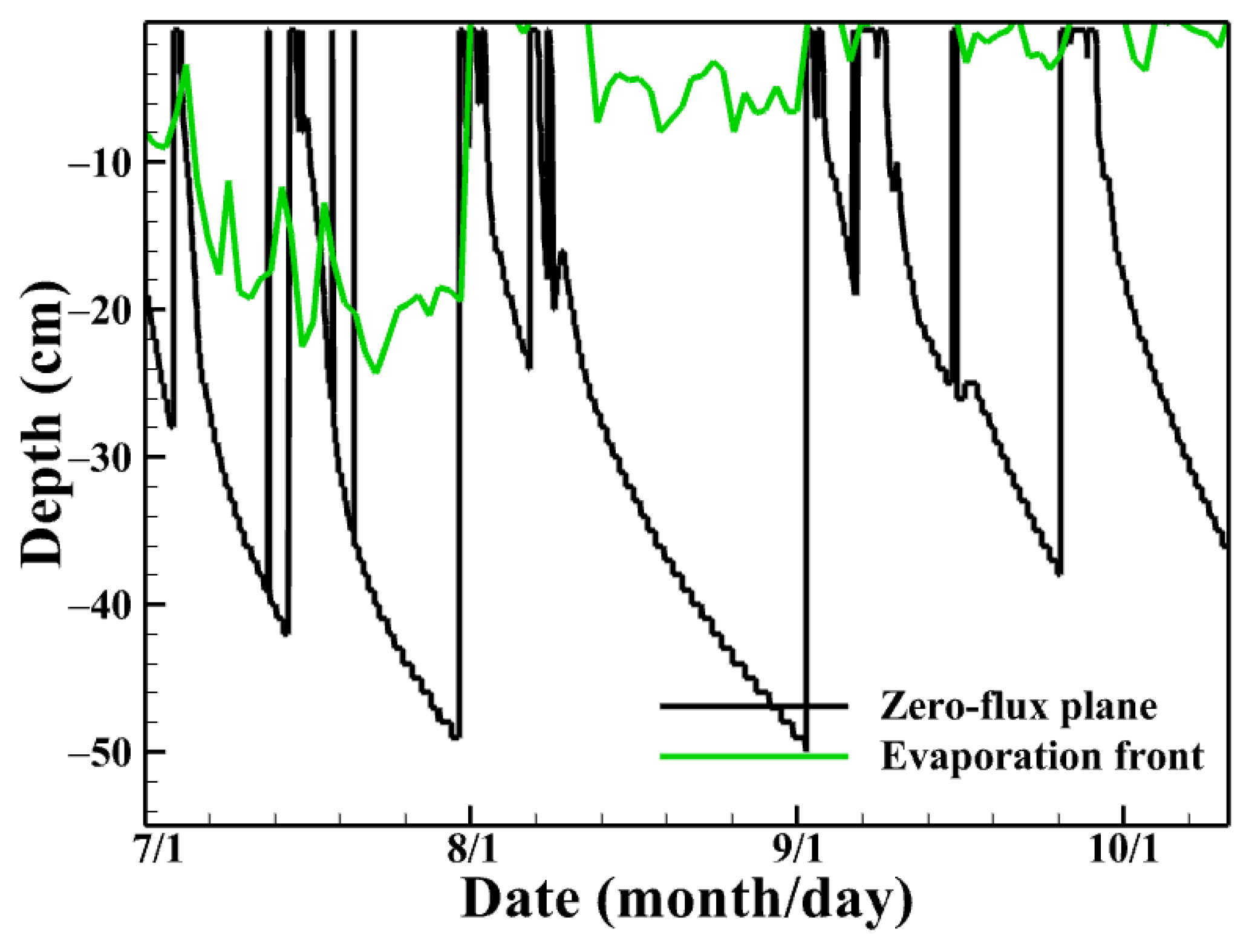
(3)

The evaporation front was located at the surface in lysimeter 1, while it was found at a depth of 15–25 cm in lysimeter 2. The zero-flux plane was absent in lysimeter 1 but present at 0–50 cm in lysimeter 2.

(4)

The nonisothermal models, which accounted for both liquid and vapor water fluxes, provided more accurate evaporation estimates compared to the isothermal models. This highlights the importance of considering soil temperature and vapor flux in evaporation models, particularly in arid and semi-arid regions.

The research hypothesis that the depth of the shallow water table significantly influences soil evaporation rates under natural conditions, and that non-isothermal processes play a critical role in arid and semi-arid regions, was confirmed. The findings underscore the necessity of incorporating both water and heat transport in numerical models to enhance the accuracy of evaporation estimates. However, the study has some limitations, including the relatively short experimental period (three months). Future research should extend the experimental duration. Additionally, further studies could explore the impact of vegetation and different soil types on evaporation processes in the presence of shallow groundwater.

References

1. Good, S.P.; Noone, D.; Bowen, G. Hydrologic connectivity constrains partitioning of global terrestrial water fluxes. Science 2015, 349, 175–177. [Google Scholar] [PubMed]
2. Seneviratne, S.I.; Corti, T.; Davin, E.L.; Hirschi, M.; Jaeger, E.B.; Lehner, I.; Orlowsky, B.; Teuling, A.J. Investigating soil moisture–climate interactions in a changing climate: A review. Earth-Sci. Rev. 2010, 99, 125–161. [Google Scholar] [CrossRef]
3. Kahil, M.T.; Dinar, A.; Albiac, J. Modeling water scarcity and droughts for policy adaptation to climate change in arid and semiarid regions. J. Hydrol. 2015, 522, 95–109. [Google Scholar] [CrossRef]
4. Shoba, P.; Ramakrishnan, S.S. Modeling the contributing factors of desertification and evaluating their relationships to the soil degradation process through geomatic techniques. Solid Earth 2016, 7, 341–354. [Google Scholar]
5. Allan, R.P.; Barlow, M.; Byrne, M.P.; Cherchi, A.; Douville, H.; Fowler, H.J.; Gan, T.Y.; Pendergrass, A.G.; Rosenfeld, D.; Swann, A.L. Advances in understanding large-scale responses of the water cycle to climate change. Ann. N. Y. Acad. Sci. 2020, 1472, 49–75. [Google Scholar] [PubMed]
6. Gong, C.; Wang, W.; Zhang, Z.; Wang, H.; Luo, J.; Brunner, P. Comparison of field methods for estimating evaporation from bare soil using lysimeters in a semi-arid area. J. Hydrol. 2020, 590, 125334. [Google Scholar]
7. Sakai, M.; Jones, S.B.; Tuller, M. Numerical evaluation of subsurface soil water evaporation derived from sensible heat balance. Water Resour. Res. 2011, 47, W02547. [Google Scholar]
8. Smits, K.M.; Ngo, V.V.; Cihan, A.; Sakaki, T.; Illangasekare, T.H. An evaluation of models of bare soil evaporation formulated with different land surface boundary conditions and assumptions. Water Resour. Res. 2012, 48, W12522. [Google Scholar] [CrossRef]
9. Veihmeyer, F.J.; Brooks, F.A. Measurements of cumulative evaporation from bare soil. Eos Trans. Am. Geophys. Union 1954, 35, 601–607. [Google Scholar]
10. Gardner, W.R.; Fireman, M. Laboratory studies of evaporation from soil columns in the presence of a water table. Soil Sci. 1958, 85, 244–249. [Google Scholar] [CrossRef]
11. Shih, S.F. Soil surface evaporation and water table depths. J. Irrig. Drain. Eng. ASCE 1983, 109, 366–376. [Google Scholar]
12. Hellwig, D.H.R. Evaporation of water from sand, 4: The influence of the depth of the water-table and the particle size distribution of the sand. J. Hydrol. 1973, 18, 317–327. [Google Scholar] [CrossRef]
13. Coudrain-Ribstein, A.; Pratx, B.; Talbi, A.; Jusserand, C. Is the evaporation from phreatic aquifers in arid zones independent of the soil characteristics? C. R. L’acad. Sci.—Ser. IIA—Earth Planet. Sci. 1998, 326, 159–165. [Google Scholar]
14. Warrick, A.W.; Yitayew, M. Trickle lateral hydraulics. I: Analytical solution. J. Irrig. Drain. Eng. ASCE 1988, 114, 281–288. [Google Scholar] [CrossRef]
15. Shokri, N.; Salvucci, G.D. Evaporation from porous media in the presence of a water table. Vadose Zone J. 2011, 10, 1309–1318. [Google Scholar] [CrossRef]
16. Yang, G.; Xu, R.; Tian, Y.; Guo, S.; Wu, J.; Chu, X. Data-driven methods for flow and transport in porous media: A review. Int. J. Heat Mass Transf. 2024, 235, 126149. [Google Scholar]
17. Yonaba, R.; Kiema, A.; Tazen, F.; Belemtougri, A.; Cissé, M.; Mounirou, L.A.; Bodian, A.; Koïta, M.; Karambiri, H. Accuracy and interpretability of machine learning-based approaches for daily ETo estimation under semi-arid climate in the West African Sahel. Earth Sci. Inform. 2025, 18, 87. [Google Scholar] [CrossRef]
18. Eshetu, K.D.; Alamirew, T.; Woldesenbet, T.A. Interpretable machine learning for predicting evaporation from awash reservoirs, Ethiopia. Earth Sci. Inform. 2023, 16, 3209–3226. [Google Scholar] [CrossRef]
19. Rose, D.; Konukcu, F.; Gowing, J. Effect of watertable depth on evaporation and salt accumulation from saline groundwater. Aust. J. Soil Res. 2005, 43, 565–573. [Google Scholar]
20. Gowing, J.W.; Konukcu, F.; Rose, D.A. Evaporative flux from a shallow watertable: The influence of a vapour–liquid phase transition. J. Hydrol. 2006, 321, 77–89. [Google Scholar]
21. Wang, W.; Zhao, G.; Li, J.; Hou, L.; Li, Y.; Yang, F. Experimental and numerical study of coupled flow and heat transport. Proc. Inst. Civ. Eng.—Water Manag. 2011, 164, 533–547. [Google Scholar]
22. Wang, W.; Zhang, Z.; Yeh, T.-c.J.; Qiao, G.; Wang, W.; Duan, L.; Huang, S.-Y.; Wen, J.-C. Flow dynamics in vadose zones with and without vegetation in an arid region. Adv. Water Resour. 2017, 106, 68–79. [Google Scholar]
23. Goss, K.-U.; Madliger, M. Estimation of water transport based on in situ measurements of relative humidity and temperature in a dry Tanzanian soil. Water Resour. Res. 2007, 43, W05433. [Google Scholar]
24. D’Odorico, P.; Bhattachan, A.; Davis, K.F.; Ravi, S.; Runyan, C.W. Global desertification: Drivers and feedbacks. Adv. Water Resour. 2013, 51, 326–344. [Google Scholar]
25. Dong, X.; Zhang, X. Some observations of the adaptations of sandy shrubs to the arid environment in the Mu US Sandland: Leaf water relations and anatomic features. J. Arid. Environ. 2001, 48, 41–48. [Google Scholar]
26. Huang, J.; Zhou, Y.; Hou, R.; Wenninger, J. Simulation of water use dynamics by Salix bush in a semiarid shallow groundwater area of the Chinese Erdos Plateau. Water 2015, 7, 6999–7021. [Google Scholar] [CrossRef]
27. Yin, L.; Zhou, Y.; Huang, J.; Wenninger, J.; Zhang, E.; Hou, G.; Dong, J. Interaction between groundwater and trees in an arid site: Potential impacts of climate variation and groundwater abstraction on trees. J. Hydrol. 2015, 528, 435–448. [Google Scholar]
28. Gao, N.; Liang, W.; Gou, F.; Liu, Y.; Fu, B.; Lü, Y. Assessing the impact of agriculture, coal mining, and ecological restoration on water sustainability in the Mu US Sandyland. Sci. Total Environ. 2024, 929, 172513. [Google Scholar]
29. Zhang, Z.; Wang, W.; Wang, Z.; Chen, L.; Gong, C. Evaporation from bare ground with different water-table depths based on an in-situ experiment in Ordos Plateau, China. Hydrogeol. J. 2018, 26, 1683–1691. [Google Scholar]
30. Van Genuchten, M. A closed-form equation for predicting the hydraulic conductivity of unsaturated soils. Soil Sci. Soc. Am. J. 1980, 44, 892–898. [Google Scholar]
31. Lai, J.; Ren, L. Assessing the size dependency of measured hydraulic conductivity using double-ring infiltrometers and numerical simulation. Soil Sci. Soc. Am. J. 2007, 71, 1667–1675. [Google Scholar] [CrossRef]
32. Simunek, J.J.; Šejna, M.; Saito, H.; Sakai, M.; Van Genuchten, M. The HYDRUS-1D Software Package for Simulating the Movement of Water, Heat, and Multiple Solutes in Variably Saturated Media; Version 4.17; University of California Riverside: Riverside, CA, USA, 2013. [Google Scholar]
33. Saito, H.; Šimůnek, J.; Mohanty, B.P. Numerical analysis of coupled water, vapor, and heat transport in the vadose zone. Vadose Zone J. 2006, 5, 784–800. [Google Scholar] [CrossRef]
34. Marsily, G.D. Quantitative Hydrogeology: Groundwater Hydrology for Engineers; Academic Press: Cambridge, MA, USA, 1986. [Google Scholar]
35. Chung, S.O.; Horton, R. Soil heat and water flow with a partial surface mulch. Water Resour. Res. 1987, 23, 2175–2186. [Google Scholar] [CrossRef]
36. Cortés, V.B.F. Sar Effects on Evaporation Fluxes from Shallow Groundwater. Master’s Thesis, Pontificia Universidad Catolica de Chile, Santiago, Chile, 2015. [Google Scholar]
37. Camillo, P.J.; Gurney, R.J. A resistance parameter for bare-soil evaporation models. Soil Sci. 1986, 141, 95–105. [Google Scholar] [CrossRef]
38. Hou, L.; Wang, X.-S.; Hu, B.X.; Shang, J.; Wan, L. Experimental and numerical investigations of soil water balance at the hinterland of the Badain Jaran desert for groundwater recharge estimation. J. Hydrol. 2016, 540, 386–396. [Google Scholar] [CrossRef]
39. Bittelli, M.; Ventura, F.; Campbell, G.S.; Snyder, R.L.; Gallegati, F.; Pisa, P.R. Coupling of heat, water vapor, and liquid water fluxes to compute evaporation in bare soils. J. Hydrol. 2008, 362, 191–205. [Google Scholar] [CrossRef]
40. Han, J.; Zhou, Z.; Fu, Z.; Wang, J. Evaluating the impact of nonisothermal flow on vadose zone processes in presence of a water table. Soil Sci. 2014, 179, 57–67. [Google Scholar] [CrossRef]
41. Saito, H.; Šimůnek, J. Effects of meteorological models on the solution of the surface energy balance and soil temperature variations in bare soils. J. Hydrol. 2009, 373, 545–561. [Google Scholar] [CrossRef]
42. Hernández-López, M.F.; Braud, I.; Gironás, J.; Suárez, F.; Muñoz, J.F. Modelling evaporation processes in soils from the Huasco salt flat basin, Chile. Hydrol. Process. 2016, 30, 4704–4719. [Google Scholar] [CrossRef]
43. Hernández-López, M.F.; Gironás, J.; Braud, I.; Suárez, F.; Muñoz, J.F. Assessment of evaporation and water fluxes in a column of dry saline soil subject to different water table levels. Hydrol. Process. 2014, 28, 3655–3669. [Google Scholar] [CrossRef]
44. Zhang, Z.; Wang, W.; Gong, C.; Zhao, M.; Wang, Z.; Ma, H. Effects of non-isothermal flow on groundwater recharge in a semi-arid region. Hydrogeol. J. 2021, 29, 541–549. [Google Scholar] [CrossRef]
45. Liu, T.; Liu, L.; Luo, Y.; Lai, J. Simulation of groundwater evaporation and groundwater depth using swat in the irrigation district with shallow water table. Environ. Earth Sci. 2015, 74, 315–324. [Google Scholar] [CrossRef]
46. Ortega-Farias, S.O.; Olioso, A.; Fuentes, S.; Valdes, H. Latent heat flux over a furrow-irrigated tomato crop using penman–monteith equation with a variable surface canopy resistance. Agric. Water Manag. 2006, 82, 421–432. [Google Scholar] [CrossRef]
47. Zhang, B.; Kang, S.; Li, F.; Zhang, L. Comparison of three evapotranspiration models to Bowen ratio-energy balance method for a vineyard in an arid desert region of northwest China. Agric. For. Meteorol. 2008, 148, 1629–1640. [Google Scholar] [CrossRef]
48. Cheng, Y.; Zhan, H.; Yang, W.; Dang, H.; Li, W. Is annual recharge coefficient a valid concept in arid and semi-arid regions? Hydrol. Earth Syst. Sci. 2017, 21, 5031–5042. [Google Scholar] [CrossRef]
49. Scanlon, B.R.; Milly, P.C.D. Water and heat fluxes in desert soils: 2. Numerical simulations. Water Resour. Res. 1994, 30, 721–733. [Google Scholar] [CrossRef]
50. Jiménez-Martínez, J.; Skaggs, T.H.; van Genuchten, M.T.; Candela, L. A root zone modelling approach to estimating groundwater recharge from irrigated areas. J. Hydrol. 2009, 367, 138–149. [Google Scholar] [CrossRef]
Figure 1. Study area location map. (a) Location of the Mu Us Sandy Land in China; (b) Location of the experimental site in the Mu Us Sandy Land; (c) Photo of one lysimeter outcrop. The boundary of the Mu Us Sandy Land is from Gao, et al. [28].
Water 17 01113 g001
Figure 2. Rainfall and air temperature at the field site from 1 July 2015 to 30 June 2016. (Revised from Zhang, et al. [29]).
Water 17 01113 g002
Figure 3. Diagram of lysimeters and corresponding monitoring schemes. Sensors (soil moisture and temperature) were installed at (a) 3–80 cm and (b) 10–350 cm below ground to record soil moisture, and divers were placed near the bottom to measure groundwater depth.
Water 17 01113 g003
Figure 4. Observed values of soil moisture, temperature, and water table depths during the experimental period. (a,b) represent rainfall and air temperature, respectively; (c,e) represent soil moisture in lysimeters 1 and 2, respectively. Black dotted lines in (c,e) indicate water table depths; (d,f) represent soil temperature in lysimeters 1 and 2, respectively.
Water 17 01113 g004
Figure 5. Comparison between observed and simulated results for the depths of (a) 3, (b) 20, and (c) 80 cm of soil moisture and (d) 3, (e) 20 and (f) 80 of soil temperature in lysimeter 1 and (g) 10, (h) 80, and (i) 190 cm of soil moisture and (j) 10, (k) 80, and (l) 190 cm of soil temperature in lysimeter 2, respectively.
Water 17 01113 g005
Figure 6. Variation in cumulative evaporation in both lysimeters. Red and blue colors represent cumulative evaporation in lysimeters 1 and 2, respectively.
Water 17 01113 g006
Figure 7. Liquid and water vapor fluxes near the surface ground for different water table depths at different time, 0:00 (a,b), 6:00 (c,d), 12:00 (e,f) and 18:00 (g,h) in lysimeter 1 and 2 on 30 July 2015. Left and right panels show liquid and water vapor fluxes in lysimeter 1 and 2, respectively. Up and down arrows correspond to downward and upward water movement, respectively.
Water 17 01113 g007
Figure 8. Variation in water vapor flux in lysimeter 1 (a), liquid water flux in lysimeter 1 (b), water vapor flux in lysimeter 2 (c), and liquid water flux in lysimeter 2 (d) from 1 July to 13 October 2015. (b1,d1) show variation of liquid water flux on 30 July in both lysimeters, respectively. Positive and negative values represent upward and downward fluxes, respectively.
Water 17 01113 g008
Figure 9. The variation of soil temperature gradient on 30 July in (a) lysimeter 1 and (b) lysimeter 2, respectively. Soil temperature gradient was computed using T 2 T 1 z .
Water 17 01113 g009
Figure 10. The distributions of zero-flux plane and evaporation front in lysimeter 2.
Water 17 01113 g010
Figure 11. Variation in cumulative evaporation in both lysimeters. Red and blue color represent cumulative evaporation in lysimeters 1 and 2, respectively (Isothermal 1 and 2 represented isothermal model in lysimeter 1 and 2, respectively. Nonisothermal 2 represented nonisothermal model, which ignored the vapor flux in lysimeter 2).
Water 17 01113 g011