Bivariate and Partial Wavelet Coherence for Revealing the Remote Impacts of Large-Scale Ocean-Atmosphere Oscillations on Drought Variations in Xinjiang, China


Abstract
1. Introduction
2. Materials and Methods
2.1. Study Area
2.2. Data
2.3. Methods
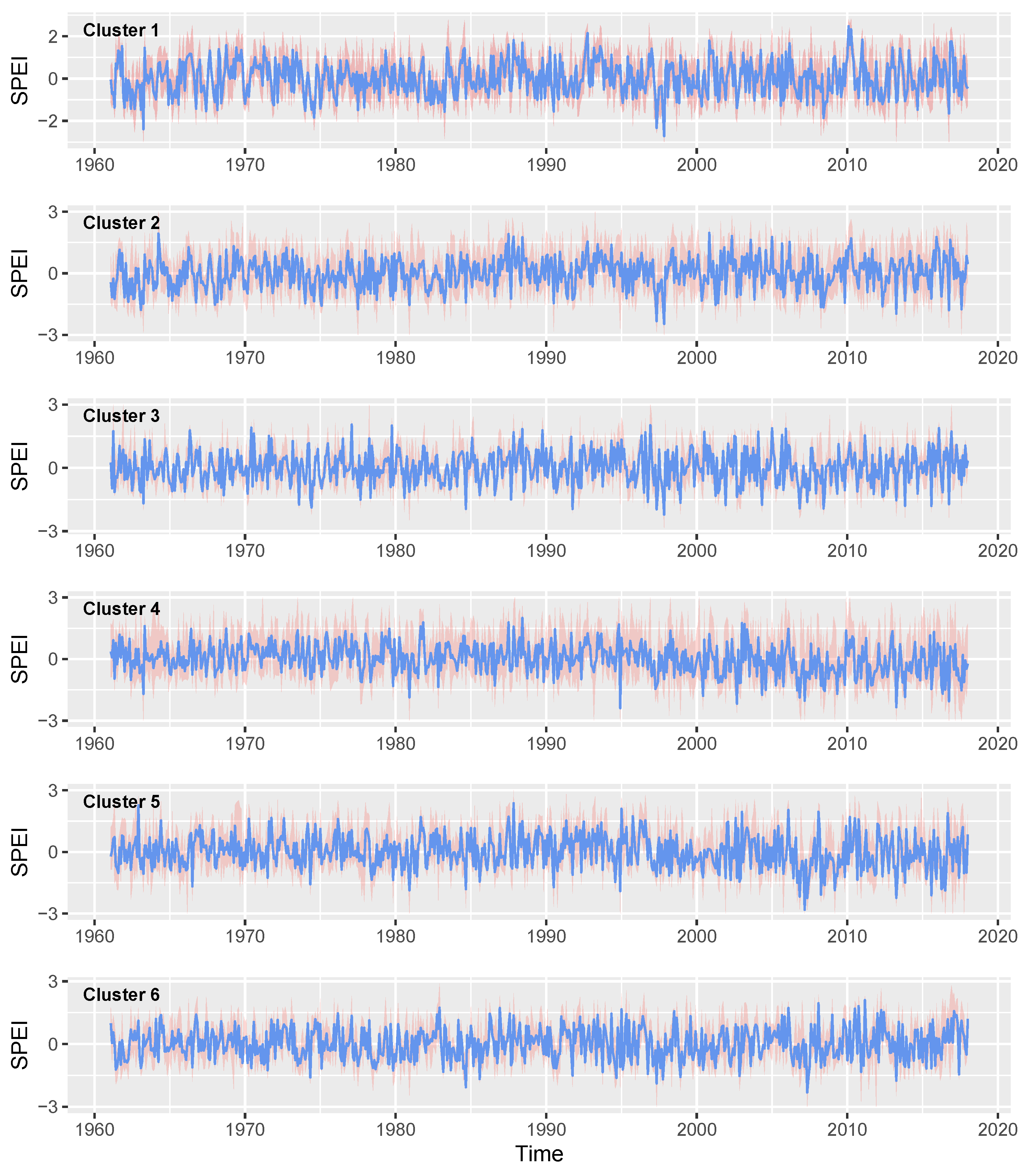
2.3.1. SPEI
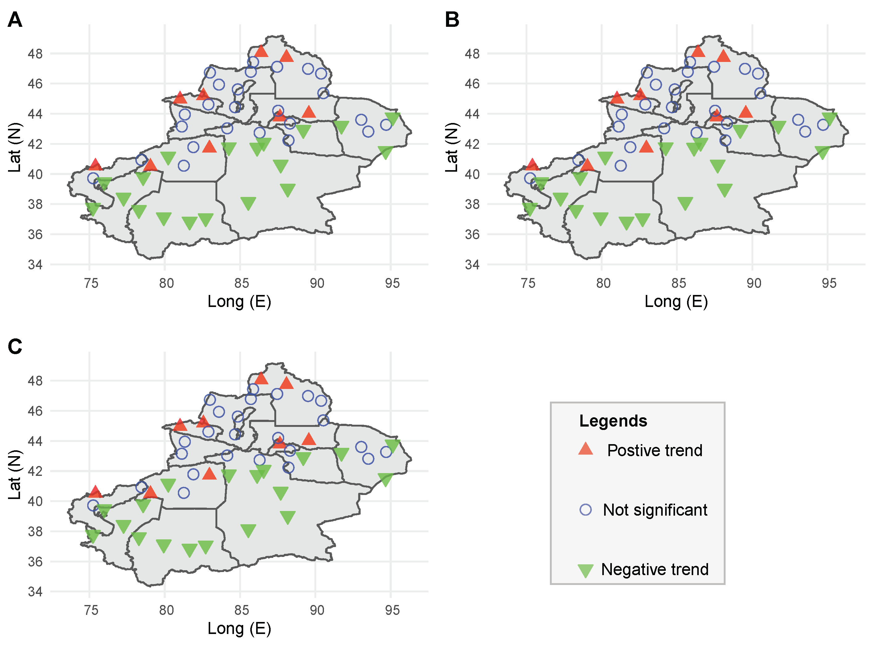
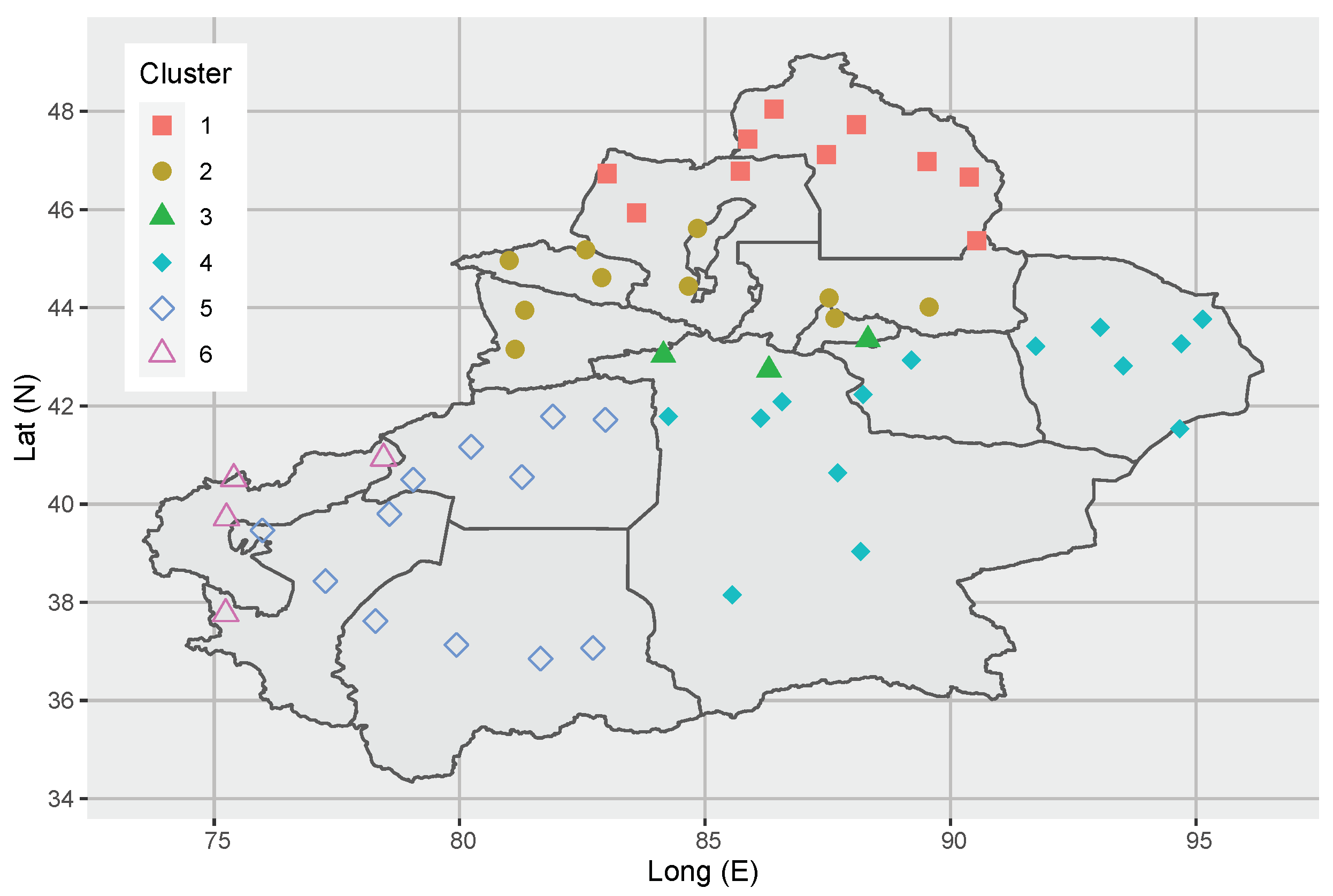
2.3.2. Seasonal Kendall Test and Hierarchical Clustering
2.3.3. Correlation Analysis and Partial Correlation Analysis
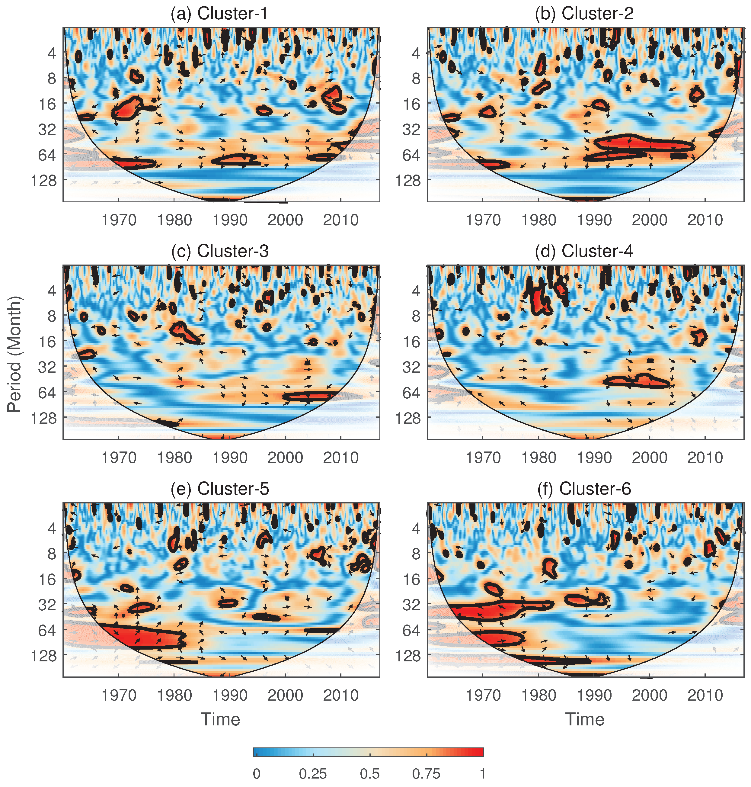
2.3.4. A Brief Review of Wavelet Coherence Analysis
3. Results
4. Discussion
5. Conclusions
Supplementary Materials
Author Contributions
Funding
Data Availability Statement
Conflicts of Interest
References
- Trenberth, K.E.; Dai, A.; Van Der Schrier, G.; Jones, P.D.; Barichivich, J.; Briffa, K.R.; Sheffield, J. Global Warming and Changes in Drought. Nat. Clim. Change 2014, 4, 17–22. [Google Scholar]
- Mehr, A.D.; Vaheddoost, B. Identification of the trends associated with the SPI and SPEI indices across Ankara Turkey. Theor. Appl. Climatol. 2020, 139, 1531–1542. [Google Scholar]
- Otop, I.; Adynkiewicz-Piragas, M.; Zdralewicz, I.; Lejcus, I.; Miszuk, B. The Drought of 2018–2019 in the Lusatian Neisse River Catchment in Relation to the Multiannual Conditions. Water 2023, 15, 1647. [Google Scholar] [CrossRef]
- Gao, M.; Ge, R.; Wang, Y. Spring Meteorological Drought over East Asia and Its Associations with Large-Scale Climate Variations. Water 2024, 6, 1508. [Google Scholar]
- Wilhite, D.A.; Glantz, M.H. Understanding: The Drought Phenomenon: The Role ff Definitions. Water Int. 1985, 10, 111–120. [Google Scholar] [CrossRef]
- Haile, G.G.; Tang, Q.; Li, W.; Liu, X.; Zhang, X. Drought: Progress in Broadening its Understanding. Wiley Interdiscip. Rev. Water 2020, 7, e1407. [Google Scholar]
- Wang, Y.; Zhang, J.; Guo, E.; Dong, Z.; Quan, L. Estimation of Variability Characteristics of Regional Drought during 1964–2013 in Horqin Sandy Land China. Water 2016, 8, 543. [Google Scholar] [CrossRef]
- Wang, W.; Du, Q.; Yang, H.; Jin, P.; Wang, F.; Liang, Q. Drought patterns and multiple teleconnection factors driving forces in China during 1960–2018. J. Hydrol. 2024, 631, 130821. [Google Scholar]
- Herrera-Estrada, J.E.; Satoh, Y.; Sheffield, J. Spatiotemporal Dynamics of Global Drought. Geophys. Res. Lett. 2017, 44, 2254–2263. [Google Scholar] [CrossRef]
- Dai, A. Characteristics and trends in various forms of the Palmer Drought Severity Index during 1900–2008. J. Geophys. Res. Atmos. 2011, 116, D12115. [Google Scholar]
- Sheffield, J.; Wood, E.F.; Roderick, M.L. Little change in global drought over the past 60 years. Nature 2012, 491, 435–438. [Google Scholar] [CrossRef]
- Spinoni, J.; Naumann, G.; Vogt, J.; Barbosa, P. European drought climatologies and trends based on a multi-indicator approach. Glob. Planet. Change 2015, 127, 50–57. [Google Scholar] [CrossRef]
- Vicente-Serrano, S.M.; Beguería, S.; López-Moreno, J.I. A Multiscalar Drought Index Sensitive to Global Warming: The Standardized Precipitation Evapotranspiration Index. J. Clim. 2010, 23, 1696–1718. [Google Scholar] [CrossRef]
- Santos, J.F.; Tadic, L.; Portela, M.M.; Espinosa, L.A.; Brlekovic, T. Drought Characterization in Croatia Using E-OBS Gridded Data. Water 2023, 15, 3806. [Google Scholar] [CrossRef]
- Liu, X.; Zhu, X.; Pan, Y.; Bai, J.; Li, S. Performance of Different Drought Indices for Agriculture Drought in the North China Plain. J. Arid Land 2018, 10, 507–516. [Google Scholar] [CrossRef]
- Zhang, W.; Wang, Z.; Lai, H.; Men, R.; Wang, F.; Feng, K.; Qi, Q.; Zhang, Z.; Quan, Q.; Huang, S. Dynamic Characteristics of Meteorological Drought and Its Impact on Vegetation in an Arid and Semi-Arid Region. Water 2023, 15, 3882. [Google Scholar] [CrossRef]
- Wang, R.; Zhang, X.; Guo, E.; Cong, L.; Wang, Y. Characteristics of the Spatial and Temporal Distribution of Drought in Northeast China, 1961–2020. Water 2024, 16, 234. [Google Scholar] [CrossRef]
- Das, P.K.; Dutta, D.; Sharma, J.R.; Dadhwal, V.K. Trends and Behaviour of Meteorological Drought (1901–2008) over Indian Region Using Standardized Precipitation—Evapotranspiration Index. Int. J. Climatol. 2016, 36, 909–916. [Google Scholar] [CrossRef]
- Bao, G.; Liu, Y.; Liu, N.; Linderholm, H. Drought Variability in Eastern Mongolian Plateau and its Linkages to the Large-Scale Climate Forcing. Clim. Dyn. 2015, 44, 717–733. [Google Scholar] [CrossRef]
- Wu, J.; Chen, X. Spatiotemporal Trends of Dryness/Wetness Duration and Severity: The Respective Contribution of Precipitation and Temperature. Atmos. Res. 2019, 216, 176–185. [Google Scholar] [CrossRef]
- Beguería, S.; Vicente-Serrano, S.; Reig, F.; Latorre, B. Standardized Precipitation Evapotranspiration Index (Spei) Revisited: Parameter Fitting, Evapotranspiration Models, Tools, Datasets and Drought Monitoring. Int. J. Climatol. 2014, 34, 3001–3023. [Google Scholar] [CrossRef]
- Hu, W.; She, D.; Xia, J.; He, B.; Hu, C. Dominant Patterns of Dryness/Wetness Variability In The Huang-Huai-Hai River Basin and its Relationship with Multiscale Climate Oscillations. Atmos. Res. 2021, 247, 105148. [Google Scholar]
- Manzano, A.; Clemente, M.A.; Morata, A.; Luna, M.Y.; Beguería, S.; Vicente-Serrano, S.M.; Martín, M.L. Analysis of the Atmospheric Circulation Pattern Effects over SPEI Drought Index in Spain. Atmos. Res. 2019, 230, 104630. [Google Scholar]
- Mishra, A.K.; Singh, V.P. A Review of Drought Concepts. J. Hydrol. 2010, 391, 202–216. [Google Scholar]
- Ma, B.; Zhang, B.; Jia, L.; Huang, H. Conditional Distribution Selection For Spei-Daily and Its Revealed Meteorological Drought Characteristics in China from 1961 to 2017. Atmos. Res. 2020, 246, 105108. [Google Scholar]
- Thornthwaite, C.W. An approach toward a rational classification of climate. Geogr. Rev. 1948, 38, 55–94. [Google Scholar] [CrossRef]
- Lyon, B. The strength of El Niño and the spatial extent of tropical drought. Geophys. Res. Lett. 2004, 31, L21204. [Google Scholar]
- Gibbs, W.J.; Maher, J.V. Rainfall Deciles as Drought Indicators; Bureau of Meteorology, Commonwealth of Australia: Melbourne, Australia, 1967.
- Palmer, W.C. Meteorological Drought; US Department of Commerce, Weather Bureau: Silver Spring, MD, USA, 1965.
- McKee, T.B.; Doesken, N.J.; Kleist, J. The Relationship of Drought Frequency and Duration to Time Scales. In Proceedings of the 8th Conference on Applied Climatology, Anaheim, CA, USA, 17–22 January 1993; American Meteorological Society: Anaheim, CA, USA, 1993. [Google Scholar]
- Yu, H.; Zhang, Q.; Xu, C.-Y.; Du, J.; Sun, P.; Hu, P. Modified Palmer Drought Severity Index: Model Improvement and Application. Environ. Int. 2019, 130, 104951. [Google Scholar] [CrossRef]
- Erb, M.; Emile-Geay, J.; Hakim, G.; Steiger, N.; Steig, E. Atmospheric dynamics drive most interannual U.S. droughts over the last millennium. Sci. Adv. 2020, 6, eaay7268. [Google Scholar]
- Yoon, J.; Wang, S.; Gillies, R.; Kravitz, B.; Hipps, L.; Rasch, P. Spatiotemporal variations in extreme precipitation on the middle and lower reaches of the Yangtze River Basin (1970–2018). Nat. Commun. 2015, 6, 8657. [Google Scholar]
- Wang, H.; Chen, Y.; Pan, Y.; Li, W. Spatial and temporal variability of drought in the arid region of China and its relationships to teleconnection indices. J. Hydrol. 2015, 523, 283–296. [Google Scholar] [CrossRef]
- Irfan, U.; Xieyao, M.; Jun, Y.; Abubaker, O.; Asmerom, H.B.; Farhan, S.; Vedaste, I.; Sidra, S.; Muhammad, A.; Mengyang, L. Spatiotemporal Characteristics of Meteorological Drought Variability and trends (1981–2020) over South Asia and the associated large-scale circulation patterns. Clim. Dynam. 2023, 60, 2261–2284. [Google Scholar]
- Yang, R.; Xing, B. Teleconnections of Large-Scale Climate Patterns to Regional Drought in Mid-Latitudes: A Case Study in Xinjiang, China. Atmosphere 2022, 13, 230. [Google Scholar] [CrossRef]
- Grinsted, A.; Morre, J.C.; Jevrejeva, S. Application of the cross wavelet transform and wavelet coherence to geophysical time series. Nonlinear Proc. Geoph. 2004, 11, 561–566. [Google Scholar] [CrossRef]
- Hu, W.; Si, B.C. Technical note: Multiple wavelet coherence for untangling scale specific andlocalized multivariate relationships in geosciences. Hydrol. Earth Syst. Sci. 2016, 20, 3183–3191. [Google Scholar] [CrossRef]
- Mihanoviæ, H.; Orliæ, M.; Pasariæ, Z. Diurnal thermocline oscillations driven by tidal flow around an island in the Middle Adriatic. J. Mar. Syst. 2009, 78, S157–S168. [Google Scholar] [CrossRef]
- Hu, W.; Si, B. Technical Note: Improved partial wavelet coherency for understanding scale-specific and localized bivariate relationships in geosciences. Hydrol. Earth Syst. Sci. 2021, 25, 321–331. [Google Scholar] [CrossRef]
- Yao, J.; Chen, Y.; Guan, X.; Zhao, Y.; Chen, J.; Mao, W. Recent climate and hydrological changes in amountain-basin system in Xinjiang, China. Earth-Sci. Rev. 2022, 226, 103957. [Google Scholar] [CrossRef]
- Chen, R.; Duan, K.; Shi, P.; Shang, W.; Yang, J.; He, J.; Meng, M.; Li, L. Amplification of warming-wetting in high mountains and associated mechanisms during the 21st century in Xinjiang, Central Asia. Clim. Change 2024, 177, 177. [Google Scholar] [CrossRef]
- Luo, M.; Liu, T.; Meng, F.; Duan, Y.; Bao, A.; Xing, W.; Feng, X.; De Maeyer, P.; Frankl, A. Identifying climate change impacts on water resources in Xinjiang, China. Sci. Total Environ. 2019, 676, 613–626. [Google Scholar]
- Shen, Y.; Shen, Y.; Guo, Y.; Zhang, Y.; Pei, H.; Brenning, A. Review of historical and projected future climatic and hydrological changes in mountainous semiarid Xinjiang (northwestern China), central Asia. Catena 2020, 187, 104343. [Google Scholar] [CrossRef]
- Zhu, J.; Zhou, L.; Huang, S. A hybrid drought index combining meteorological, hydrological, and agricultural information based on the entropy weight theory. Arab. J. Geosci. 2018, 11, 91. [Google Scholar] [CrossRef]
- Yao, J.; Zhao, Y.; Yu, X. Spatial-temporal variation and impacts of drought in Xinjiang (Northwest China) during 1961–2015. PeerJ 2018, 6, e4926. [Google Scholar] [CrossRef]
- Yao, J.; Tuoliewubieke, D.; Chen, J.; Huo, W.; Hu, W. Identification of Drought Events and Correlations with Large-Scale Ocean–Atmospheric Patterns of Variability: A Case Study in Xinjiang, China. Atmosphere 2019, 10, 94. [Google Scholar] [CrossRef]
- Luo, N.; Yu, R.; Mao, D.; Wen, B.; Liu, X. Spatiotemporal variations of wetlands in the northern Xinjiang with relationship to climate change. Wetl. Ecol. Manag. 2021, 29, 617–631. [Google Scholar] [CrossRef]
- Wen, X.; Wu, X.; Gao, M. Spatiotemporal variability of temperature and precipitation in Gansu Province (Northwest China) during 1951–2015. Atmo. Res. 2017, 197, 132–149. [Google Scholar] [CrossRef]
- SPEI. Available online: https://cran.r-project.org/web/packages/SPEI/index.html (accessed on 2 April 2024).
- Hirsch, R.M.; Slack, J.R.; Smith, R.A. Techniques of Trend Analysis for Monthly Water Quality Data. Water Res. Res. 1982, 18, 107–121. [Google Scholar]
- Kendall. Available online: https://cran.r-project.org/web/packages/Kendall/index.html (accessed on 2 April 2024).
- Hosking, J.R.M.; Wallis, J.R. Regional Frequency Analysis: An Approach Based on L-Moments; Cambridge University Press: Cambridge, UK, 1997. [Google Scholar]
- Cluster. Available online: https://cran.r-project.org/web/packages/cluster/index.html (accessed on 2 April 2024).
- Cohen, J.; Cohen, P.; West, S.G.; Aiken, L.S. Applied Multiple Regression/Correlation Analysis for the Behavioral Sciences; Routledge: London, UK, 2013. [Google Scholar]
- Bewick, V.; Cheek, L.; Ball, J. Statistics review 7: Correlation and regression. Crit Care 2003, 7, 451–459. [Google Scholar] [CrossRef] [PubMed]
- ppcor. Available online: https://cran.r-project.org/web/packages/ppcor/index.html (accessed on 2 April 2024).
- Torrence, C.; Compo, G.P. A practical guide to wavelet analysis. Bull. Am. Meteorol. Soc. 1998, 79, 61–78. [Google Scholar] [CrossRef]
- Koopmans, L.H. The Spectral Analysis of Time Series; Academic Press: New York, NY, USA, 1974. [Google Scholar]
- pwc. Available online: https://figshare.com/articles/software/Matlab_code_for_multiple_wavelet_coherence_and_partial_wavelet_coherency/13031123 (accessed on 15 April 2024).
- Richardson, D.; Pitman, A.J.; Ridder, N.N. Climate Influence on Compound Solar and Wind Droughts in Australia. NPJ Clim. Atmos. Sci. 2023, 6, 184. [Google Scholar] [CrossRef]
- Wang, Q.; Zhai, P.; Qin, D. New perspectives on ‘warming–wetting’ trend in Xinjiang, China. Adv. Clim. Change Res. 2020, 11, 252–260. [Google Scholar]
- Li, B.; Chen, Y.; Shi, X. Why does the temperature rise faster in the arid region of Northwest China? J. Geophys. Res. 2012, 117, D16115. [Google Scholar]
- Shi, Y.; Shen, Y.; Kang, E.; Li, D.; Ding, Y.; Zhang, G.; Hu, R. Recent and future climate change in Northwest China. Clim. Change 2007, 80, 40606. [Google Scholar]
- Peng, D.; Zhou, T. Why was the arid and semiarid Northwest China getting wetter in the recent decades? J. Geophys. Res. 2017, 122, 9060–9075. [Google Scholar]
- Long, J.; Xu, C.; Wang, Y.; Zhang, J. From meteorological to agricultural drought: Propagation time and influencing factors over diverse underlying surfaces based on CNN-LSTM model. Ecol. Inform. 2024, 82, 102681. [Google Scholar] [CrossRef]
- Li, F.; Orsoloni, Y.J.; Wang, H.J.; Gao, Y.; He, S. Atlantic Multidecadal Oscillation Modulates the Impacts of Arctic Sea Ice Decline. Geophys. Res. Lett. 2018, 45, 2497–2506. [Google Scholar]
- Zhang, Q.; Li, J.; Singh, V.P.; Bai, Y. SPI-based evaluation of drought events in Xinjiang, China. Nat. Hazards 2012, 64, 481–492. [Google Scholar]
- Li, Y.; Yao, N.; Sahin, S.; Appels, W.M. Spatiotemporal variability of four precipitation-based drought indices in Xinjiang, China. Theor. Appl. Climatol. 2016, 129, 1017–1034. [Google Scholar]
- Zhang, H.; Song, J.; Wang, G.; Wu, X.; Li, J. Spatiotemporal characteristic and forecast of drought in northern Xinjiang, China. Ecol. Indic. 2021, 127, 107712. [Google Scholar]
- Zhang, Y.; You, Q.; Lin, H.; Chen, C. Analysis of Dry/Wet Conditions in the Gan River Basin, China, and Their Association with Large-Scale Atmospheric Circulation. Glob. Planet. Change 2015, 133, 309–317. [Google Scholar]
- Hamal, K.; Sharma, S.; Pokharel, B.; Shrestha, D.; Talchabhadel, R.; Shrestha, A.; Khadka, N. Changing Pattern of Drought in Nepal and Associated Atmospheric Circulation. Atmos. Res. 2021, 262, 105798. [Google Scholar]
- Coumou, D.; Di Capua, G.; Vavrus, S.; Wang, L.; Wang, S. The influence of Arctic amplification on mid-latitude summer circulation. Nat. Commun. 2018, 9, 2959. [Google Scholar] [PubMed]
- Huang, W.; Chen, F.; Feng, S.; Chen, J.; Zhang, X. Interannual precipitation variations in the mid-latitude Asia and their association with large-scale atmospheric circulation. Chin. Sci. Bull. 2013, 58, 3962–3968. [Google Scholar]
- Guo, H.; Bao, A.; Liu, T.; Ndayisaba, F.; Jiang, L.; Kurban, A.; De Maeyer, P. Spatial and temporal characteristics of droughts in Central Asia during 1966–2015. Sci. Total Environ. 2018, 624, 523–1538. [Google Scholar] [CrossRef] [PubMed]
- Stevens, K.; Ruscher, P. Large scale climate oscillations and mesoscale surface meteorological variability in the Apalachicola-Chattahoochee-Flint River Basin. J. Hydrol. 2014, 517, 700–714. [Google Scholar] [CrossRef]
- Trenberth, K.E.; Stepaniak, D.P. Indices of El Niño Southern Oscillation and Tropical Atlantic Sea Surface Temperature Anomalies. J. Clim. 2001, 14, 1686–1701. [Google Scholar]
- Yeh, S.W.; Kug, J.S.; Dewitte, B.; Kim, S.Y.; Jin, F.F.; An, S.I. El Niño in Changing Climate. Nature 2009, 461, 511–514. [Google Scholar]
- Cai, W.; Borlace, S.; Lengaigne, M.; van Rensch, P.; Collins, M.; Vecchi, G.A.; Jin, F.F. Increasing Frequency of Extreme El Niño Events Due To Greenhouse Warming. Nature 2014, 510, 633–637. [Google Scholar]
- Jiang, Y.; Zhou, L.; Roundy, P.E.; Hua, W.; Raghavendra, A. Increasing Influence of Indian Ocean Dipole on Precipitation over Central Equatorial Africa. Geophys. Res. Lett. 2021, 48, e2020GL092370. [Google Scholar]
- Zhang, Y.; Zhou, W.; Wang, X.; Chen, S.; Chen, J.; Li, S. Indian Ocean Dipole and ENSO’s Mechanistic Importance in Modulating The Ensuing-Summer Precipitation over Eastern China. NPJ Clim. Atmos. Sci. 2022, 5, 48. [Google Scholar]
- He, S.; Gao, Y.; Li, F.; Wang, H.; He, Y. Impact of Arctic Oscillation on the East Asian climate: A review. Earth-Sci. Rev. 2017, 164, 48–62. [Google Scholar] [CrossRef]
- Barnston, A.G.; Livezey, R.E. Classification, seasonality and persistence of low-frequency atmospheric circulation patterns. Mon. Wea. Rev. 1987, 115, 1083–1126. [Google Scholar] [CrossRef]
- Yao, S.; Jiang, D.; Zhang, Z. Moisture Sources of Heavy Precipitation in Xinjiang Characterized by Meteorological Patterns. J. Hydrometeorol. 2021, 22, 2213–2225. [Google Scholar] [CrossRef]
- Ning, G.; Luo, M.; Zhang, Q.; Wang, S.; Liu, Z.; Yang, Y.; Wu, S.; Zeng, Z. Understanding the Mechanisms of Summer Extreme Precipitation Events in Xinjiang of Arid Northwest China. J. Geophy. Res. Atmos. 2021, 126, e2020JD034111. [Google Scholar] [CrossRef]
- Chen, P.; Yao, J.; Mao, W.; Ma, L.; Chen, J.; Dilinuer, T.; Li, S. Increased Extreme Precipitation in May over Southwestern Xinjiang in Relation to Eurasian Snow Cover in Recent Years. J. Clim. 2024, 37, 2695–2711. [Google Scholar] [CrossRef]


| Index Name | Core Variables | Timescale | Applicable Scenarios |
|---|---|---|---|
| Moisture Index (MI) [26] | Precipitation, potential evapotranspiration | Monthly or longer | Agricultural drought monitoring, crop water stress assessment |
| Weighted Anomaly Standardized Precipitation (WASP) [27] | Precipitation | 1–12 months | Rapid assessment of precipitation deficits |
| Rainfall Deciles (RDs) [28] | Precipitation | Monthly or longer | Assess the current precipitation patterns |
| Palmer Drought Severity Index (PDSI) [29] | Precipitation, temperature, soil moisture | Long-term (annual or multi-year) | Drought severity and duration |
| Standardized Precipitation Index (SPI) [30] | Precipitation | Multiple scales (1–48 months) | Meteorological and hydrological drought monitoring |
| Standardized Precipitation Evapotranspiration Index (SPEI) [13] | Precipitation, potential evapotranspiration | Multiple scales (1–48 months) | Meteorological drought in temperature-sensitive regions |
| Modified PDSI [31] | Precipitation, temperature, potential evapotranspiration | Long-term (annual or multi-year) | Cumulative drought impact assessment |
| SPEI Value | Category |
|---|---|
| SPEI | extreme wet |
| SPEI | severe wet |
| SPEI | moderate wet |
| SPEI | slight wet |
| SPEI | near normal |
| SPEI | slight dry |
| SPEI | moderate dry |
| SPEI | severe dry |
| SPEI | extreme dry |
| SOI | PDO | DMI | AO | NAO | |
|---|---|---|---|---|---|
| Cluster 1 | 0.33 (5.46%) | 0.34 (6.45%) | 0.34 (2.88%) | 0.38 (9.46%) | 0.34 (5.67%) |
| Cluster 2 | 0.34 (6.58%) | 0.35 (6.79%) | 0.29 (4.43%) | 0.37 (10.32%) | 0.35 (10.1%) |
| Cluster 3 | 0.31 (3.31%) | 0.32 (4.72%) | 0.30 (4.15%) | 0.35 (7.76%) | 0.33 (7.22%) |
| Cluster 4 | 0.35 (6.8%) | 0.35 (8.63%) | 0.30 (4.02%) | 0.37 (8.49%) | 0.36 (6.22%) |
| Cluster 5 | 0.34 (5.3%) | 0.33 (6.72%) | 0.34 (5.81%) | 0.33 (5.84%) | 0.33 (5.91%) |
| Cluster 6 | 0.35 (8.13%) | 0.33 (5.62%) | 0.35 (8.47%) | 0.32 (5.52%) | 0.33 (6.33%) |
| SOI−(PDO, DMI, AO) | PDO−(SOI, AO) | DMI−(SOI) | AO−(SOI, PDO, NAO) | NAO−(AO) | |
|---|---|---|---|---|---|
| Cluster 1 | 0.43 (4.64%) | 0.4 (6.28%) | 0.34 (6.08%) | 0.46 (7.2%) | 0.39 (5.78%) |
| Cluster 2 | 0.44 (6.84%) | 0.4 (5.39%) | 0.36 (7.82%) | 0.43 (4.13%) | 0.4 (6.97%) |
| Cluster 3 | 0.41 (3.75%) | 0.38 (3.53%) | 0.33 (4.15%) | 0.44 (7.99%) | 0.36 (5.15%) |
| Cluster 4 | 0.42 (4.17%) | 0.38 (3.89%) | 0.35 (4.47%) | 0.43 (4.74%) | 0.37 (5.32%) |
| Cluster 5 | 0.45 (6.03%) | 0.41 (4.45%) | 0.38 (6.09%) | 0.4 (5.72%) | 0.34 (3.42%) |
| Cluster 6 | 0.43 (7.44%) | 0.41 (7.26%) | 0.35 (3.29%) | 0.41 (6.24%) | 0.35 (2.8%) |
Disclaimer/Publisher’s Note: The statements, opinions and data contained in all publications are solely those of the individual author(s) and contributor(s) and not of MDPI and/or the editor(s). MDPI and/or the editor(s) disclaim responsibility for any injury to people or property resulting from any ideas, methods, instructions or products referred to in the content. |
© 2025 by the authors. Licensee MDPI, Basel, Switzerland. This article is an open access article distributed under the terms and conditions of the Creative Commons Attribution (CC BY) license (https://creativecommons.org/licenses/by/4.0/).
Share and Cite
Jiang, L.; Gao, M.; Ning, J.; Tang, J. Bivariate and Partial Wavelet Coherence for Revealing the Remote Impacts of Large-Scale Ocean-Atmosphere Oscillations on Drought Variations in Xinjiang, China. Water 2025, 17, 957. https://doi.org/10.3390/w17070957
Jiang L, Gao M, Ning J, Tang J. Bivariate and Partial Wavelet Coherence for Revealing the Remote Impacts of Large-Scale Ocean-Atmosphere Oscillations on Drought Variations in Xinjiang, China. Water. 2025; 17(7):957. https://doi.org/10.3390/w17070957
Chicago/Turabian StyleJiang, Linchu, Meng Gao, Jicai Ning, and Junhu Tang. 2025. "Bivariate and Partial Wavelet Coherence for Revealing the Remote Impacts of Large-Scale Ocean-Atmosphere Oscillations on Drought Variations in Xinjiang, China" Water 17, no. 7: 957. https://doi.org/10.3390/w17070957
APA StyleJiang, L., Gao, M., Ning, J., & Tang, J. (2025). Bivariate and Partial Wavelet Coherence for Revealing the Remote Impacts of Large-Scale Ocean-Atmosphere Oscillations on Drought Variations in Xinjiang, China. Water, 17(7), 957. https://doi.org/10.3390/w17070957