Abstract
Unsustainable groundwater extraction for domestic and agricultural purposes, particularly crop irrigation, is leading to dramatic reductions in the quantity and quality of groundwater in many developing countries, including Ethiopia. Assessing and predicting groundwater responses to hydraulic stress caused by overexploitation related to anthropogenic activities and climate change are crucial for informing water management decisions. The aim of this study is to develop a three-dimensional steady-state groundwater flow model for the Golina River Sub-Basin to understand the relationship between groundwater recharge and groundwater pumping and their impacts under steady-state conditions from the perspective of groundwater management. The model was created using MODFLOW 6 and discretized into 345 rows and 444 columns with a grid resolution of 100 m by 100 m. The subsurface was modeled as two layers: a clastic alluvial layer overlying a weathered and fractured bedrock. The surface-water divide of the Golina River Sub-Basin was treated as a no-flow boundary. The initial values of horizontal hydraulic conductivity ranged from 0.001 m/day for rhyolite to 27.26 m/day for alluvial deposits. The aquifer recharge rates from the WetSpass model ranged from 1.08 × 10⁻³ to 2.25 × 10⁻⁴ m/day, and the discharge rates from the springs, hand-dug wells, and boreholes were 2.79 × 10⁴ m3/day, known flux boundaries. Sensitivity analysis revealed that the model is very sensitive to hydraulic conductivity, moderately sensitive to aquifer recharge, and less sensitive to groundwater pumping. Calibration was performed to match observed and simulated hydraulic heads of selected wells and achieved a correlation coefficient of 0.998. The calibrated hydraulic conductivity ranged from 1.2 × 10⁻⁴ m/day for rhyolite to 20 m/day for gravel-dominated alluvial deposits. The groundwater flow direction is toward the southeast, and the water balance indicates a negligible difference between the total recharge (207,775.8297 m3/day, which is the water entering the aquifer system) and the total pumped volume (207,775.9373 m3/day, which is the water leaving the aquifer system). The scenario analysis showed that an increase in the pumping rate of 25%, 50%, and 75% would result in a decrease in the hydraulic head by 4.64 m, 10.18 m, and 17.38 m, respectively. A decrease in recharge of 25%, 50%, and 75% would instead result in hydraulic-head declines of 6 m, 15.29 m, and 46.97 m, respectively. Consequently, the findings of this study suggest that decision-makers should prioritize enhancing integrated groundwater management strategies to improve recharge rates within the aquifer system of the study area.
1. Introduction
Groundwater stored in soils and rock masses [1] flows into the pores of unconsolidated sediments and fractures or karst cavities of rock units. Therefore, the occurrence and movements of groundwater depend on the characteristics of the lithology, textures, and structures of the water-bearing formation [2]. At the field scale, the groundwater flow is driven by the heterogeneity of both unconsolidated and consolidated lithostratigraphic units [3,4].
Compared to surface water, groundwater offers several key advantages such as higher quality, better protection from pollution, less seasonal and perennial fluctuation, and more uniform distribution over large areas [5]. Today, the increasing demand for groundwater resources threatens the quantity and quality of groundwater, which are crucial for public health, economic development, and ecological diversity [6]. In particular, urban expansion, industrialization, and the increase in irrigation with the consequent massive use of fertilizers and pesticides are inducing the excessive exploitation of resources and the depletion of water quality [5,7].
In arid and semi-arid regions where surface water is limited, groundwater is used extensively for irrigation, driving significant economic and social development, and is also highly affected by climate changes by reducing recharges [8]. The sustainable management of groundwater resources is, therefore, critical for economic and social stability in all sub-Saharan countries [9,10,11], including Ethiopia.
Ethiopia’s groundwater resources are unevenly distributed due to complex geology, geomorphological variation, and climate diversity [12]. Groundwater flow modeling is a successful technique for estimating groundwater budgets and flow directions in such complex and heterogeneous settings [9]. Despite intensive groundwater exploitation for irrigation in various parts of the country, including the Golina River Sub-Basin, there is a lack of detailed studies of the groundwater system [6].
In the case of the Golina River Sub-Basin, groundwater is the only resource for water supply and irrigation purposes, and this is one of the reasons why our work addresses the development of groundwater models to understand and evaluate the responses of the groundwater system to stresses and the sustainable management of groundwater resources and to predict the impacts of various uses on the groundwater system. These models range from simple two-dimensional analytical groundwater flow models to complex three-dimensional numerical groundwater flow and solute-transport models [13]. In particular, numerical groundwater flow models are effective tools for addressing various water-related problems, including sustainable groundwater use, groundwater flow assessment, contaminant transport, and saltwater intrusion [14,15,16]. At the basin scale, numerical models provide a comprehensive understanding of regional groundwater flow systems [15,17,18,19].
Numerous studies have been carried out in the Golina River Sub-Basin and adjacent areas since the 1970s, focusing on geology, geophysics, and hydrogeology, which have highlighted the groundwater potential and groundwater chemistry and their use in irrigation [20,21,22]. Furthermore, based on groundwater potential, the study area has been categorized into five classes—very poor (10%), poor (29%), moderate (19%), good (24%), and very good (18%)—which has provided a comprehensive overview of the groundwater distribution in the study area [23]. Recent WetSpass results show that in the Golina River Sub-Basin, the actual evapotranspiration is 681 mm per year, surface runoff is 140 mm per year, and groundwater recharge is 82 mm per year [24]. In addition, studies on major ions and stable water isotopes show that groundwater recharge occurs primarily through direct precipitation infiltration and from adjacent mountainous regions to the west and east of the basin [25].
In summary, groundwater flow modeling for sustainable groundwater resource management for the entire Golina River Sub-Basin is still missing, given the potential impacts of groundwater extraction on groundwater availability. This research aims to develop a steady-state numerical groundwater flow model of the Golina River Sub-Basin to support sustainable groundwater management.
2. Study Area
The Golina River Sub-Basin is located in the North Wollo Administration of the Amhara Regional State in northern Ethiopia and covers an area of 917 km2. It is part of the marginal escarpment of the western Ethiopian plateau and lies on elevations between 1330 and 3970 m above mean sea level (Figure 1). The sub-basin is characterized by a large north–south-oriented alluvial plain that slopes gently east to the Zobel Mountains and west to the Rasta Mountains. These mountains are known for their rugged topography, moderately steep to very steep slopes, and inaccessible terrain.
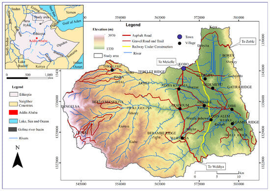
Figure 1.
Location map of Golina River Sub-Basin.
The study area is drained by a dendritic drainage network that includes the east–west-oriented Golina River and its semi-perennial tributaries Hormat and Kelkelit. The sub-basin has a semi-arid climate with maximum temperatures of 18 °C to 30 °C, minimum temperatures of 5 °C to 15 °C, and an average annual temperature of 20 °C. The annual average precipitation of the river sub-basin is about 903 mm [25].
Soil types in the study area include sand, sandy loam, sandy clay, loam, clayey loam, silty clay, and clay soils ([23] and references cited therein). The land use/cover in the basin area is categorized into water bodies, cultivated land, natural forest, shrubland, bare land, and residential lands [23,24].
The outcropping and subsurface lithostratigraphic units that host the primary and most productive aquifers include coarse-grained alluvial deposits composed of sand and gravel and weathered and fractured basaltic rocks, rhyolite, and granites [23,24,25]. The alluvial deposits represent the main aquifer and contain productive layers of sand and gravel. Consequently, most boreholes for domestic and irrigation purposes fetch groundwater from these deposits [23,24,25]. Weathered and fractured basalt rocks in the study area also represent a permeable and productive aquifer. The granites and rhyolites that characterize the eastern part of the study area are impermeable and non-productive [23,24,25].
3. Methods
3.1. Conceptual Model
The groundwater model for any aquifer system begins with the development of a conceptual model to understand the physical framework of the system. This conceptual model describes the natural and anthropogenic factors that contribute to groundwater flow [26]. The conceptual model design for most groundwater flow models should, at a minimum, include boundary information such as hydrostratigraphy and estimates of hydrogeologic parameters, general groundwater flow directions, water sources and sinks, and a field-based groundwater budget [27,28]. The accuracy of the groundwater flow model outputs depends on the accurate representation of the conceptual model.
The driving equations for groundwater flow modeling are based on Darcy’s law [29] and the law of conservation of mass [30]. The three-dimensional groundwater flow with constant fluid density through a heterogeneous and anisotropic porous medium can be described by the following Equation (1):
where Kxx, Kyy, and Kzz are hydraulic conductivity coefficients (L/T) in the x, y, and z directions, respectively; h is the pressure head (L); Ss is the specific storage (1/L); and W is the recharge/discharge rate per unit volume (1/T). The plus sign represents recharge, and the minus sign represents discharge.
The numerical groundwater flow model is designed to solve the equation of groundwater flow through the discretization of space and time. In this study, MODFLOW 6 was used to estimate groundwater flow in the Golina River Sub-Basin. This model was selected because it is easy to understand, use, improve, and modify and is also an open-source program that is freely available [31].
Three-dimensional (3D) numerical groundwater flow modeling of the Golina River Sub-Basin was carried out using the MODFLOW 6 groundwater flow model developed by the U.S. Geological Survey (USGS) [31] and supported by ModelMuse 4, a graphical user interface for MODFLOW 6 [32]. Effective groundwater management requires prediction of subsurface flow and fluid responses to changes in natural and human-induced stresses [3]. Therefore, the numerical groundwater flow model is designed to solve the governing equation of groundwater flow through the discretization of space and time.
To achieve an approximate solution of the groundwater flow equations in aquifer systems, MODFLOW 6 [31] represents the most advanced version of the widely used numerical groundwater flow models. MODFLOW 6 builds on its predecessors and introduces significant improvements in flexibility, modularity, and computational efficiency, making it a powerful tool for groundwater modeling and analysis. In particular, it uses three-dimensional finite-difference methods and is designed to model both steady-state and transient groundwater flows in regional and local aquifer systems.
Hydrological conditions along the boundaries of the conceptual model determine the mathematical boundary conditions of the numerical model, which are crucial to the mathematical model and significantly influence the flow direction, which is calculated by both steady-state and transient numerical groundwater flow modeling. Boundaries include hydraulic features such as groundwater divides and physical features such as surface water bodies and relatively impermeable rocks [27]. The boundary of the model area was delineated using ArcMap 10.8. The surface-water divide is considered a no-flow boundary, i.e., there is no groundwater or surface-water flow between the adjacent river basins (Figure 2 and Figure 3).
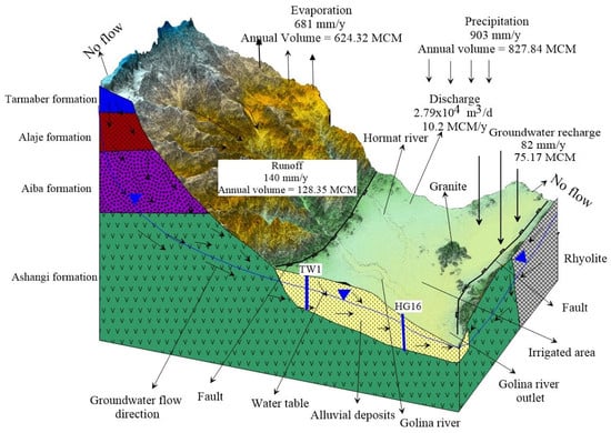
Figure 2.
Conceptual model of the Golina River Sub-Basin.
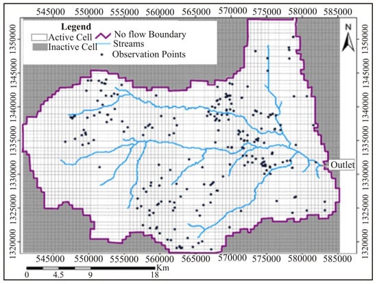
Figure 3.
Discretization and boundary conditions of the model area.
The conceptual model of the Golina River Sub-Basin is constructed based on data-driven lithological logs, geophysical surveys (vertical electrical sounding), pumping tests, and hydrological model results (in this case, WetSpass, modified from [24]). Previous geologic, hydrogeologic, and geophysical surveys and investigations have been carried out to understand the thickness of alluvial sediments and weathered and fractured volcanic rocks in the study area (Figure 2).
Borehole data collected from various water-related governmental and non-governmental organizations provide important information about aquifer parameters, including water levels, discharge rates, total depth, hydraulic conductivity, transmissivity, storativity, and specific yield. Boreholes are concentrated in the alluvial deposits, and in the mountainous areas, there are numerous springs that represent the water level in the tertiary volcanic rocks. The collected data were preprocessed using ArcMap 10.8, Global Mapper 20, and Golden Surfer 16.
3.2. Study Area Modeling and Boundary Conditions
The study area is discretized into 345 rows and 444 columns with a grid size of 100 m by 100 m (Figure 3). It consists of a total of 153,180 cells, with 91,679 active cells and 61,501 inactive cells. Only the active cells were considered for the calculations during model estimation.
The model area comprises two layers: layer-1 represents the alluvial deposit, and layer-2 represents the weathered and fractured volcanic rock (Figure 4). The top elevation of layer-1, the model’s top boundary, is derived from a freely available 12.5 m resolution digital elevation model (DEM) downloaded from www.asf.alaska.edu accessed on 6 April 2023, which was generalized to 100 m resolution for modeling purposes.
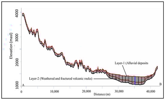
Figure 4.
Model layers and cross-section.
Layer thicknesses were determined from geological logs of boreholes drilled for domestic water supply and irrigation in the Golin River Basin, supported by a geoelectrical survey. The data indicate that the thickness of the alluvial deposits varies from zero near the mountainous area to 272 m at the valley floor’s center, and, to ensure model continuity, a thin synthetic layer of alluvial deposits with a thickness of 0.01 m is assigned to the mountainous area. This assumption has a negligible effect on flow calculations. The thickness of the weathered and fractured volcanic rocks in this model is assigned a constant value of 100 m throughout the valley. The model’s bottom boundary is fresh, compacted, and massive volcanic rock, assumed to be a no-flow bottom boundary, as shown in Figure 3 and Figure 4.
3.3. Model Input Parameters
The crucial input data and parameters of the Golina River Sub-Basin used for the MODFLOW groundwater flow model are the initial hydraulic head; aquifer parameters including hydraulic conductivity [27], transmissivity [21], and specific capacity [33]; recharge and discharge components; drain [31]; and groundwater head observations [34,35].
3.3.1. Initial Hydraulic Head
The static water levels inventory, based on 67 borehole drilling reports and field data collection, has been used to generate the interpolated map of static water level (SWL) for the entire area. The SWL is, therefore, assumed as the initial hydraulic head for the model area, which is one of the key parameters of the groundwater flow model [27].
3.3.2. Aquifer Parameters
Hydraulic conductivity—Hydraulic conductivity of the alluvial deposits showing an eastward gradient ranges from 0.081 to 103.824 m/d. The hydraulic conductivity map has been elaborated with the inverse distance weighting (IDW) interpolation method in ArcMap 10.8, and the average value of the main clastic deposits permitted us to distinguish four different zones (Table 1 and Figure 5).

Table 1.
Hydraulic conductivity (K, m/d) of the alluvial deposits.
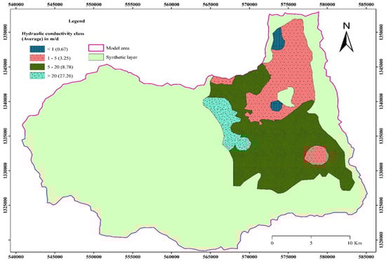
Figure 5.
Hydraulic conductivity map of layer-1 (alluvial deposits) of the study area.
Based on the literature and borehole data from the adjacent Raya Valley [36], which has similar geological characteristics, and taking into account geological and hydrogeological properties of the outcropping units, including their weathering and fracturing degree, the hydraulic conductivity of the weathered and fractured hard rocks ranges from 0.001 to 0.3 m/day (Table 2 and Figure 6).
Table 2.
Hydraulic conductivity (K, m/d) of the weathered and fractured hard rocks.
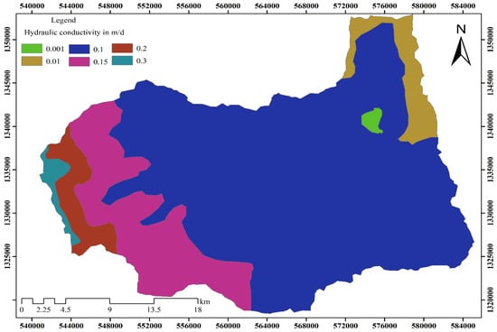
Figure 6.
Initial hydraulic conductivity of layer-2 (weathered and fractured volcanic rocks) of the study area.
Transmissivity—Based on the 67 boreholes reports, the transmissivity of the alluvial deposits permitted us to distinguish boreholes with low (10), medium (36), and high (21) groundwater potential, namely, with values of (5 < T < 50 m2/d), (50 < T <500 m2/d), and (T > 500 m2/d), respectively (Table 3 and Figure 7).
Table 3.
Descriptive statistics of hydraulic parameters for the boreholes in the alluvial aquifer of the Golina River Sub-Basin.
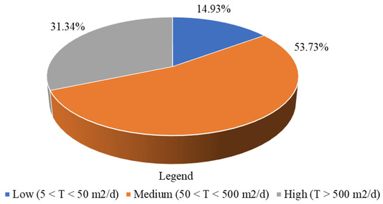
Figure 7.
Percentage of boreholes of the alluvial deposits with low, medium, and high groundwater potential.
Specific capacity—Based on the discharge values of the boreholes ranging from 2.5 to 85 l/s and the drawdowns ranging from 1 to 54.8 m (with an average of 16.64 m), the specific capacity for 64 boreholes varies from 19 m3/d/m to 1077 m3/d/m, with an average of 361 m3/d/m. Taking into account the direct relationship between the specific capacity (SC) and groundwater transmissivity (T) expressed by the following Equation (2),
it turns out that aquifers with high specific capacity, such as alluvial deposits, have a high groundwater potential due to high transmissivity, leading to low drawdown (Figure 8).
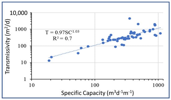
Figure 8.
Transmissivity vs. specific capacity and (log–log plot) for the alluvial aquifer.
3.3.3. Recharge and Discharge
The distribution of groundwater recharge from rainfall was estimated using the WetSpass model [24]. WetSpass provides input to the MODFLOW 6 groundwater flow model via the recharge package boundary condition, which allows the estimation for the Golina River Sub-Basin of an annual groundwater recharge ranging from zero to 1.08 × 10⁻³ m/d, with a mean value of 2.25 × 10⁻⁴ m/d [24].
Groundwater discharge values are derived from pumping test data of boreholes and hand-dug wells, while spring yields are considered negligible. As a result, the total discharges from hand-dug wells and boreholes for water supply and irrigation are estimated to be 2.79 × 10⁴ m3/d, equivalent to 10.2 × 10⁶ m3 per year [24]. In MODFLOW 6, pumping rates are assigned and simulated using Well packages, keeping in mind that the resulting values for groundwater extraction are always negative.
3.3.4. Drain
The drainage package in MODFLOW 6 simulates the effect of removing groundwater from the aquifer at a rate proportional to the difference between the head in the aquifer and fixed head or elevation, called drainage elevation, provided that the head in the aquifer exceeds that elevation [31].
The constant of proportionality is known as the drain conductance, and the flow rate from the aquifer into the drain is calculated using the following Equation (3):
where Q is the flow from the aquifer into the drain (L3T−1), C is the drain conductance (L2T−1), h is the head in the cell containing the drain or aquifer hydraulic head (L), d is the drain elevation (L), K is the hydraulic conductivity of the drain material, L is the length of the drain within the cell (L), W is the width of the stream within the cell (L), and M is the thickness of streambed material (L).
Because there is no river inflow from nearby catchments into the study area, the Drain package was used in this model to estimate the amount of water that leaves the aquifer system. All waters with heads above 5 m below the ground surface are considered drains from the aquifer system, which mainly represent the rivers, springs, and swampy waters [34]. This head (drain) elevation represents water loss through rivers, springs, wetlands, and other surface water bodies [34]. An initial drain conductance value of 100 m2/d was used for each model cell, which was later adjusted during the calibration process to a calibrated value of 200 m2/d.
3.4. Groundwater Head Observations
Measurements of groundwater head from boreholes, hand-dug wells, and springs were conducted throughout the data collection period from 2016 to 2019 (Figure 9). The pumping and monitoring wells in the study area were sealed and lacked observation pipes in some cases, which made it challenging to measure the groundwater head in these wells. The head measurements of springs and hand-dug wells in the weathered and fractured volcanic rocks (layer-2) were used for model calibration. Additionally, the static water levels of boreholes in alluvial deposits (layer-1) recorded during drilling were utilized.
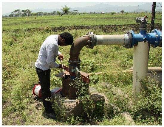
Figure 9.
Groundwater level measurement using the deep meter in Golina River Sub-Basin.
A total of 160 observation points were used for model calibration. MODFLOW 6 includes a flexible new observation (OBS) capability for defining various types of observations. This capability does not support the specification of field-measured observations, calculation of residuals, or interpolation within a grid, as supported in previous MODFLOW versions [31]. The simulated observation heads are output as a file with the extension “.ob_gw_out_head” in Microsoft Excel 2016comma-separated value format. These results are further processed in Excel 2016 software to calculate residual errors, mean absolute errors, and root mean squares.
4. Results and Discussion
4.1. Model Sensitivity Analysis
The primary purpose of the sensitivity analysis was to understand how changes in specific parameters (e.g., hydraulic conductivity, recharge, and well withdrawal) affect the calibrated model output (e.g., simulated head).
The sensitivity of a particular parameter was determined by setting all calibration parameters to their calibrated values except for the selected parameter, which was varied in successive forward runs of the model by increasing and decreasing its value by a specified percentage from its calibrated value [27].
This was conducted by observing changes in the root-mean-square error in response to variations in the selected parameters. The sensitivity analysis was performed by increasing (by 25%, 50%, and 75%) and decreasing (by −25%, −50%, and −75%) the hydraulic parameters and analyzing the corresponding RMSE results of the calibrated model. The analysis revealed that the model is highly sensitive to the hydraulic conductivity of the aquifers, moderately sensitive to recharge, and less sensitive to well abstraction within the model area. Furthermore, recharge was also found to have a higher sensitivity than the other parameters when the changed parameters decreased by −50% and 75% (Figure 10). The model exhibits high sensitivity to hydraulic conductivity due to the heterogeneity of the formations resulting from variations in the fractured permeability of the volcanic rocks across the study area. The moderate sensitivity to recharge, as the distribution of recharge is uneven throughout the river basin, is influenced by variations in fracture interconnectivity. The lower sensitivity to the pumping rate is primarily because pumping wells are concentrated in the alluvial deposit aquifers relatively homogenously, which have a high specific yield.
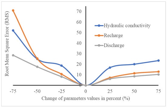
Figure 10.
Model sensitivity analysis.
During the sensitivity analysis, the hydraulic head exhibited significant changes with variations in hydraulic conductivity and recharge compared to other parameters (Figure 10). The response of the aquifer system to increases in hydraulic conductivity was more pronounced than that to increases in other parameters, and the decrease in recharge showed a significant impact, similar to the hydraulic conductivity. This indicates that the hydraulic head of the study aquifer system in the study area is particularly sensitive to climate change.
4.2. Model Calibration
Model calibration is another key step in groundwater flow modeling. It is addressed to make robust and reliable the parameters of the model. The goal of model calibration is to adjust the model parameters so that the simulated results match the field conditions, such as water levels at wells, within acceptable error limits [37].
In this study, the primary target of the calibration was the hydraulic head of selected wells (N = 160), which permitted us to reconstruct the piezometric surface of the Golina River Sub-Basin. Both observed and simulated heads of the selected wells were used for calibration.
Model calibration involves adjusting the model parameters within their expected ranges until the difference between the simulated and observed heads is minimized. This difference is called the residual error (hm—hs). The objective is to match the simulated heads with the observed heads by adjusting the relevant aquifer parameters. A well-calibrated model is characterized by resulting low residual errors.
A manual trial-and-error calibration method was used in this study [27]. The model was repeatedly run by modifying the hydraulic conductivity of the aquifer layers until the simulated heads matched the observed heads. Scatter plots were used to compare observed and simulated heads, and the correlation coefficient (r2) was calculated to assess the fit. The scatter plot showed that the wells were closely aligned with the 1:1 line, with a high correlation coefficient (r2 = 0.998), indicating that the model was well-calibrated (Figure 11). Following [27], summary statistics of the average between the observed and simulated head were calculated to assess model accuracy using the following equations.
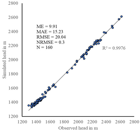
Figure 11.
Scatter plot of observed and simulated heads.
Mean error (ME) is the mean difference in the residual errors and is very important for reducing biases to fit the model:
where ME is the mean error, hm is the field-observed (measured) head (m), hs is the model-simulated head (m), and n is the number of observation points used for model calibration.
Mean absolute error (MAE) is the absolute value of the residual error of the selected wells, and it is larger than the mean error and a better indicator of model fit:
where MAE is the mean absolute error, hm is the field-observed (measured) head (m), hs is the model-simulated head (m), and n is the number of observation points used for calibration.
Root-mean-square error (RMSE) is the square root of the average of the squared residuals, offering a measure that is sensitive to large errors:
where n is the number of selected wells for calibration, hm is the measured or observed head of the wells, and hs is the model-simulated head of the wells.
The residual errors ranged from −63 to 69 m, with 89% of observations falling within the range of −19 to 36 m (Figure 12). The ME, MAE, and RMSE calculated values were 9.91 m, 15.23 m, and 20.04 m, respectively (Figure 11). In addition, due to the large variation in the observed head values, the model accuracy was evaluated using the normalized root-mean-square error (NRMSE). The average normalized RMSE was approximately 0.3 (Figure 11).
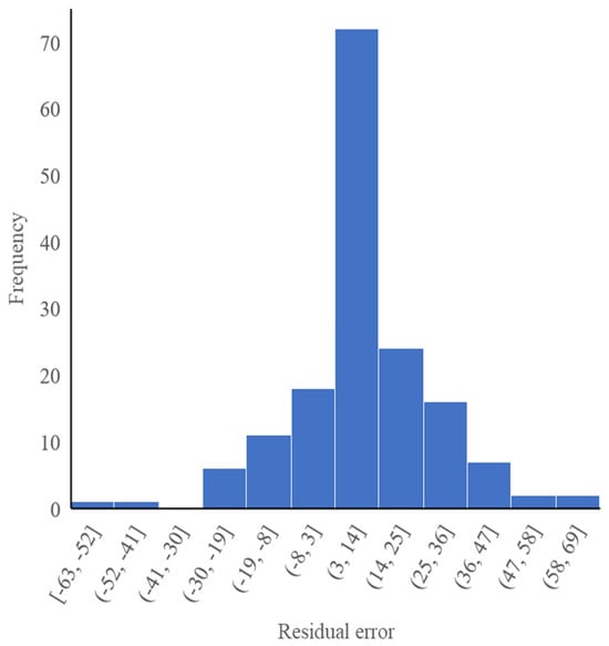
Figure 12.
Frequency distribution of groundwater head residuals.
The residual errors of the mountainous area characterized by weathered and fractured magmatic rocks exhibited large positive values, indicating an underestimation of the groundwater level by the model. And the high residual errors in the weathered and fractured volcanic rocks (layer-2) are attributed to the heterogeneous properties of the formation. Negative residual errors were observed around rivers and streams in mountainous areas, indicating an overestimation of the groundwater levels. The residual errors for the valley floor covered with alluvial deposits are smaller positive errors, which suggests that there was an underestimation of the groundwater level by the model. And the low residual errors observed in the alluvial deposits (layer-1) are related to the homogeneity of the aquifer formations.
The calibrated hydraulic conductivity varied from a minimum of 1.2 × 10⁻⁴ m/day for the impermeable rhyolite to a maximum of 20 m/day for gravel-dominated alluvial deposits (Table 4 and Figure 13 and Figure 14). The calibrated horizontal hydraulic conductivity is much lower than the measured hydraulic conductivity that was measured from the pumping tests, which may be due to the fact that the groundwater wells were located in locations where the materials are productive.
Table 4.
Calibrated horizontal hydraulic conductivity (Kh) of the groundwater flow model layers.
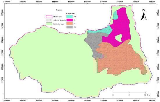
Figure 13.
Calibrated hydraulic conductivity of layer-1 zones (alluvial deposits).
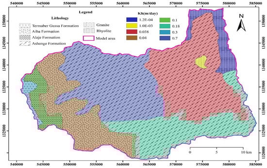
Figure 14.
Calibrated horizontal hydraulic conductivity of layer-2 zones (weathered and fractured volcanic rocks).
4.3. Simulated Groundwater Head and Flow Direction
According to the simulated hydraulic head map generated by the model (Figure 15), the highest simulated groundwater head was observed in the western part of the Golina River Sub-Basin. The lowest-value simulated groundwater head was found toward the outlet at the eastern part of the Golina River Sub-Basin. According to the simulated groundwater head map generated by the model, groundwater flows toward the east of the river basin from all directions. The simulated groundwater head contours are closely spaced in the mountainous areas, indicating a large hydraulic-head gradient, and the contours on the valley floor are widely spaced, indicating a smaller hydraulic-head gradient.
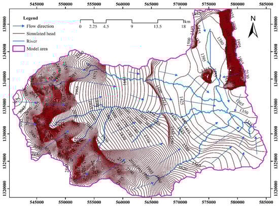
Figure 15.
Simulated head with 15 m contour interval and flow direction.
The findings of this model indicate that the central, western, and eastern parts of the river basin are characterized by the proximity of the contours, the large hydraulic-head gradient of the groundwater, and the significant residual errors due to the rugged topography and steep slopes. Additionally, a hydrogeological map of the study area was created by integrating the lithologies, hydraulic conductivity, water points (including boreholes, hand-dug wells, and springs), streams, and simulated hydraulic heads, as shown in Figure 16.
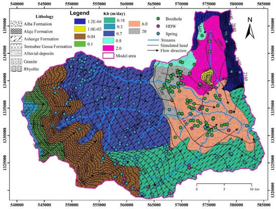
Figure 16.
Hydrogeological map of the Golina River Sub-Basin.
4.4. Water (Volumetric) Budget of the Model Area
The water budget (balance) summarizes all inflows (sources) and outflows (sinks) of water in the groundwater flow model. Under a calibrated steady-state model, the difference between inflows and outflows should be zero or close to zero. The water budget analysis indicates that a total water volume of 207,775.8297 m3/day enters (recharge) the groundwater system while 207,775.9373 m3/day exits (drain) the system under the assumed steady-state groundwater flow modeling of the study river basin (Table 5). The difference between the inflow and outflow is −0.1076 m3/day, as shown in Table 5. The percentage discrepancy is effectively zero, indicating that the model is operating under steady-state conditions. Consider that precipitation is the only source of inflow to the groundwater system and that drain discharge and pumping are the mechanisms through which water outflows. The negative deviation and percentage discrepancy show that the volume of water drained and fetched from the groundwater system is slightly larger than that of the water feeding the aquifer. Groundwater outflow through the drain accounts for about 86.55%, while about 13.45% is due to well abstractions for domestic water supply and irrigation.
Table 5.
Water budget in m3/day of the assumed steady-state model.
4.5. Scenario Analysis
The purpose of developing a steady-state groundwater flow model was to predict possible future changes in groundwater heads due to increased groundwater extraction for different activities and to estimate the impacts of climate change in the study area. Two scenario analyses were used to understand their effect on the aquifer systems of the study area. The first scenario aimed to observe the consequences related to the diffusion of ongoing irrigation projects in the study area, simulated with the increasing of the pumping rate by 25, 50, and 75%. The second scenario was aimed at understanding the effects induced by the decreased rainfall that is occurring throughout the region due to climate change, which is causing a decrease in the aquifer recharging of 25, 50, and 75%.
4.5.1. Effect of Increasing Pumping Rates
To observe the response of the aquifer system, particularly in the currently active irrigation areas, the pumping rates were increased by 25%, 50%, and 75%. When the well-pumping rate was increased by 25%, the volumetric discharge rate increased from 27,945.20 m3/day (Table 5) to 34,931.51 m3/day (Table 6), a difference of 6986.31 m3/day. This increase of 6986.31 m3/day induced a decline in the hydraulic head of 4.64 m. When the well-pumping rates increased by 50% and 75%, the discharge rates increased by 13,972.62 m3/day and 20,958.93 m3/day, respectively. Consequently, the average decline in the groundwater level was 10.18 m for a 50% increase and 17.38 m for a 75% increase.
Table 6.
Water balance of the model induced by an increase in pumping flow rate of 25%, 50%, and 75%.
This scenario had impacts not only on the groundwater level but also on other volumetric budget components, such as water loss through the drain. Furthermore, when the pumping rate was increased by 25%, 50%, and 75%, the volume of the drain water decreased from 179,830.73 m3/day (Table 5) to 172,844.48 m3/day, 165,858.15 m3/day, and 158,871.99 m3/day, respectively, as shown in Table 6.
4.5.2. Effect of Decreasing Recharge
The second scenario included a reduction in the groundwater recharge of the aquifer system of 25%, 50%, and 75%. For a 25% reduction in recharge, the average hydraulic head decreased (declined) by 6.00 m across the model. The most significant decline in the hydraulic head was observed in layer-2 (weathered and fractured volcanic rocks) compared to layer-1 (alluvial deposits). A 50% and 75% reduction in the groundwater recharge resulted in an average decline in the hydraulic head of 15.29 m and 46.97 m, respectively. Therefore, the impacts of decreased recharge were more pronounced in the weathered and fractured aquifer than in the alluvial deposits. Similarly, the reduced groundwater recharges in the study area also affected the volume of water leaving the aquifer system through drain, as shown in Table 7.
Table 7.
Water balance of the model induced by aquifer recharge flow reduction of 25%, 50%, and 75%.
The variation in groundwater recharge in the Golina River Sub-Basin has significant implications for the sustainable use of groundwater resources, especially during drought periods resulting from climate change [35]. This variation affects the water level in the aquifer and also the components of the outflows and can potentially harm the entire ecological system of the Golina River Sub-Basin. The influence of fluctuations in groundwater recharge on the hydraulic head is significantly greater compared to changes in pumping rates, especially when the groundwater recharge decreases by 75%. The results of this scenario analysis indicate that targeted efforts to increase groundwater recharge in the Golina River Sub-Basin are needed to ensure sustainable water resource development and management.
5. Conclusions and Recommendations
5.1. Conclusions
A steady-state numerical model of groundwater flow in the Golina River Sub-Basin was developed to analyze the response of the aquifer to various scenarios induced by anthropogenic activities and climate changes. The model simulated using MODFLOW 6 discretized the study area into a grid of 345 rows and 444 columns for a total of 153,180 cells, of which 91,679 are active.
The model includes two lithostratigraphic layers: the upper clastic layer with a thickness of 272 m (alluvial valley) to 0.01 m (in the mountainous area) and a weathered and fractured hard-rock lower layer with a thickness of 100 m. Assumptions made in the model include (1) a no-flow boundary on the water divide with adjacent basins; (2) groundwater recharge and pumping rates as specific flux boundary conditions; and (3) a drain package assigned as a head-dependent flux for head elevation greater than 5 m below the ground surface. Initial hydraulic conductivity values ranged from 0.001 m/day for rhyolite to 27.26 m/day for alluvial deposits.
The results show that the model is very sensitive to changes in hydraulic conductivity, moderately sensitive to recharge, and less sensitive to well-pumping rates. Although further improvements could be made, the model provides an initial estimate of the difference between the total volume of the groundwater recharge of the aquifer (207,775.8297 m3/day) and the total volume that can be withdrawn under steady-state conditions (207,775.8297 m3/day), with a difference of −0.1076 m3/day and zero-percent discrepancy.
Using the valid model, increased groundwater pumping rates and decreased groundwater recharge were tested. An increase in groundwater pumping rates of 25%, 50%, and 75% results in a decline in the groundwater level by 4.64 m, 10.18 m, and 17.38 m, respectively. Decreasing the groundwater recharge by 25%, 50%, and 75% leads to greater declines in the groundwater level by 6 m, 15.29 m, and 46.97 m, respectively. The largest effects of increased pumping rates were observed in the upper layer (alluvial deposits), and the largest effects of reduced groundwater recharge were observed in the lower layer (weathered and fractured bedrocks). Scenario analyses suggest that changes in groundwater pumping and recharge also affect other components of the aquifer system outflow, such as drainage.
There is still much work to be done to improve the model, and, although the model is not yet ready to be used for management purposes, with this work, the most important decision-makers and stakeholders will be able to understand that its reliability and, therefore, its usefulness require that for a sufficiently long period, the following recommendations are accepted and respected.
5.2. Recommendations
- ⮚
- It is recommended to carry out field studies to accurately assess the hydraulic conductivity of layer-2 in particular, because the current values are based on the scientific literature, and to improve those of layer-2.
- ⮚
- Establish a network of representative municipality and community stakeholders to monitor groundwater levels and estimate abstraction rates in representative wells in the sub-basin, particularly those used for extensive/intensive irrigation. This includes ensuring that wells are accessible for periodic groundwater-level measurements and that selected wells have reliable contactors that measure withdrawals.
- ⮚
- Similarly, identify river-level measuring stations at different locations along the Hormat, Golina, and Kelkelit rivers and at the mouth of the Golina River Sub-Basin and install fixed and portable instrumentation to accurately measure the flows of these rivers.
- ⮚
- Given the observed reduction in aquifer recharge and its impact on groundwater levels, based on the results obtained, it is urgent to develop recommendations and guidelines for the monitoring and sustainable management of wells, especially those used for agriculture, which are the ones that contribute most to the overexploitation of the aquifers.
- ⮚
- It is, therefore, recommended that decision-makers, water resource managers, and researchers, based on data already collected and those that will be collected periodically at the beginning and end of the dry session, contribute (1) to the modeling of groundwater flow under transient conditions (the researchers) and (2) to the optimization and strengthening of the capacity for sustainable management of the groundwater resources in the study area (the resource managers).
Author Contributions
Conceptualization, H.G. and T.G.; methodology, H.G., T.G. and E.H.; software, H.G.; validation, H.G., T.G. and E.H.; formal analysis, H.G. and T.G.; investigation, H.G., T.G., E.H. and N.P.; resources, H.G.; data curation, H.G.; writing—original draft preparation, H.G.; writing—review and editing, T.G., E.H. and N.P.; visualization, H.G. and T.G.; supervision, T.G. and E.H.; project administration, H.G.; funding acquisition, H.G. and T.G. All authors have read and agreed to the published version of the manuscript.
Funding
This research received no external funding.
Data Availability Statement
The data are available from the corresponding author upon reasonable request.
Acknowledgments
The authors wish to thank Samara University, Mekelle University, and the Technical University of Darmstadt (TUD) for supporting this research. We also extend our appreciation to the Ministry of Water, Irrigation, and Electricity of Ethiopia, the Kobo-Girana Valley Development Program Office (KGVDPO), and the Water Resource Office of Kobo Woreda for providing essential information and supporting us during the fieldwork data collection.
Conflicts of Interest
The authors declare that there are no conflicts of interest.
References
- Freeze, R.A.; Cherry, J.A. Groundwater. In Groundwater; The Groundwather Foundation: Westerville, OH, USA, 1979. [Google Scholar]
- Singhal, B.B.S.; Gupta, R.P. Applied Hydrogeology of Fractured Rocks: Second Edition; Springer: Berlin/Heidelberg, Germany, 2010; ISBN 978-90-481-8798-0. [Google Scholar]
- Cushman, J.H.; Tartakovsky, D.M. The Handbook of Groundwater Engineering: Third Edition; Routhledge: Abingdon, UK, 2016; ISBN 978-1-4987-0305-5. [Google Scholar]
- Hu, B.X.; Wu, J.; He, C. On Stochastic Modeling of Groundwater Flow and Solute Transport in Multi-Scale Heterogeneous Formations. Comput. Appl. Math. 2004, 23, 121–152. [Google Scholar] [CrossRef][Green Version]
- Zektser, I.S.; Everett, L.G. Groundwater Resources of the World and Their Use; Unesco: Paris, France, 2004; ISBN 92-9220-007-0. [Google Scholar]
- Azeref, B.G.; Bushira, K.M. Numerical Groundwater Flow Modeling of the Kombolcha Catchment Northern Ethiopia. Model. Earth Syst. Environ. 2020, 6, 1233–1244. [Google Scholar] [CrossRef]
- Rossman, N.R.; Zlotnik, V.A. Review: Regional Groundwater Flow Modeling in Heavily Irrigated Basins of Selected States in the Western United States. Hydrogeol. J. 2013, 21, 1173. [Google Scholar] [CrossRef]
- Senent-Aparicio, J.; Peñafiel, L.; Alcalá, F.J.; Jimeno-Sáez, P.; Pérez-Sánchez, J. Climate Change Impacts on Renewable Groundwater Resources in the Andosol-Dominated Andean Highlands, Ecuador. Catena 2024, 236, 107766. [Google Scholar] [CrossRef]
- Varalakshmi, V.; Venkateswara Rao, B.; SuriNaidu, L.; Tejaswini, M. Groundwater Flow Modeling of a Hard Rock Aquifer: Case Study. J. Hydrol. Eng. 2014, 19, 877–886. [Google Scholar] [CrossRef]
- Yihdego, Y.; Danis, C.; Paffard, A. 3-D Numerical Groundwater Flow Simulation for Geological Discontinuities in the Unkheltseg Basin, Mongolia. Environ. Earth Sci. 2015, 73, 4119–4133. [Google Scholar] [CrossRef]
- Yihdego, Y.; Webb, J.A.; Leahy, P. Modelling of Lake Level under Climate Change Conditions: Lake Purrumbete in Southeastern Australia. Environ. Earth Sci. 2015, 73, 3855–3872. [Google Scholar] [CrossRef]
- Razack, M.; Furi, W.; Fanta, L.; Shiferaw, A. Water Resource Assessment of a Complex Volcanic System under Semi-Arid Climate Using Numerical Modeling: The Borena Basin in Southern Ethiopia. Water 2020, 12, 276. [Google Scholar] [CrossRef]
- Ahmed, S.; Jayakumar, R.; Salih, A. Groundwater Dynamics in Hard Rock Aquifers: Sustainable Management and Optimal Monitoring Network Design; Springer: Berlin/Heidelberg, Germany, 2008; ISBN 978-1-4020-6539-2. [Google Scholar]
- Meyer, P.A.; Brouwers, M.; Martin, P.J. A Three-Dimensional Groundwater Flow Model of the Waterloo Moraine for Water Resource Management. Can. Water Resour. J. 2014, 39, 167–180. [Google Scholar] [CrossRef]
- Pétré, M.A.; Rivera, A.; Lefebvre, R. Numerical Modeling of a Regional Groundwater Flow System to Assess Groundwater Storage Loss, Capture and Sustainable Exploitation of the Transboundary Milk River Aquifer (Canada, USA). J. Hydrol. 2019, 575, 656–670. [Google Scholar] [CrossRef]
- Islam, M.B.; Firoz, A.B.M.; Foglia, L.; Marandi, A.; Khan, A.R.; Schüth, C.; Ribbe, L. A Regional Groundwater-Flow Model for Sustainable Groundwater-Resource Management in the South Asian Megacity of Dhaka, Bangladesh. Hydrogeol. J. 2017, 25, 617–637. [Google Scholar] [CrossRef]
- Michael, H.A.; Voss, C.I. Controls on Groundwater Flow in the Bengal Basin of India and Bangladesh: Regional Modeling Analysis. Hydrogeol. J. 2009, 17, 1561–1577. [Google Scholar] [CrossRef]
- Zhou, Y.; Li, W. A Review of Regional Groundwater Flow Modeling. Geosci. Front. 2011, 2, 205–214. [Google Scholar] [CrossRef]
- Janos, D.; Molson, J.; Lefebvre, R. Regional Groundwater Flow Dynamics and Residence Times in Chaudière-Appalaches, Québec, Canada: Insights from Numerical Simulations. Can. Water Resour. J. 2018, 43, 214–239. [Google Scholar] [CrossRef]
- Desalegn, A. Groundwater Potential Evaluation and Flow Dynamics of Hormat, Golina River Catchment, Kobo Valley, North Ethiopia. Master’s Thesis, Addis Ababa University, Addis Ababa, Ethiopia, 2011. [Google Scholar]
- Tadesse, M.; Bekele, H.; Mitiku, B.; Teshome, M.; Besufekade, A.; Edris, M.; Burussa, G.; Yehualaeshet, E.; Alemu, S.; Tadesse, A. Geology, Geochemistry and Gravity Survey of the Maychew Area: Memoir 31; Ministry of Mines, Geological Survey of Ethiopia, Basic Geoscience Mapping Core Process: Addis Ababa, Ethiopia, 2011; p. 68.
- Tadesse, N.; Nedaw, D.; Woldearegay, K.; Gebreyohannes, T.; Steenbergen, F.V. Groundwater Management for Irrigation in the Raya and Kobo Valleys, Northern Ethiopia. Int. J. Earth Sci. Eng. 2015, 8, 1104–1114. [Google Scholar]
- Gebru, H.; Gebreyohannes, T.; Hagos, E. Identification of Groundwater Potential Zones Using Analytical Hierarchy Process (AHP) and GIS-Remote Sensing Integration, the Case of Golina River Sub-Basin, Northern Ethiopia. Int. J. Adv. Remote Sens. GIS 2020, 9, 3289–3311. [Google Scholar] [CrossRef]
- Gebru, H.; Gebreyohannes, T.; Hagos, E. WetSpass Model and Chloride Mass Balance Based Groundwater Recharge Estimation: The Case of Golina River Sub-Basin, Northern Ethiopia. Sustain. Water Resour. Manag. 2023, 9, 188. [Google Scholar] [CrossRef]
- Gebru, H.; Gebreyohannes, T.; Hagos, E. Ascertaining the Source of Major Dissolved Solute and Recharge Mechanism of Groundwater in the Golina River Sub-Basin, Northern Ethiopia. Daagu Int. J. Basic Appl. Res. 2023, 5, 120–143. [Google Scholar]
- Kresic, N.; Mikszewski, A. Hydrogeological Conceptual Site Models: Data Analysis and Visualization; Routhledge: Abingdon, UK, 2013; ISBN 978-1-4398-5228-6. [Google Scholar]
- Anderson, M.P.; Woessner, W.W.; Hunt, R.J. Applied Modeling Groundwater Simulation of Flow and Advective Transport; Elsevier: Amsterdam, The Netherlands, 2015; ISBN 978-0-12-058103-0. [Google Scholar]
- Winter, T.C. The Concept of Hydrologic Landscapes. J. Am. Water Resour. Assoc. 2001, 37, 335–349. [Google Scholar] [CrossRef]
- Darcy, H. Les Fontaines Publiques de La Ville de Dijon. In Recherche; Bnf Site Institutionnel: Paris, France, 1856. [Google Scholar]
- Lavoisier, A.L. Traité Élémentaire de Chimie (Elementary Treatise on Chemistry); Smithsonian Libraries: Paris, France, 1789. [Google Scholar]
- Langevin, C.D.; Hughes, J.D.; Banta, E.R.; Niswonger, R.G.; Panday, S.; Provost, A.M. Documentation for the MODFLOW 6 Groundwater Flow Model; U.S. Geological Survey: Reston, VA, USA, 2017. [CrossRef]
- Winston, R.B. ModelMuse Version 4: A Graphical User Interface for MODFLOW 6; U.S. Geological Survey: Reston, VA, USA, 2019; Volume 10. [CrossRef]
- Chahar, B.R. Groundwater Hydrology; McGraw Hill Education: New Delhi, India, 2015; ISBN 978-93-392-0463-1. [Google Scholar]
- Gebreyohannes, T.; De Smedt, F.; Walraevens, K.; Gebresilassie, S.; Hussien, A.; Hagos, M.; Amare, K.; Deckers, J.; Gebrehiwot, K. Regional groundwater flow modeling of the Geba basin, northern Ethiopia. Hydrogeol. J. 2017, 25, 639–655. [Google Scholar] [CrossRef]
- Balcha, S.K.; Hulluka, T.A.; Awass, A.A.; Bantider, A.; Ayele, G.T.; Walsh, C.L. Numerical Groundwater Flow Modeling under Future Climate Change in the Central Rift Valley Lakes Basin; Ethiopia. J. Hydrol. Reg. Stud. 2024, 52, 101733. [Google Scholar] [CrossRef]
- Bushra, A.H. Quantitative Status, Vulnerability and Pollution of Groundwater Resources in Different Environmental and Climatic Contexts in Sardinia and in Ethiopia. Ph.D. Thesis, University degli Studi di Cagliari, Cagliari, Italy, 2011. [Google Scholar]
- Manghi, F.; Williams, D.; Safely, J.; Hamdi, M.R. Groundwater Flow Modeling of the Arlington Basin to Evaluate Management Strategies for Expansion of the Arlington Desalter Water Production. Water Resour. Manag. 2012, 26, 21–41. [Google Scholar] [CrossRef]
Disclaimer/Publisher’s Note: The statements, opinions and data contained in all publications are solely those of the individual author(s) and contributor(s) and not of MDPI and/or the editor(s). MDPI and/or the editor(s) disclaim responsibility for any injury to people or property resulting from any ideas, methods, instructions or products referred to in the content. |
© 2025 by the authors. Licensee MDPI, Basel, Switzerland. This article is an open access article distributed under the terms and conditions of the Creative Commons Attribution (CC BY) license (https://creativecommons.org/licenses/by/4.0/).