Modeling and Validating Saltwater Intrusion Dynamics by Self-Potential: A Laboratory Perspective

Abstract

Saltwater intrusion (SWI) in coastal aquifers poses a significant threat to freshwater resources, exacerbated by climate change and rising sea levels. This study investigates SWI dynamics using laboratory experiments, geophysical monitoring with the self-potential (SP) method, and numerical simulations to assess the impact of varying salt concentrations (7 g/L and 35 g/L) on intrusion rates and electrochemical responses. Laboratory experiments were conducted in a custom-designed sandbox model, with SP data collected in real time using a 192-electrode system. Numerical simulations were performed to replicate experimental conditions and validate the model’s predictions. Results show that salt concentration significantly influences intrusion rates and SP responses. In low-salinity systems (7 g/L), SP values increased gradually from 0 mV to 20 mV, with a slow intrusion rate of 0.034 m/h. In contrast, moderate-salinity systems (35 g/L) exhibited rapid SP changes (0 mV to 5 mV) and a faster intrusion rate of 0.1 m/h. Sharp SP anomalies near the intrusion source, with values dropping from 10 mV to −40 mV, were observed in low-salinity systems, highlighting localized charge imbalances. The model’s performance was evaluated using relative RMSE, showing a good fit in Experiment (1) (RMSE = 5.00%) and acceptable results for Experiment (2) (RMSE = 23.45%). These findings demonstrate the potential of the SP method for real-time monitoring of SWI and provide insights for improving management strategies in coastal aquifers.

1. Introduction

Coastal aquifers are critical freshwater sources for millions worldwide [1], supporting drinking water, agriculture, and industry [2]. However, these resources are increasingly threatened by SWI [3], where seawater infiltrates freshwater aquifers, forming a saline wedge beneath freshwater. This compromises water quality and availability particularly in regions facing water scarcity [4]. SWI is increasing by over-extraction of groundwater, land-use changes, and climate change, including rising sea levels [5]. The interaction between density and hydraulic gradients drives seawater inland [6,7], often leading to irreversible contamination. Mitigation strategies like artificial recharge and desalination are costly [8], highlighting the need for cost-effective monitoring and management solutions [9,10].

Early research on SWI primarily focused on simplified homogeneous aquifer models. For instance, Henry [11] developed analytical solutions for SWI in idealized homogeneous systems, laying the groundwork for understanding density-driven flow. Later, Voss and Souza [12] advanced numerical modeling techniques to simulate SWI in more complex systems, emphasizing the role of hydraulic conductivity and aquifer heterogeneity. Laboratory experiments have also played a key role in understanding SWI dynamics. For example, Goswami and Clement [13] used sandbox experiments to study the effects of varying salt concentrations and hydraulic gradients on SWI, demonstrating the importance of realistic geological conditions in replicating real-world scenarios. Similarly, Chang and Clement [14] investigated the impact of aquifer heterogeneity on SWI, highlighting how variations in porosity and permeability influence saltwater migration.

Recent studies have further advanced the understanding of SWI using innovative approaches [15,16,17,18,19,20,21,22,23,24,25]. For instance, Folch et al. [26] combined geophysical and hydrogeological methods to monitor SWI in a coastal aquifer in Spain, demonstrating the effectiveness of integrating electrical resistivity tomography (ERT) with groundwater modeling to track saline fronts. Their work highlighted the importance of multi-method approaches for accurate SWI monitoring. Similarly, Cao et al. [5] used a combination of laboratory experiments and numerical simulations of a 2-D SEAWAT model to investigate the effects of sea-level rise and pumping rates on SWI dynamics. Their findings emphasized the need for adaptive management strategies to mitigate the impacts of climate change on coastal aquifers.

Despite these advancements, many studies rely on direct methods such as salinity measurements or visual inspections, which lack precision and real-time monitoring capabilities. Geophysical methods, such as the SP technique, offer a promising alternative. SP measures natural electrical potential generated by ionic movement at the freshwater–saltwater interface, providing real-time, non-invasive monitoring of SWI dynamics. Researchers like Revil et al. [27] have demonstrated the effectiveness of SP in detecting electrochemical gradients associated with SWI, while Graham [28] applied SP in coastal boreholes, combined with a hydrodynamic and electrodynamic model to explain the electrical potential gradient and its reduction prior to SWI. The model highlights the role of electrochemical exclusion and diffusion potentials and suggests that geoelectric heterogeneity controls the SP gradient. This research indicates that borehole SP could potentially serve as an early warning mechanism for SWI.

This research introduces a novel laboratory-scale approach for studying saltwater migration in coastal aquifers through self-potential (SP) monitoring, combined with numerical simulations. This approach provides real-time tracking of SWI dynamics, offering significant advantages over traditional methods such as the ERT and salinity probes, which often lack the spatial density and temporal resolution provided by our 192-electrode system. Recent studies, such as Crestani et al. [29], have demonstrated the value of laboratory experiments for studying SWI, utilizing techniques like ERT to monitor saltwater wedge evolution. However, our method introduces a non-invasive, high-resolution alternative to these traditional methods by using SP measurements to track SWI in real time.

In the work of Stoeckl and Houben [30], sand tank experiments are highlighted as a valuable tool for understanding groundwater flow dynamics in coastal aquifers. Their findings underscore the importance of controlled laboratory settings for investigating complex variable-density flow and transport processes, a framework that supports the application of our SP monitoring technique in studying the dynamics of SWI. Additionally, Yu et al. [31] explored how inland water table changes influence the movement of the saltwater wedge in laboratory-scale unconfined aquifers. This is complementary to our approach, as we also aim to improve the understanding of SWI dynamics in laboratory conditions, but with a focus on SP monitoring for real-time, high-resolution tracking. Furthermore, Sharma and Bhattacharjya [32] investigated contaminant transport within coastal aquifers, showing how the saltwater wedge influences the migration of contaminants. Their research reinforces the need for precise monitoring tools like SP to capture the interaction between saltwater and freshwater zones, which is central to our study.

This research aims to advance our understanding of saltwater migration in coastal aquifers through laboratory-scale experiments integrating SP monitoring with numerical simulations in a novel way. The study introduces an innovative approach by combining laboratory experiments, real-time SP data acquisition using a 192-electrode system, and Particle Swarm Optimization (PSO) to model SWI dynamics. This integration allows for accurate, high-resolution tracking of SWI over time, which is not commonly achieved by traditional methods such as salinity probes and visual inspections. Unlike traditional methods, such as ERT and salinity probes, which often have limitations in spatial density and temporal resolution, our 192-electrode SP system offers high-resolution, continuous monitoring of electrochemical potential variations at multiple electrode positions in real time. This enables a more detailed view of the saltwater–freshwater interface and allows us to track SWI dynamics over time with far greater accuracy than methods like ERT.

For Crestani et al.’s [29] study, they used large-scale physical modeling with ERT to study SWI, demonstrating the value of laboratory experiments for simulating saltwater wedge evolution. While their study provides valuable insights, SP monitoring offers several advantages:

• Higher Spatial Resolution: The 192-electrode system captures real-time data from multiple electrode positions, enabling fine-grained spatial mapping of the saltwater–freshwater interface.
• Real-time Tracking: Unlike ERT, which may require time-consuming data acquisition and analysis, SP monitoring provides continuous, real-time tracking of SWI dynamics, making it more suitable for observing rapid changes in the system.
• Non-invasive Measurement: SP measurements do not require physical contact with the saltwater wedge, offering a non-invasive alternative to salinity probes and visual inspections, which may disturb the system or miss subtle dynamics.

The novelty of this study lies in its integration of experimental data with advanced numerical modeling, utilizing an inclined sheet model for SP calculation to simulate and validate SWI processes. By combining this model with experimental observations, the study offers more reliable predictions for coastal aquifer management. Additionally, it examines how varying salinity levels influence the SWI phenomenon and affect the SP response, providing valuable insights into the role of salinity in SWI dynamics. Furthermore, the study investigates the impact of water level fluctuations on the flow dynamics of SWI and the SP response by applying different hydraulic pressures to simulate sea-level rise.

By simulating these variations and combining them with experimental data, our study enhances the understanding of how environmental changes, particularly changes in flow conditions, influence SWI behavior. This provides a more effective tool for managing coastal aquifers and guiding targeted strategies to mitigate the impacts of SWI, especially in areas impacted by rising sea levels and freshwater scarcity.

2. Materials and Methods

2.1. Laboratory Simulation Setup

A custom-designed experimental apparatus was developed to simulate SWI in a coastal aquifer system. The setup consisted of a steel and glass tank partitioned into three distinct chambers. The central chamber representing a confined aquifer, was filled with homogeneous sand (grain size = 0.425 mm, porosity = 39%) and maintained in a fully saturated state to replicate realistic aquifer conditions. The use of uniform sand ensured that the experiments focused on SWI dynamics without introducing significant heterogeneity, while the chamber dimensions were carefully selected to mimic natural aquifer properties, ensuring consistency with field conditions. To simulate the natural pressure of a confined aquifer, a layer of freshwater was added above the saturated porous medium.

The homogeneous sand was incrementally introduced into the central chamber to minimize air entrapment, which could otherwise disrupt flow dynamics [33]. The central chamber was isolated from the adjacent chambers using fine mesh screens and geotextiles, which prevented the migration of materials between chambers while maintaining controlled experimental conditions as shown in Figure 1.

In the left chamber, freshwater was introduced, while the right chamber was filled with saline water at predetermined concentrations, as outlined in the experimental protocol in

Table 1. Summary of experimental phases and hydraulic conditions.

Phase	Duration	Hydraulic Conditions	Objective
1	0–7 h	Saline water: 47.5 cm Freshwater: 46 cm Interface: 45 cm	Induce right-to-left SWI under a 1.5 cm hydraulic gradient.
2	7–17 h	All chambers equilibrated to 45 cm	Observe steady-state equilibrium and SWI stabilization.
3	17–24 h	Saline water: 46 cm Freshwater: 47.5 cm Interface: 45 cm	Reverse flow direction (left-to-right) to analyze SWI retreat dynamics.

. For Experiment (1), the saltwater concentration was set to 7 g/L, representing the minimum salinity value found in seawater such as in the Baltic Sea [34], where salinity levels are relatively low. For Experiment (2), the saltwater concentration was set to 35 g/L, reflecting the average global seawater salinity [35]. To enhance the visibility of the saline intrusion process [36], red dye was added to the saline solution (McCormick Inc., Shanghai, China, 0.1 mL/L), facilitating the observation of the spatial distribution and intensity of SWI as

Table 2. Key components of the experimental setup.

Component	Specification	Purpose
Central chamber	Homogeneous silica sand (0.425 mm grain size, 39% porosity)	Simulate confined aquifer with controlled hydraulic properties.
Geotextile/mesh barriers (sand filter)	0.1 mm mesh screens + geotextile membranes	Prevent sediment migration between chambers.
Overflow system	Adjustable vertical overflow with drainage pipes	Maintain precise hydraulic heads and evacuate excess water.
Saline water tracer	Red dye (non-reactive)	Visualize SWI progression and spatial distribution.
SP monitoring	SP electrodes + data logger	Measure electrical potentials linked to ionic transport during SWI.

shows.

Water levels in both the freshwater and saline water chambers were regulated using an adjustable overflow system. This system allowed for precise control of water heights, ensuring consistent hydraulic conditions throughout the experiment. Excess water was drained via connected drainage pipes, maintaining accurate water levels within the experimental setup as shown in Figure 2.

The 192-electrode device was placed on top of the saturated sand in the central chamber, as shown in Figure 2, to monitor the SP throughout the experiment. The system captured SP data over a 24 h period, during which the experiment went through the three phases outlined in Table 1. This setup allowed for real-time tracking of the dynamics of SWI across the different experimental conditions.

2.2. Monitoring and Data Acquisition

To monitor SWI dynamics, a comprehensive data acquisition system was employed to capture three-dimensional natural electric potential signals, providing real-time insights into the movement of the freshwater–saltwater interface as shown in Figure 3. The monitoring system comprised the following key components:

2.2.1. Experimental Sandbox Dimensions

The sandbox is designed to simulate aquifer behavior under controlled conditions and measures 130 cm in length, 40 cm in width, and 50 cm in height. These dimensions were selected to provide sufficient space for observing saline water movement while maintaining experimental accuracy.

2.2.2. Data Acquisition Instruments

A 192-channel data acquisition system was utilized, offering a high sampling accuracy of 0.01 mV. This precision enabled continuous, automated data collection throughout the experiment, ensuring accurate measurement of natural electric potential signals in real time.

2.2.3. Electrode Configuration

A three-dimensional array of non-polarized Ag-AgCl electrodes was employed with dimensions of 90 × 30 × 24 cm. The electrodes were uniformly distributed in a 16 × 4 × 3 grid with spacing of 6 × 10 × 12 cm. A total of 192 non-polarized Ag-AgCl electrodes were embedded in an insulated polymer plastic frame, each with a diameter of 6 mm. These button-shaped sintered electrodes were specifically designed for flow potential experiments, enabling the collection of time-sequenced data in three-dimensional space. A reference electrode (Ag/AgCl) was positioned at a fixed location to ensure accurate potential measurements across the system.

2.3. Integration of Monitoring Components

The integration of these components provided a robust and precise monitoring system capable of tracking SWI dynamics in real time. The system facilitated detailed data collection on changes in the freshwater–saltwater interface and associated electrochemical signals, offering a powerful tool for understanding the mechanisms driving SWI. This approach not only enhanced the accuracy of the experimental results but also provided valuable insights for developing predictive models and informing sustainable groundwater management strategies in coastal regions.

By combining controlled laboratory simulations with advanced monitoring techniques, this methodology offers a comprehensive framework for studying SWI dynamics, addressing the limitations of traditional methods and contributing to the development of more effective groundwater management practices.

2.4. Numerical Simulation Methodology

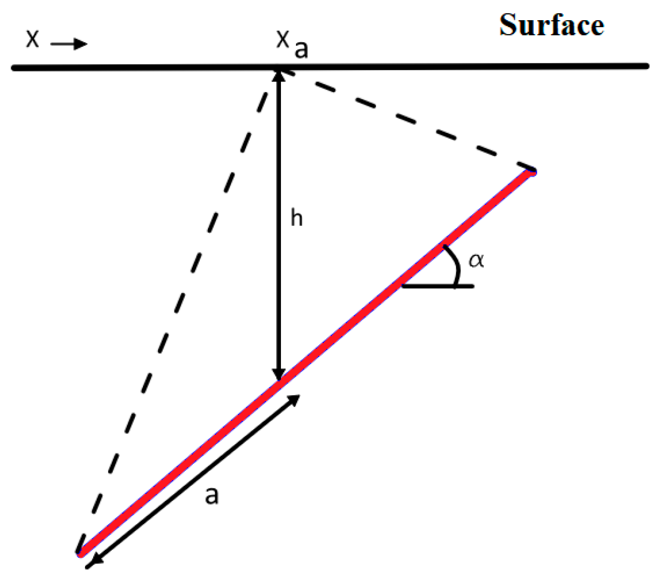
2.4.1. Governing Equations for SP Anomaly

The SP anomaly induced by SWI is modeled using the 2-D inclined sheet model approximation [37,38] shown in Figure 4, which conceptualizes the saline plume as a conductive structure embedded in a homogeneous subsurface medium. The SP distribution V(x) along a linear electrode array is derived from the logarithmic potential equation for a dipolar source:

$$V\left(x\right)=K\ln \left({\displaystyle \frac{{\left(x-x_0-a\cos \alpha \right)}^2+{\left(z-a\sin \alpha \right)}^2}{{\left(x-x_0+a\cos \alpha \right)}^2+{\left(z+a\sin \alpha \right)}^2}}\right) ,$$

(1)

where

• K (mV·m) is the electric dipole moment, proportional to salinity contrast and ionic mobility.
• $x_0$ (m) is the horizontal position of the sheet’s geometric center.
• z (m) is the depth to the sheet’s center.
• α (°) is the polarization angle (inclination of the saline plume relative to the horizontal).
• a (m) is the half-length of the sheet.

Figure 4. Explanation of 2-D inclined sheet model parameters.

Figure 4. Explanation of 2-D inclined sheet model parameters.

This equation quantifies the spatial decay of the SP signal as a function of distance from the source, modulated by the sheet’s geometry and orientation.

2.4.2. Data Preprocessing

(a)

Baseline Correction:

To isolate transient SP signals caused by saline intrusion, the baseline measurement at $t=0$ is subtracted from subsequent time steps:

$$V_{adjusted }\left(t,x\right)=V_{measured }\left(t,x\right)-V_{measured }\left(0,x\right).$$

(2)

• (b) Noise Reduction:

A moving average filter with a window size W = 5W = 5 is applied to suppress high-frequency noise:

$$V_{smoothed }\left(t,x\right)={\displaystyle \frac{1}{W}} \sum _{i=-2}^2{V}_{adjusted }\left(t,x+i\mathrm{\Delta }x\right),$$

(3)

where $∆\left(x\right)=0.1 \mathrm{m}$ is the inter-electrode spacing.

2.4.3. Data Inversion with Particle Swarm Optimization (PSO)

The parameters of the inclined sheet $(K, x_0, z, \alpha , a)$ are estimated using PSO, a global optimization algorithm [37].

(a)

Objective Function:

The root mean squared error (RMSE) between measured and modeled SP data is minimized, with a penalty term enforcing V ≈ 0 at t = 0:

$$\mathrm{R}\mathrm{M}\mathrm{S}\mathrm{E}=\sqrt{{\displaystyle \frac{1}{N}}\sum _{j=1}^N{{(V}_{smoothed,j}-V_{model,j}\left(x_i\right))}^2}+\lambda .\left|{\displaystyle \frac{1}{N}}\sum _{j=1}^N{V}_{model,j}\left(x_i\right)\right| ,$$

(4)

where λ = 500 penalizes deviations from baseline conditions, and N = 16 is the number of electrodes of each horizontal line in the 3D electrode model device.

(b)

Search Space Constraints:

Parameter bounds are defined to reflect site-specific constraints for saline intrusion:

$$Kϵ\left[-20, 20\right], x_0ϵ\left[0, 1\right], zϵ\left[0, 0.5\right], \alpha ϵ\left[0°, 180°\right], aϵ\left[0, 1\right]$$

(c)

PSO Algorithm:

• Swarm Initialization: 100 particles are randomly initialized within the search space.
• Velocity and Position Update:

$$v_i^{\left(t+1\right)}=\omega v_i^{\left(t\right)}+c_1{r}_1\left(P_{best,i}-x_i^t\right)+c_2{r}_2\left(g_{best,i}-x_i^t\right) ,$$

(5)

$$x_i^{(t+1)}=x_i^{\left(t\right)}+v_i^{(t+1)},$$

(6)

• where $\omega =0.5$ (inertia weight), $c_1=c_2=2.0$ (cognitive/social coefficients), and $r_1,r_{2 }~ U\left(0, 1\right).$

• Termination: The algorithm terminates after 200 iterations or upon convergence (stagnation in $g_{best}$).

2.4.4. Validation and Performance Metrics

(a)

Quantitative Validation:

-

RMSE: Evaluates the fit between measured and modeled SP data.

-

Parameter Stability: Consistency of optimized parameters across independent PSO runs.

(b)

Noise Tolerance:

Synthetic datasets with 10–20% Gaussian noise are inverted to assess robustness.

(c)

Visual Verification:

Overlays are generated to qualitatively validate the fit.

2.4.5. Boundary Conditions

The numerical model used to simulate the SWI process also incorporated boundary conditions that reflected the experimental setup. In the numerical model, the boundaries were defined by the freshwater–saline water interface, and the movement of this interface was tracked over time. The boundaries for both saline and freshwater chambers were represented as regions where the concentration and flow properties were defined based on the experimental settings.

The following conditions were applied:

-

The left boundary (x = 0) represented the freshwater chamber, where freshwater was introduced.

-

The right boundary (x = 1) represented the saline water chamber, where saline water was added.

-

The interface (middle chamber) between the freshwater and saline water was modeled as the primary dynamic boundary, moving over time due to the induced hydraulic gradient and changes in water levels according to the experimental protocol in Table 1.

These boundary conditions were critical in simulating the progression of SWI and accurately calculating SP using the 2-D inclined sheet model. The numerical solution was implemented using MATLAB R2017a software, where custom scripts were developed to calculate the SP values at each electrode position. The movement of the interface and the resulting SP values were then used to validate the model by comparing the calculated SP to the experimentally measured SP values.

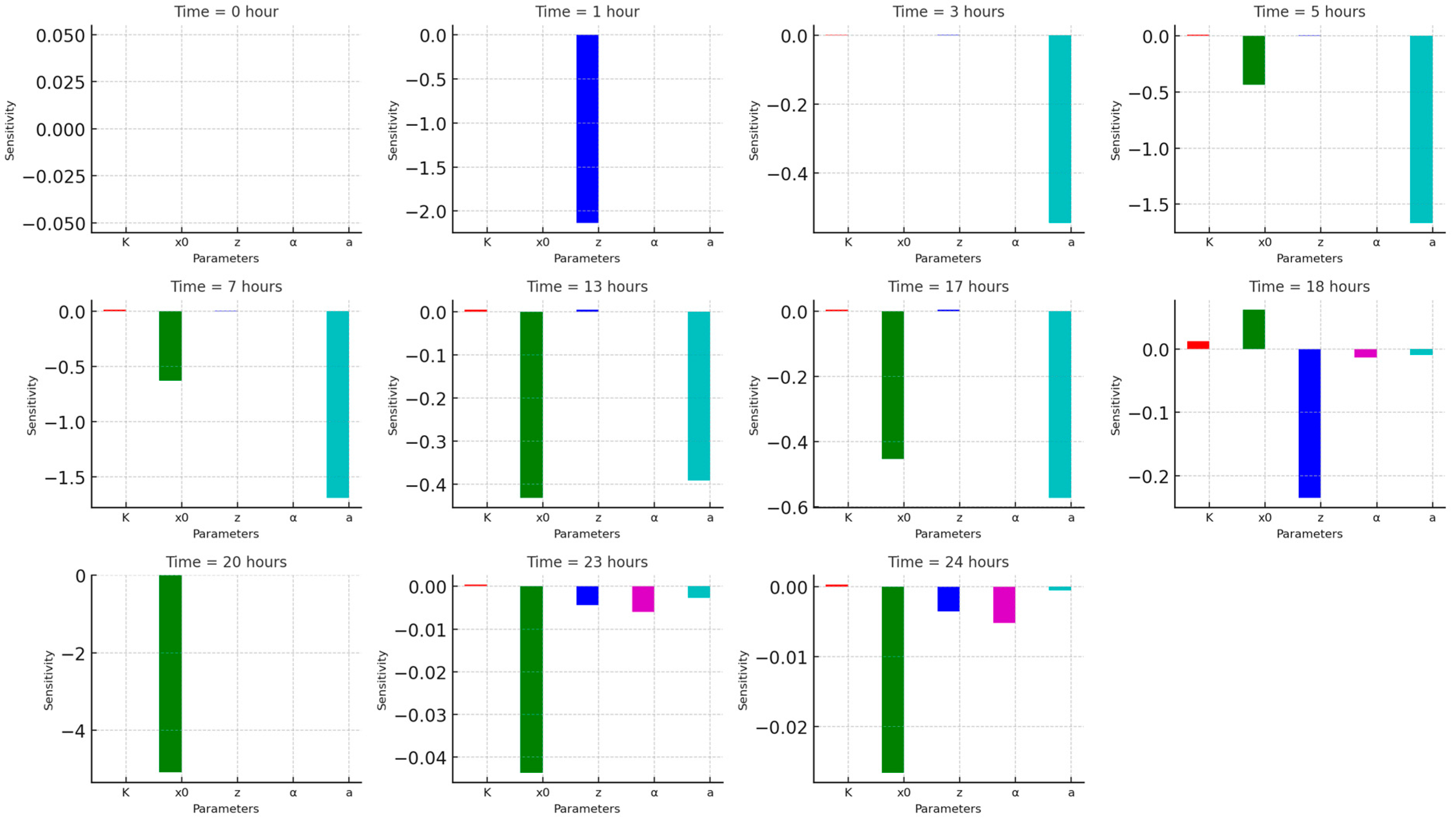
2.4.6. Sensitivity Calculation

The sensitivity analysis was conducted to quantify how changes in the model parameters influence the simulated SP values using central difference approximation across different time steps [39]. The model parameters under investigation include the five parameters of the 2-D inclined sheet model: K, x0, z, α, and a. To perform the sensitivity analysis, the following approach was used:

(a)

Perturbation of Parameters: Each parameter was individually perturbed by ±1% of its original value, creating two sets of perturbed parameters: one set with an increased value (+1%) and one set with a decreased value (−1%). This perturbation was applied to each of the five parameters: K, x0, z, α, and a.

(b)

Objective Function Evaluation: For each perturbed set of parameters, the objective function was evaluated. The objective function compares the measured SP values with the simulated SP values and calculates the root mean squared error (RMSE) between the two. The error was computed for both the perturbed (+1%) and the reduced (−1%) parameter values.

(c)

Sensitivity Calculation: The sensitivity of each parameter was calculated using the following formula:

$$Sensitivity={\displaystyle \frac{{Error}_{+1\%}-{Error}_{-1\%}}{2\times Perturbation\times Original Value}}$$

(7)

Here, Error_+1% and Error_−1% represent the RMSE values for the perturbed parameters, and Original Value is the baseline parameter value. This formula provides a measure of how much the error in the model increases or decreases with small changes in each parameter, normalized by the original value.

(d)

Parameter Sensitivity Evaluation: The sensitivity results were then evaluated for each time step. Parameters with higher sensitivity values indicate a stronger influence on the simulated SP values, whereas parameters with low sensitivity values suggest that small changes in those parameters do not significantly affect the model’s output.

This approach allowed for the identification of the most influential parameters in the model and their contribution to the accuracy of the SP simulations. By understanding which parameters most affect the SP results, the model can be better calibrated for accurate predictions of SWI dynamics [40].

3. Results

SP data were collected from a vertical section of electrodes (85 to 96) located in the middle of the sandbox, as illustrated in Figure 5. Since all vertical sections exhibited similar behavior, the middle section was considered representative of the entire system, as shown in Figure 6 and Figure 7. Figure 8 and Figure 9 depict the 3D SP distribution data, providing a spatial visualization of SP variations across the sandbox. The results demonstrate how salt concentration influences SP responses, intrusion rates, and electrochemical gradients, offering new insights into ionic transport and electrochemical potential buildup. Numerical simulations were conducted to validate the model’s accuracy and further explore the mechanisms of SWI, as detailed in the numerical simulation results section. Additionally, a sensitivity analysis was performed to quantify the influence of key model parameters on the simulated SP values.

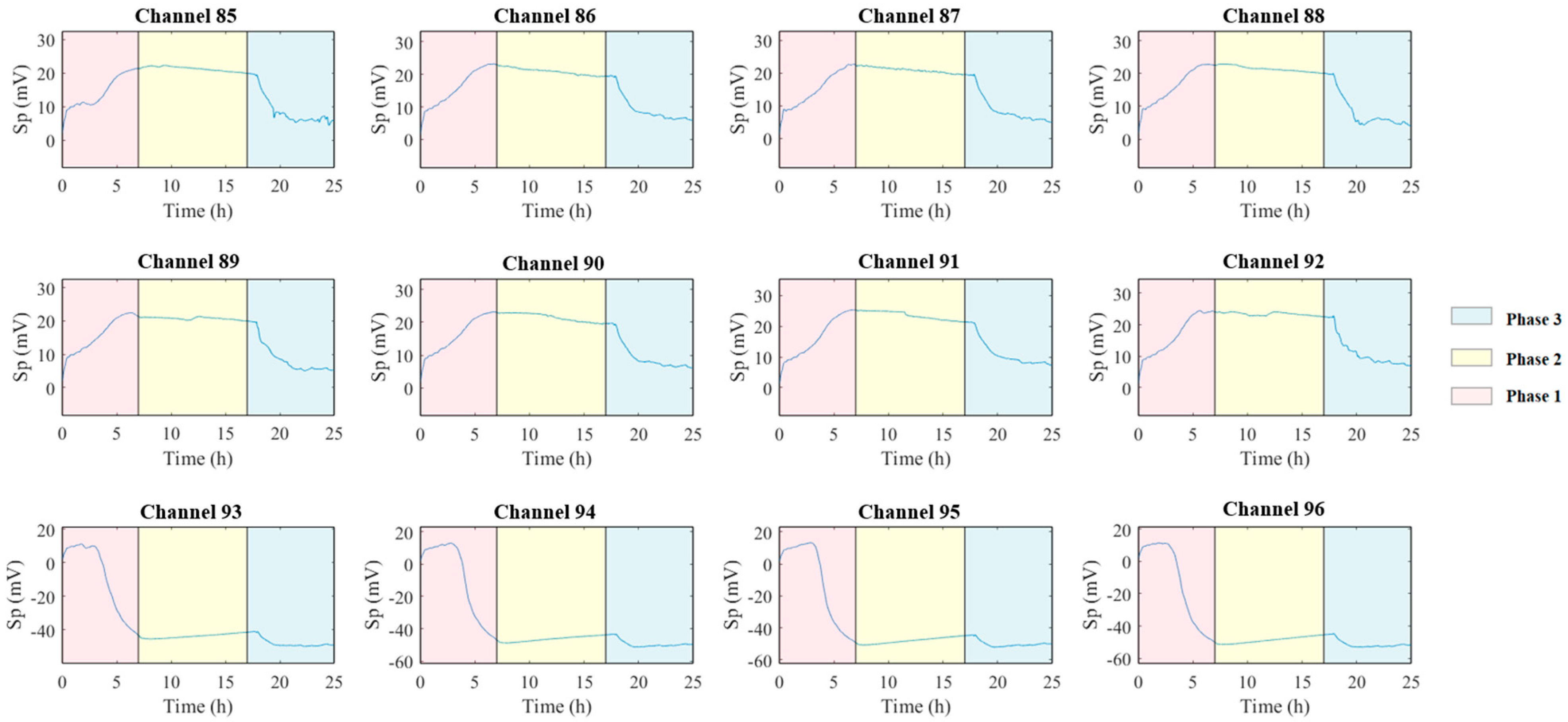
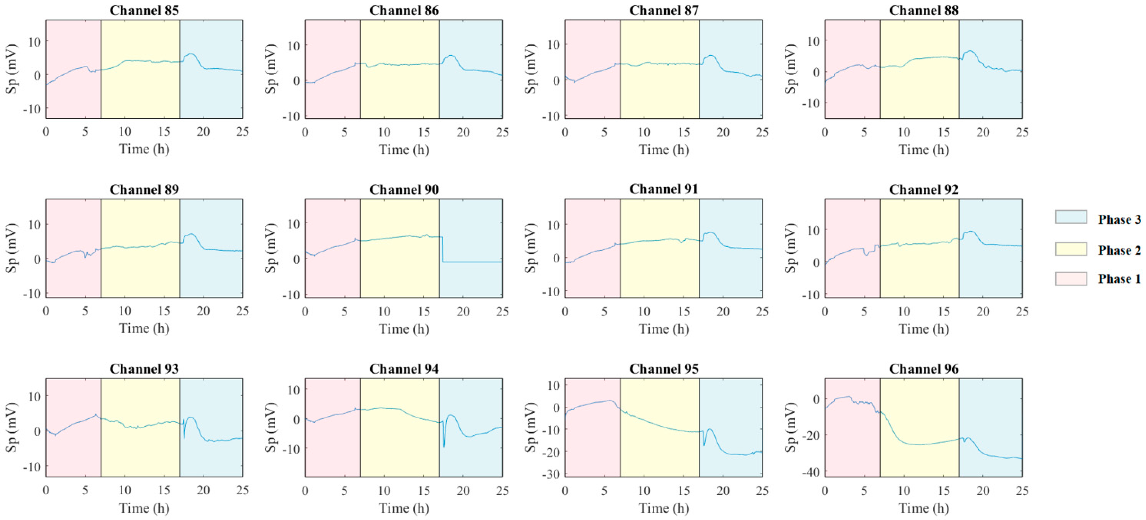
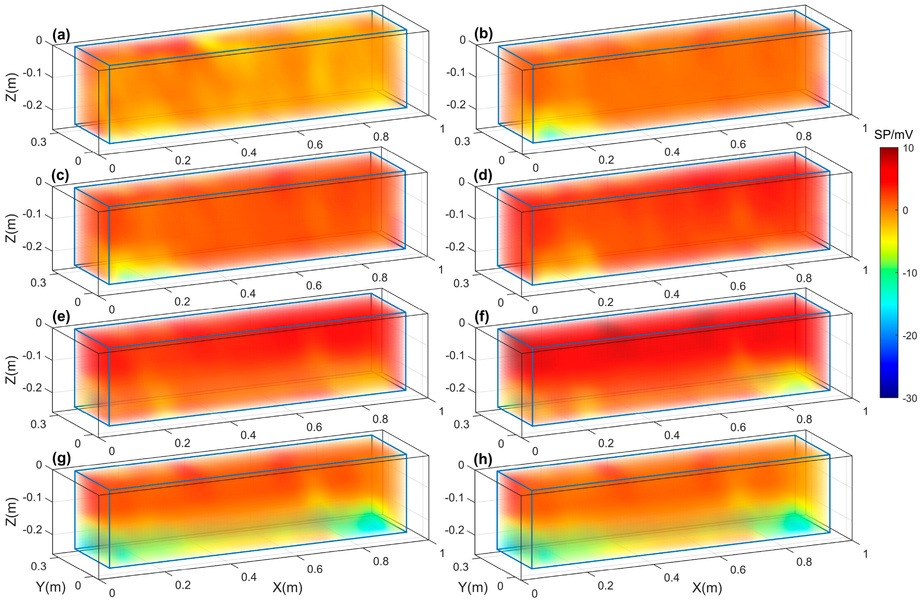
3.1. Laboratory Experimental Simulation

3.1.1. Phase 1: Initial Intrusion (0–7 h)

During the initial phase, saline water intruded from the right chamber into the freshwater-saturated sand in the central chamber. The SP signals and intrusion rates varied significantly depending on the salt concentration. In Experiment (1) (7 g/L salt concentration), the SP values increased gradually from 0 mV to approximately 20 mV, reflecting slow ionic diffusion and the gradual buildup of electrochemical potential. The intrusion rate was 0.034 m/h, which is consistent with the expected slow movement of saline water in low-salinity systems. Notably, all the bottom electrodes (93, 94, 95, and 96) exhibited a sharp drop in SP from 10 mV to −40 mV, suggesting localized ionic imbalances near the saline front. In contrast, Experiment (2) (35 g/L salt concentration) showed a more rapid increase in SP values, from 0 mV to 5 mV, indicating faster ionic diffusion due to the higher salt concentration. The intrusion rate of 0.1 m/h was significantly higher than in Experiment (1), reflecting the enhanced ionic conductivity and steeper electrochemical gradients in the system.

3.1.2. Phase 2: Equilibrium (7–17 h)

During the equilibrium phase, the system stabilized as the saline and freshwater regions reached a balance. In Experiment (1), the SP values stabilized around 20 mV, indicating that the ionic gradients between the saline and freshwater regions had reached equilibrium. This steady state reflects the uniform diffusion of saline water and a stable electrochemical gradient. In Experiment (2), the SP values stabilized at around 5 mV, with a sharper contrast between the saline and freshwater regions. This sharper gradient persisted throughout the equilibrium phase, suggesting that the system remained more dynamic compared to Experiment (1).

3.1.3. Phase 3: Reverse Flow (17–24 h)

In the final phase, the flow direction was reversed to simulate the retreat of the saline front. In Experiment (1), the SP values decreased from 20 mV to around 5 mV, reflecting the gradual retreat of the saline front. The intrusion rate of 0.034 m/h indicates slow ionic diffusion as freshwater replaced saline water. In Experiment (2), the SP values showed a slight increase from 5 mV to 7 mV before returning to 5 mV, indicating more complex ionic dynamics during the flow reversal. The intrusion rate of 0.1 m/h suggests that the system experienced transient fluctuations as the saline and freshwater zones interacted.

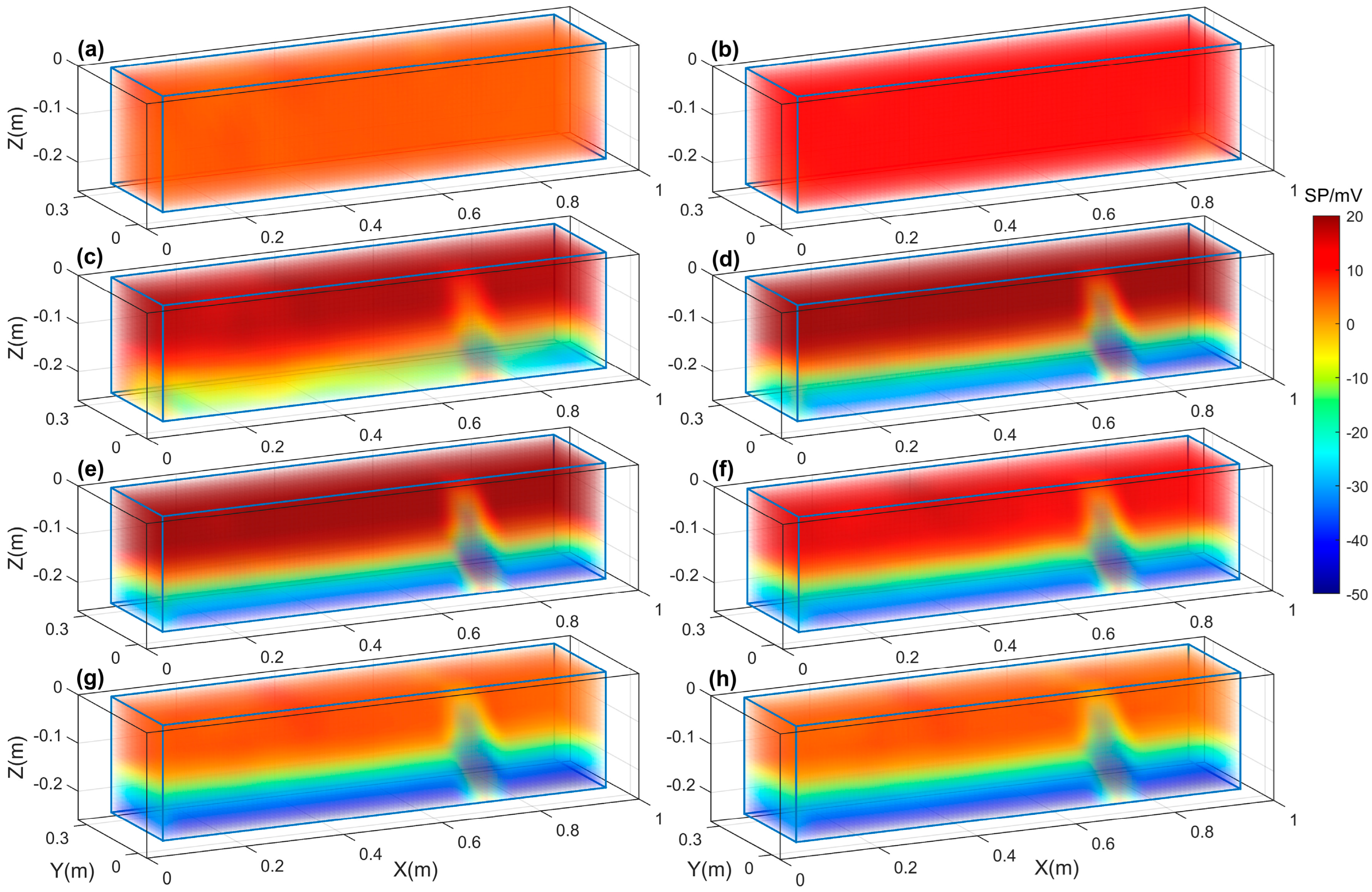
3.2. Numerical Simulation and Model Validation

The primary objective of the numerical simulations was to model the SP anomalies induced by SWI in a controlled laboratory setup. An inclined sheet approximation was used for SP modelling [37], and the Particle Swarm Optimization (PSO) algorithm was employed to optimize the model’s parameters, ensuring the best fit between the measured and simulated SP data. The model aimed to replicate the dynamics of saline intrusion and the electrochemical potential changes under varying salt concentrations of 7 g/L and 35 g/L. The key output of these simulations was the SP signal, which was used to validate the model’s ability to simulate the actual saline front movement and electrochemical gradient development observed in the laboratory experiments. Below are the results of the numerical simulations for each experiment, including the performance of the model and how the RMSE values correspond to the experimental findings.

3.2.1. Experiment (1) (7 g/L Salt Concentration)

In Experiment (1), with a salt concentration of 7 g/L, the model demonstrated an excellent fit with the measured SP data, as Figure 10 shows, achieving a low RMSE of 5.00%. This indicates that the model accurately captured the slow ionic diffusion and gradual buildup of electrochemical potential in the system. The SP values increased steadily over time, from 0 mV to approximately 20 mV, as observed in the laboratory experiments, with a clear and predictable progression from the initial saline intrusion to the equilibrium state.

The intrusion rate of 0.034 m/h was successfully simulated, reflecting the slower ionic transport typical of lower salinity systems. This slow ionic movement allowed the system to build up electrochemical potential over time, which is why the SP signal increased gradually and stabilized at a higher level, aligning well with the experimental observations.

3.2.2. Experiment (2) (35 g/L Salt Concentration)

In Experiment (2), the model’s RMSE increased to 23.45%, reflecting a higher level of complexity in simulating this system, as Figure 11 shows. The ionic diffusion was faster in Experiment (2), resulting in a steeper electrochemical gradient. While the model still captured the 0.1 m/h intrusion rate and the overall trend of the SP values, discrepancies were observed in the sharpness of the ionic gradients and fluctuations during Phase 3, suggesting that the model struggled to replicate the more dynamic ionic transport and its effects on the electrochemical potential.

The rapid ionic diffusion in Experiment (2) created more pronounced electrochemical gradients, which required the model to account for a higher rate of ionic transport. Despite successfully simulating the intrusion rate and overall trend of SP values, the RMSE of 23.45% indicates the model’s difficulty in accurately simulating the sharp ionic gradients and complex dynamics of the system during the flow reversal.

3.3. Sensitivity Analysis Results

The sensitivity analysis was conducted to determine the impact of variations in model parameters (K, x0, z, α, and a) on the simulated SP results for both Experiment (1) and Experiment (2). The analysis was performed at different time steps to assess how changes in these parameters influenced the system’s behavior over time.

3.3.1. Experiment (1) (7 g/L Salt Concentration)

The sensitivity analysis for Experiment (1) showed that the parameters K and z had the most substantial impact on the SP values at various time steps, as is shown in Figure 12. At time 0 h, the sensitivity of K, x0, and α was negligible (all close to 0), while z and a parameters showed low variation. The highest sensitivity for K was recorded at 1 h, with a value of 0.0011, and for z, a value of 0.0034 was recorded at 5 h, reflecting a significant effect of the depth variation on the SP response.

The x0 and α exhibited minimal sensitivity across all time steps, with values generally close to 0. For example, at time 7 h, x0 showed a sensitivity value of −0.4363, while α was virtually constant at 0.0007, showing that these parameters had less influence on the SP behavior in low-salinity systems.

The parameter a demonstrated moderate sensitivity, with the highest value of −1.6647 observed at 5 h. This indicates that changes in the plate length had a noticeable impact on the system, particularly during the intrusion phase as shown in Figure 12.

3.3.2. Experiment (2) (35 g/L Salt Concentration)

In Experiment (2), the sensitivity analysis indicated that the parameter K and z remained the most influential parameters, similar to Experiment (1). However, in this higher salinity system, the parameter x0 showed higher sensitivity, particularly at time 1 h, with a value of 0.2423, reflecting the sharper ionic gradients and more dynamic ionic transport in the system.

The angle α and a parameters exhibited lower sensitivity values compared to K and z parameters, with values close to 0. The sensitivity of α was recorded as 0 for most of the time steps, and a parameter showed its highest value of 1.0738 at time 1 h, suggesting that the half-length of the plate had a relatively minor impact on the system’s behavior in higher salinity systems.

The parameter z demonstrated higher sensitivity in Experiment (2) compared to Experiment (1), particularly at time 20 h, with a value of 0.0673, showing that in the more dynamic environment of higher salinity, the depth of the anomaly center significantly influenced the SP results, as is shown in Figure 13.

4. Discussion

This study demonstrates the SP method’s capability to monitor ionic transport and saline front movement under varying salt concentrations (7 g/L and 35 g/L), contributing to a deeper understanding of SWI dynamics in coastal aquifers. The results align with previous studies and highlight the strengths and limitations of the SP method relative to other techniques.

4.1. Results in the Framework of Previous Studies

In Experiment (1) (7 g/L salt concentration), the gradual increase in SP values from 0 mV to approximately 20 mV, alongside a low intrusion rate (0.034 m/h), aligns with the findings of Graham et al. [28], who observed slow ionic diffusion in low-salinity systems, leading to more gradual electrochemical potential changes. Revil et al. [27] also highlighted that in low-salinity systems, the SP responses are more uniform, which is consistent with our observation that the ionic gradients reached a stable equilibrium at approximately 20 mV. This behavior is further supported by Goswami and Clement [13], who demonstrated that low-salinity systems exhibit predictable and gradual SP changes due to slower ionic transport.

In contrast, Experiment (2) (35 g/L salt concentration) showed a rapid increase in SP values, from 0 mV to 5 mV, and a higher intrusion rate (0.1 m/h). This result mirrors previous studies, such as Leinov and Jackson [16], which have demonstrated that higher salinity systems accelerate ionic transport and generate sharper electrochemical gradients. The faster ionic diffusion and greater ionic conductivity observed in Experiment (2) indicate the influence of salt concentration on both the rate of intrusion and the sharpness of SP gradients in the system. These findings are consistent with Yu et al. [31], who observed similar rapid intrusion rates and sharper gradients in higher salinity systems during laboratory experiments.

The sharp SP anomalies observed near the intrusion source in Experiment (1), particularly at electrodes 93–96, further underscore the role of localized electrochemical processes in influencing SP responses. This finding supports the hypothesis that SP anomalies near intrusion sources are caused by the interaction of saline water with the porous medium, leading to localized charge imbalances (Revil et al. [27]; Graham et al. [28]).

4.2. Interpretation Based on Working Hypotheses

The working hypothesis of this study was that salt concentration would significantly influence both the rate of SWI and the SP response. The results of both experiments confirm this hypothesis. The SP values in Experiment (1) exhibited gradual increases, consistent with the hypothesis that lower salinity systems would show slower ionic diffusion and more stable electrochemical gradients. On the other hand, Experiment (2) demonstrated faster ionic diffusion and more pronounced gradients, supporting the hypothesis that higher salinity systems generate stronger electrochemical potentials and faster ionic transport.

The sensitivity analysis also supports this hypothesis, showing that key parameters like the K and z have a strong impact on the SP values. This is particularly evident in Experiment (1), where K and z showed the highest sensitivity, aligning with the hypothesis that the electrochemical response in low-salinity systems is more influenced by the distribution of ionic concentrations and the depth of the saline front.

4.3. Broader Context and Implications

The findings of this study have broad implications for groundwater management and the monitoring of SWI in coastal aquifers. The ability to use the SP method for real-time monitoring of SWI provides a significant advantage over traditional methods, such as the ERT [41] or ground-penetrating radar (GPR), which often require more complex equipment and may not offer the same level of temporal resolution.

4.3.1. Advantages of the SP Method

• Cost-Effectiveness: The SP method is non-invasive and does not require extensive drilling or sampling, making it a cost-effective option for monitoring SWI. In contrast, methods like chemical sampling (used by Guo et al. [3]) are invasive, time-consuming, and require expensive laboratory analysis. For example, Guo et al. [3] relied on chemical sampling to study contaminant transport in coastal aquifers, which involves collecting and analyzing water samples—a process that is both labor-intensive and costly. The SP method eliminates these drawbacks by providing direct measurements of electrochemical gradients without the need for physical sampling.
• High Sensitivity to Ionic Transport: SP signals are highly sensitive to ionic transport and electrochemical gradients, allowing for real-time detection of saline front movement and localized charge imbalances. This sensitivity is comparable to that of the ERT (used by Folch et al. [26]), but the SP method provides continuous data without the need for complex instrumentation. Folch et al. [26] combined SP with ERT and fiber optic DTS to monitor coastal aquifers, demonstrating that while ERT offers high spatial resolution, SP provides superior temporal resolution for tracking dynamic processes like SWI.
• Real-Time Monitoring: Unlike some geophysical methods that require periodic measurements, the SP method provides continuous, real-time data, making it ideal for dynamic systems like coastal aquifers. This is a significant advantage over image analysis techniques (used by Robinson et al. [22]), which require post-processing and calibration. Robinson et al. [22] used image analysis to study SWI in laboratory setups, but their approach relies on capturing and processing images, which introduces delays and limits real-time monitoring capabilities. The SP method, on the other hand, offers immediate feedback on changes in ionic gradients, making it more suitable for real-time applications.

4.3.2. Limitations of the SP Method

• Complexity in High-Salinity Systems: While the SP method performed well in low-salinity systems, it struggled to accurately capture the sharp fluctuations in SP observed in higher salinity systems (35 g/L). This suggests that the method may be less effective in highly saline environments, where ionic gradients are steeper and more dynamic.
• Dependence on Electrochemical Properties: SP signals are highly dependent on the electrochemical properties of the porous medium and the ionic composition of the fluids [39]. This can make interpretation challenging in heterogeneous aquifers or systems with complex geochemical interactions.

One key implication of the study is the recognition that higher salt concentrations lead to stronger ionic gradients and more dynamic SP behavior, even after the system has reached equilibrium. This has important consequences for coastal aquifer management, as higher salinity systems may be more difficult to mitigate, requiring targeted interventions that account for the more pronounced electrochemical gradients. In contrast, lower salinity systems may allow for slower, more gradual management strategies. Furthermore, the sensitivity analysis indicated that the depth of the saline front and the electric dipole moment are the most sensitive parameters in the SP model, which can inform future modeling efforts. Understanding which parameters most influence SP signals allows for more targeted calibration and refinement of the models used for SWI prediction and monitoring.

4.4. Future Research Directions

Future research should focus on refining the SP method to account for the influence of environmental factors such as temperature fluctuations, which can affect the accuracy of SP measurements. This would improve the robustness of the method, particularly in field applications where environmental conditions may vary. Additionally, extending the use of SP monitoring to heterogeneous aquifer systems would provide more insight into the complexities of SWI in natural settings. Future studies could also explore the combination of SP with other geophysical techniques, such as ERT or GPR, to enhance spatial resolution and depth penetration, especially in deep coastal aquifers.

Another area for future work would be to apply the SP method to study transient behaviors in SWI using different experimental setups as the physical barriers [42], particularly during flow reversals or seasonal fluctuations in coastal aquifers [43]. Investigating the temporal dynamics of SP signals during such phases would provide a better understanding of the long-term evolution of SWI and its potential impact on groundwater resources [44,45].

5. Conclusions

Data collected from laboratory experiments under controlled salt concentrations (7 g/L and 35 g/L) demonstrate distinct SP responses and intrusion rates associated with SWI. In low-salinity systems (7 g/L), SP values increased gradually from 0 mV to 20 mV, with a slow intrusion rate of 0.034 m/h and a model accuracy of RMSE = 5.00%. In contrast, moderate-salinity systems (35 g/L) showed rapid SP changes (0 mV to 5 mV), a faster intrusion rate of 0.1 m/h, and a higher model error (RMSE = 23.45%), reflecting the challenges of modeling complex ionic dynamics in higher salinity environments.

A key finding of this study is the observation of sharp SP anomalies near the intrusion source in low-salinity systems, where SP values dropped significantly from 10 mV to −40 mV at specific electrodes. These localized anomalies highlight the role of charge imbalances in influencing SP responses, providing a potential indicator for the early detection of SWI. Additionally, during flow reversal, low-salinity systems exhibited gradual SP decreases (from 20 mV to 5 mV), while moderate-salinity systems showed transient fluctuations (5 mV to 7 mV). These contrasting behaviors offer new insights into the dynamics of SWI under varying salinity conditions, emphasizing the complexity of ionic transport processes in different environments. The sensitivity analysis also yielded significant results, revealing that parameter K and parameter z are the most influential factors in SP modeling. These findings provide critical insights into the key drivers of SP responses, which can inform and enhance future modeling and monitoring efforts.

Compared to traditional methods such as the ERT and GPR, the SP method demonstrates significant advantages for SWI monitoring. While ERT and GPR are valued for their spatial resolution, they often lack the temporal resolution and ease of deployment offered by SP. The SP method is cost-effective, non-invasive, and user-friendly, making it particularly suitable for real-time monitoring in low-salinity systems. Its ability to detect localized anomalies and provide real-time data positions it as a promising alternative or complementary tool for coastal aquifer management.

References

1. Small, C.; Nicholls, R.J. A global analysis of human settlement in coastal zones. J. Coast. Res. 2003, 19, 584–599. [Google Scholar]
2. Carsel, R.F.; Parrish, R.S. Developing joint probability distributions of soil water retention characteristics. Water Resour. Res. 1988, 24, 755–769. [Google Scholar] [CrossRef]
3. Guo, Q.; Zhao, Y.; Hu, Z.; Li, M. Contamination transport in the coastal unconfined aquifer under the influences of seawater intrusion and inland freshwater recharge- laboratory experiments and numerical simulations. Int. J. Environ. Res. Public Health 2021, 18, 762. [Google Scholar] [CrossRef] [PubMed]
4. Bosserelle, A.L.; Morgan, L.K.; Hughes, M.W. Groundwater Rise and Associated Flooding in Coastal Settlements due to Sea-Level Rise: A Review of Processes and Methods. Earth’s Futur. 2022, 10, e2021EF002580. [Google Scholar] [CrossRef]
5. Cao, X.; Guo, Q.; Liu, W. Research on the Patterns of Seawater Intrusion in Coastal Aquifers Induced by Sea Level Rise Under the Influence of Multiple Factors. Water 2024, 16, 3457. [Google Scholar] [CrossRef]
6. Hauer, M.E.; Hardy, D.; Kulp, S.A.; Mueller, V.; Wrathall, D.J.; Clark, P.U. Assessing population exposure to coastal flooding due to sea level rise. Nat. Commun. 2021, 12, 6900. [Google Scholar] [CrossRef]
7. Werner, A.D.; Bakker, M.; Post, V.E.; Vandenbohede, A.; Lu, C.; Ataie-Ashtiani, B.; Simmons, C.T.; Barry, D.A. Seawater intrusion processes, investigation and management: Recent advances and future challenges. Adv. Water Resour. 2013, 51, 3–26. [Google Scholar] [CrossRef]
8. Zhan, Y.; Murugesan, B.; Guo, Z.; Li, H.; Chen, K.; Babovic, V.; Zheng, C. Managed aquifer recharge in island aquifer under thermal influences on the fresh-saline water interface. J. Hydrol. 2024, 638, 131496. [Google Scholar] [CrossRef]
9. Neumann, B.; Vafeidis, A.T.; Zimmermann, J.; Nicholls, R.J. Future Coastal Population Growth and Exposure to Sea-Level Rise and Coastal Flooding—A Global Assessment. PLoS ONE 2015, 10, e0118571. [Google Scholar] [CrossRef]
10. Dalai, C.; Dhar, A. Impact of beach face slope variation on saltwater intrusion dynamics in unconfined aquifer under tidal boundary condition. Flow Meas. Instrum. 2023, 89, 102298. [Google Scholar] [CrossRef]
11. Henry, H.R. Interfaces between salt water and fresh water in coastal aquifers. US Geol. Surv. Water-Supply Paper 1964, 1613-C, 35–70. [Google Scholar]
12. Voss, C.I.; Souza, W.R. Variable density flow and solute transport simulation of regional aquifers containing a narrow freshwater-saltwater transition zone. Water Resour. Res. 1987, 23, 1851–1866. [Google Scholar] [CrossRef]
13. Goswami, R.R.; Clement, T.P. Laboratory-scale investigation of saltwater intrusion dynamics. Water Resour. Res. 2007, 43, W04418. [Google Scholar] [CrossRef]
14. Chang, S.W.; Clement, T.P. Experimental and numerical investigation of saltwater intrusion dynamics in flux-controlled groundwater systems. Water Resour. Res. 2012, 48, W09527. [Google Scholar] [CrossRef]
15. Vinogradov, J.; Jaafar, M.Z.; Jackson, M.D. Measurement of streaming potential coupling coefficient in sandstones saturated with natural and artificial brines at high salinity. J. Geophys. Res. Solid Earth 2010, 115, B12204. [Google Scholar] [CrossRef]
16. Leinov, E.; Jackson, M.D. Experimental measurements of the SP response to concentration and temperature gradients in sandstones with application to subsurface geophysical monitoring. J. Geophys. Res. Solid Earth 2014, 119, 6855–6876. [Google Scholar] [CrossRef]
17. Ghommem, M.; Qiu, X.; Aidagulov, G.; Abbad, M. Streaming potential measurements for downhole monitoring of reservoir fluid flows: A laboratory study. J. Pet. Sci. Eng. 2018, 161, 38–49. [Google Scholar] [CrossRef]
18. El Hamidi, M.J.; Larabi, A.; Faouzi, M. Numerical modeling of saltwater intrusion in the rmel-oulad ogbane coastal aquifer (Larache, Morocco) in the climate change and sea- level rise context (2040). Water 2021, 13, 2167. [Google Scholar] [CrossRef]
19. Etsias, G.; Hamill, G.A.; Benner, E.M.; Águila, J.F.; McDonnell, M.C.; Flynn, R.; Ahmed, A.A. Optimizing laboratory investigations of saline intrusion by incorporating machine learning techniques. Water 2020, 12, 2996. [Google Scholar] [CrossRef]
20. Sharma, V.; Chakma, S. Experimental Study of Seawater Intrusion in Stratified Layers with Sloping Ocean–Aquifer Boundary. J. Hydrol. Eng. 2024, 29, 04024041. [Google Scholar] [CrossRef]
21. Brunetti, G.F.A.; Maiolo, M.; Fallico, C.; Severino, G. Unraveling the complexities of a highly heterogeneous aquifer under convergent radial flow conditions. Eng. Comput. 2024, 40, 3115–3130. [Google Scholar] [CrossRef]
22. Robinson, G.; Moutari, S.; Ahmed, A.A.; Hamill, G.A. An Advanced Calibration Method for Image Analysis in Laboratory-Scale Seawater Intrusion Problems. Water Resour. Manag. 2018, 32, 3087–3102. [Google Scholar] [CrossRef]
23. Martínez-Pérez, L.; Luquot, L.; Carrera, J.; Marazuela, M.A.; Goyetche, T.; Pool, M.; Palacios, A.; Bellmunt, F.; Ledo, J.; Ferrer, N.; et al. A multidisciplinary approach to characterizing coastal alluvial aquifers to improve understanding of seawater intrusion and submarine groundwater discharge. J. Hydrol. 2022, 607, 127510. [Google Scholar] [CrossRef]
24. Sandberg, S.K.; Slater, L.D.; Versteeg, R. An integrated geophysical investigation of the hydrogeology of an anisotropic unconfined aquifer. J. Hydrol. 2002, 267, 227–243. [Google Scholar] [CrossRef]
25. Morgan, L.K.; Werner, A.D. A national inventory of seawater intrusion vulnerability for Australia. J. Hydrol. Reg. Stud. 2015, 4, 686–698. [Google Scholar] [CrossRef]
26. Folch, A.; del Val, L.; Luquot, L.; Martínez-Pérez, L.; Bellmunt, F.; Le Lay, H.; Rodellas, V.; Ferrer, N.; Palacios, A.; Fernández, S.; et al. Combining fiber optic DTS, cross-hole ERT and time-lapse induction logging to characterize and monitor a coastal aquifer. J. Hydrol. 2020, 588, 125050. [Google Scholar] [CrossRef]
27. Revil, A.; Trolard, F.; Bourrié, G.; Castermant, J.; Jardani, A.; Mendonça, C.A. Ionic contribution to the self-potential signals associated with a redox front. J. Contam. Hydrol. 2009, 109, 27–39. [Google Scholar] [CrossRef]
28. Graham, M.T.; MacAllister, D.J.; Vinogradov, J.; Jackson, M.D.; Butler, A.P. Self-Potential as a Predictor of Seawater Intrusion in Coastal Groundwater Boreholes. Water Resour. Res. 2018, 54, 6055–6071. [Google Scholar] [CrossRef]
29. Crestani, E.; Camporese, M.; Belluco, E.; Bouchedda, A.; Gloaguen, E.; Salandin, P. Large-Scale Physical Modeling of Salt-Water Intrusion. Water 2022, 14, 1183. [Google Scholar] [CrossRef]
30. Stoeckl, L.; Houben, G. How to conduct variable-density sand tank experiments: Practical hints and tips. Hydrogeol. J. 2023, 31, 1353–1370. [Google Scholar] [CrossRef]
31. Yu, X.; Xin, P.; Lu, C. Seawater intrusion and retreat in tidally-affected unconfined aquifers: Laboratory experiments and numerical simulations. Adv. Water Resour. 2019, 132, 103393. [Google Scholar] [CrossRef]
32. Sharma, B.; Bhattacharjya, R.K. Behaviour of contaminant transport in unconfined coastal aquifer: An experimental evaluation. J. Earth Syst. Sci. 2020, 129, 140. [Google Scholar] [CrossRef]
33. Santoso, B.; Hendarmawan; Rosandi, Y. Study of groundwater flow patterns in landslide prone areas using the Self Potential Method. IOP Conf. Ser. Earth Environ. Sci. 2024, 1373, 012012. [Google Scholar] [CrossRef]
34. Kniebusch, M.; Meier, H.E.M.; Radtke, H. Changing Salinity Gradients in the Baltic Sea As a Consequence of Altered Freshwater Budgets. Geophys. Res. Lett. 2019, 46, 9739–9747. [Google Scholar] [CrossRef]
35. Schlesinger, W.H.; Bernhardt, E.S. The Oceans. In Biogeochemistry; Elsevier: Amsterdam, The Netherlands, 2020; pp. 361–429. [Google Scholar]
36. Jougnot, D.; Linde, N.; Haarder, E.B.; Looms, M.C. Monitoring of saline tracer movement with vertically distributed self-potential measurements at the HOBE agricultural test site, Voulund, Denmark. J. Hydrol. 2015, 521, 314–327. [Google Scholar] [CrossRef]
37. Cui, Y.-A.; Zhu, X.-X.; Chen, Z.-X.; Liu, J.-W.; Liu, J.-X. Performance evaluation for intelligent optimization algorithms in self-potential data inversion. J. Cent. South Univ. 2016, 23, 2659–2668. [Google Scholar] [CrossRef]
38. El-Kaliouby, H.M.; Al-Garni, M.A. Inversion of self-potential anomalies caused by 2D inclined sheets using neural networks. J. Geophys. Eng. 2009, 6, 29–34. [Google Scholar] [CrossRef]
39. Ferziger, J.H.; Perić, M.; Street, R.L. Computational Methods for Fluid Dynamics; Springer: Berlin/Heidelberg, Germany; New York, NY, USA, 2002. [Google Scholar]
40. Meyer, R.; Engesgaard, P.; Sonnenborg, T.O. Origin and Dynamics of Saltwater Intrusion in a Regional Aquifer: Combining 3-D Saltwater Modeling with Geophysical and Geochemical Data. Water Resour. Res. 2019, 55, 1792–1813. [Google Scholar] [CrossRef]
41. Costall, A.; Harris, B.; Pigois, J.P. Electrical Resistivity Imaging and the Saline Water Interface in High-Quality Coastal Aquifers. Surv. Geophys. 2018, 39, 753–816. [Google Scholar] [CrossRef]
42. Emara, S.R.; Armanuos, A.M.; Zeidan, B.A.; Gado, T.A. Numerical investigation of mixed physical barriers for saltwater removal in coastal heterogeneous aquifers. Environ. Sci. Pollut. Res. 2024, 31, 4826–4847. [Google Scholar] [CrossRef]
43. Kuan, W.K.; Jin, G.Q.; Xin, P.; Robinson, C.; Gibbes, B.; Li, L. Tidal influence on seawater intrusion in unconfined coastal aquifers. Water Resour. Res. 2012, 48, 2502. [Google Scholar] [CrossRef]
44. Xu, X.; Xiong, G.; Chen, G.; Fu, T.; Yu, H.; Wu, J.; Liu, W.; Su, Q.; Wang, Y.; Liu, S.; et al. Characteristics of coastal aquifer contamination by seawater intrusion and anthropogenic activities in the coastal areas of the Bohai Sea, eastern China. J. Asian Earth Sci. 2021, 217, 104830. [Google Scholar] [CrossRef]
45. Kumar, P.; Tiwari, P.; Biswas, A.; Acharya, T. Geophysical investigation for seawater intrusion in the high-quality coastal aquifers of India: A review. Environ. Sci. Pollut. Res. 2023, 30, 9127–9163. [Google Scholar]
Figure 1. Schematic representation of seawater intrusion laboratory simulation in sandbox model.
Water 17 00941 g001
Figure 2. Real-life sandbox configuration for simulating seawater intrusion.
Water 17 00941 g002
Figure 3. The 192-electrode 3D model for SP data acquisition.
Water 17 00941 g003
Figure 5. The 192-electrode 3D device with the localization of the chosen vertical section from electrode 85 to 96.
Water 17 00941 g005
Figure 6. Vertical section of SP data recorded from electrode 85 to 96 throughout the 24 h duration of Experiment (1).
Water 17 00941 g006
Figure 7. Vertical section of SP data recorded from electrode 85 to 96 throughout the 24 h duration of Experiment (2).
Water 17 00941 g007
Figure 8. Three-dimensional spatial distribution of SP in Experiment (1) during 24 h data recording: (a) 0 h, (b) 2 h, (c) 4 h, (d) 6 h, (e) 12 h, (f) 18 h, (g) 22 h, and (h) 24 h.
Water 17 00941 g008
Figure 9. Three-dimensional spatial distribution of SP in Experiment (2) during 24 h data recording: (a) 0 h, (b) 2 h, (c) 4 h, (d) 6 h, (e) 12 h, (f) 18 h, (g) 22 h, and (h) 24 h.
Water 17 00941 g009
Figure 10. Measured SP versus numerical simulation results for Experiment (1).
Water 17 00941 g010
Figure 11. Measured SP versus numerical simulation results for Experiment (2).
Water 17 00941 g011
Figure 12. The sensitivity over time of the parameters of the 2-D inclined model for Experiment (1).
Water 17 00941 g012
Figure 13. The sensitivity over time of the parameters of the 2-D inclined model for Experiment (2).
Water 17 00941 g013