Abstract
Complex turbulent flow structures are formed within and around box-type artificial reefs (ARs). This study utilizes Particle Image Velocimetry (PIV) and numerical simulation to investigate the flow field within and around ARs of various configurations, such as single- and dual-row arrays. It was found that a small space between reefs causes loading to concentrate on the first reef, while a large space enhances vortex intensity and reduces interference among reefs and promotes vortex development within individual reefs. An optimal space may enlarge the recirculation zone, increase vortex numbers and size, alter the flow distribution, and intensify turbulence, ultimately reshaping the flow characteristics at the reef array. The experimental data show that vortices within ARs attain their maximum strength at an overall reef length to height ratio (Lr/hr) of 3 and reef width to height ratio (Wr/hr) of 0.68. A further increase in Lr/hr weakens the dipole, while an increase in Wr/hr expands the area of high-vorticity and strong turbulence behind the stoss-face openings. These findings provide new insights for the optimum layout of artificial reefs for coastal defense design.
1. Introduction
In recent years, there has been a growing interest in marine ecological environment conservation and protection. Artificial reefs have become widely recognized as an effective coastal structure for marine ecological restoration and protection among coastal nations and regions [1]. Artificial reefs provide habitats and breeding grounds for fish and other marine life by mimicking natural reef environments, thereby increasing fishing ground resources [2,3,4]. Reef structural complexity was found to be correlated with fish abundance and diversity [5]. Studies have shown that artificial reefs can serve as underwater wave attenuation and wave energy harvest structures for coastal protection and marine renewable energy purposes [6,7]. By integrating artificial reefs with submerged breakwaters, an eco-friendly hybrid coastal protection structure can be created, such as box-type artificial reefs (ARs) [8,9]. ARs serve dual functions of coastal protection and fishery enhancement, and their design and layout are critical to improving the marine ecological environment.
Located on the sea bed, ARs are subject to the action of currents, waves, and other types of hydrodynamic environmental forcing. The flow field and force conditions of ARs influence Ars’ hydrodynamic performance [10,11,12]. In the study of reef hydrodynamics, numerical models such as Fluent [13,14] and SPH [15,16] are commonly employed. The flow field induced by ARs is characterized by upwelling in front of the stoss face and wake vortices in the leeside, which promotes water exchange and alters the original flow field [2,14,17]. The exchange between upper and lower water layers can improve the oxygen content and temperature conditions of the lower water layers, while upwelling and wake zones provide abundant food sources and refuge for fish, thereby creating a more suitable habitat for fish and other marine organisms [18]. Therefore, the scale of upwelling and wake vortices is a crucial indicator for the effect of ARs on the flow field. Guo et al. [19] studied the impact of six different structural single ARs on the flow field, established a flow field effect model, and proposed design recommendations for ARs optimized based on flow field volume. Fang et al. [20] conducted a numerical simulation of the impact of double-layer cross-wing reefs on the flow field and found that the side plates of reefs can increase upwelling and obtained the optimal performance. Liu et al. [21] conducted a numerical simulation on frame-type and box-type artificial reefs and found that the internal vortices within the box-type reef are larger than those within the frame-type reef. Furthermore, considerable research has been conducted on star reefs [22], cylindrical reefs [23], mimic reefs [24,25], and semicircular reefs [26]. However, these studies primarily focus on numerical simulations of a single reef’s effect on upwelling and wake vortices.
Based on this previous study of a single reef, scholars have further investigated the flow fields of combined reefs and reef arrays [27,28,29,30]. A previous study by Zheng et al. [13] of single, double, and triple perforated ARs revealed that the turbulence within the reefs was particularly well developed for double reefs, and dipole-type internal vortices were observed under three scenarios. Through numerical simulation, Liu et al. [29] found that the impact of horizontally arranged reefs on the flow field is greater than that of vertically stacked reefs. Mao et al. [30] conducted an optimization study on an artificial reef array with different longitudinal and transverse spacings. It can be observed that the configuration/layout and spacing of reef blocks have a significant impact on the flow field [31,32]. In addition to numerical simulations, physical experiments using Particle Image Velocimetry (PIV) techniques have been carried out to explore the impact of artificial reef shapes, sizes, and configurations on flow velocity, direction, and turbulence intensity [12,33,34,35]. Numerical simulation can predict complex large-scale flow fields around structures under given forcing conditions at the boundaries [36], while PIV technology can provide detailed flow field information. However, the existing research mostly focuses on the flow field characteristics under a single layout or spacing, and it lacks systematic research on different layouts and spacing combinations. These gaps limit the comprehensive understanding of the hydrodynamic performance of artificial reef arrays under pure current.
The flow field effects of ARs are discussed in terms of the magnitude of upwelling and wake vortices near the reef, with little attentions to internal flow characteristics in most of recent studies. When water flows through ARs, small-scale vortices and turbulence are generated within the permeable structure, which directly affect the flow conditions outside the structure. Chaput et al. [37] combined a theoretical analysis and field measurements to demonstrate that micro-scale turbulent vortices in a reef have a significant impact on the cohesion of fish larvae and plankton communities within the reef area. Vortex regions alter water flow structures to create localized areas of high flow velocity. They also disturb sediments, promoting resuspension and redeposition processes, making these regions ideal for fish reproduction, feeding, and spawning [18]. Different structures and layouts of ARs can lead to significant variations in the intensity, direction, and spatial distribution of vortices [38]. Combining PIV experiments and numerical simulations, Jiang [39] observed that both the box-shaped and trapezoidal reefs produced only one vortex within the internal flow fields. Moreover, the internal vortex changed rapidly over time and dissipated upon colliding with the reef structure, with a cycle of approximately 0.2 s. Zheng et al. [13] and Kuang et al. [40] conducted a detailed experimental study of the turbulent structure inside permeable reef-type submerged breakwaters using a PIV test and found a pair of high-vorticity dipolars within the reef. This vortex is induced by the flow jet through the permeable holes on the stoss face and promotes the mixing of water inside and outside the structure. Although there have been a few studies on the internal turbulence and vortex structure of multi-hole box-type artificial reefs from single to combined forms, there is still a lack of research on the changes in internal fluid characteristics under the influence of different reef layouts and overall structural characteristics in combined forms.
In order to fill this gap, based on the previous research [13] on single to triple ARs in one row under pure flow, this paper changes the number of longitudinal reefs, the number of transverse reefs and the spacing of reefs in the combination, and it studies the turbulence and vortex characteristics inside and outside the reefs under different combinations. This study uses numerical simulation to extend the previous study [13] to single- and dual-row arrays with eight reefs and examines the impact of reef spacing on the internal vortex number and strength and turbulence characteristics inside and outside the reefs. Subsequently, PIV experiments are conducted to study the internal hydrodynamic characteristics of the four ARs arranged in a single row, featuring an overall length-to-height ratio (Lr/hr) of 4 and a width-to-height ratio (Wr/hr) of 0.68. The Wr/hr is further increased to 1.36, representing eight ARs in a dual-row arrangement, to further explore the effect of array configuration on the turbulence characteristics inside and near the reef. The aim of the present study is to investigate the impact of the arrangement, spacing, and geometric structures of AR arrays on turbulence, providing a theoretical basis for the future optimization of artificial reef design and deployment.
2. Methods
In the field condition, the flow field around the ARs exhibits a turbulent nature, characterized by a random flow variation in space and time. A combination of PIV tests and numerical simulation was used to explore the turbulent flow induced by AR arrays with various spacings and aspect ratios. This section describes the experiment setup and the establishment and validation of the numerical flume model.
2.1. Experimental Setup
The physical model experiment was conducted in the 6.00 m long, 0.45 m wide, and 0.55 m high flume in the Hydrodynamic Laboratory of Shanghai Ocean University, China (cf. Figure 1). Polyvinyl chloride micro-powders (PVC-6500, TSI Incorporated, Shoreview, MN, USA) were used as tracer particles. And the PIV technique developed by TSI Incorporated, USA, was used to measure the flow field. The particles in the flow were illuminated by a laser light, and the positions of the particles on the plane were captured by a charge-coupled device (CCD) camera (TSI Incorporated, USA). Using the synchronizer, the computer could display the images captured by the CCD camera in real time, thereby continuously recording the time series of the instantaneous particle positions near ARs. Based on the PIV algorithm, the velocity vector at these positions, and, therefore, the flow field, including the turbulent component, was derived. The schematic diagram of the PIV system is shown in Figure 1.
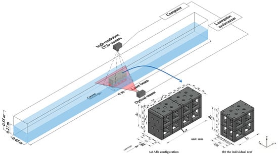
Figure 1.
Schematic diagram of PIV system and flume setup and AR model. (a) ARs’ configuration; (b) the individual reef.
The ARs in this experiment mimic the prototype deployed at the Beidaihe coastal site, China. Based on the water depth at the Beidaihe site [41,42] and the flume size, the experiment was designed with a geometric scaling of 1:12.5. An individual reef was lr = 0.224 m length, wr = 0.152 m wide, and hr = 0.224 m high. The reef stoss face and crest contained four circular permeable holes with a diameter of 0.024 m, as detailed in Figure 1b. To facilitate PIV measurements, the reef was made of transparent organic glass material with a light transmittance of 96%.
In this experiment, the water depth was 0.27 m, and the inlet discharge was set to 40 m3/h. Correspondingly, the average inlet flow velocity was v0 = 0.091 m/s, with the ARs fully submerged. During the experiment, the inlet flow velocity, water depth, and the location of the first reef are constant.
To observe the three-dimensional turbulent flow field around ARs, the PIV system mainly measured the vertical section (Y = 0.03 m), the near-bottom horizontal section (Z = 0.068 m), and the near-surface horizontal section (Z = 0.156 m). The vertical section passed through the first row of circular holes on the crest, while the near-surface and near-bottom horizontal sections passed through the upper and lower rows of circular holes on the reefs’ stoss face. At each section, 500 instantaneous flow fields were continuously captured at a sampling frequency of 4.83 Hz. The instantaneous flow field data were then averaged to obtain the time-averaged flow field parameters.
2.2. Numerical Model Setup
In order to further explore the response of the hydrodynamics near the ARs to current action, a 3D numerical flume model was constructed, and ANSYS FLUENT 17.0 software was employed to compute the flow field due to current–structure interactions. The flow was assumed to be incompressible, steady, and viscous. The governing equations consist of the continuity equation and the Reynolds Average Navier–Stokes equation (RANS) for viscous incompressible flow. The finite volume method (FVM) was employed for spatial discretization, and the SIMPLE algorithm was used for pressure–velocity coupling. The governing equations were discretized using a second-order upwind scheme to enhance the numerical accuracy. An eddy viscosity and mixing-length model and a one-equation and two-equation turbulence model have been developed to parameterize the contribution of the turbulence flow to the Reynolds Average Navier–Stokes equation [43]. Here, the two-equation k-ε turbulence model was implemented to represent turbulent flow in the RANS model.
For incompressible flow, the Reynolds-averaged Navier–Stokes equation and continuity equation are given by
where i, j = 1, 2, 3, corresponding to the Cartesian coordinate system directions x, y, z, respectively; xi and xj represent the coordinate components; and are the time-averaged velocity component in each direction; t represents time, s; ρ is the fluid density, kg/m3; is time mean pressure; fi is the mass force component; and ν is the kinematic viscosity of the fluid. The Reynolds stress term represents the momentum flux between turbulent and mean flow. A new turbulent model for the Reynolds stress term must be introduced to close the equation.
Based on the Boussinesq eddy viscosity assumption, the relationship between the Reynolds stress and velocity gradient is established by introducing turbulent viscosity (μt).
where μt represents the turbulent viscosity, also known as the eddy viscosity coefficient; δij = 0 (i ≠ j) or 1 (i = j); and k is the turbulent kinetic energy given by
where , , and represent the turbulent component of velocity in the x, y, and z directions, respectively.
The standard two-equation k-ε turbulence model solves for the eddy viscosity coefficient (μt) through the turbulent kinetic energy (k) and the turbulent dissipation rate (ε) equation [44] in (5) and (6):
where μ represents the dynamic viscosity; Dk is the dissipation term of turbulent kinetic energy k; Gb represents the turbulent kinetic energy production term due to buoyancy effects; and Gk is the production term of turbulent kinetic energy k induced by turbulent stress or velocity gradient given by
where σk, σε, C1ε, C2ε, C3ε, and Cμ are the empirical constants or modified variables described in Launder and Spalding [44].
The standard two-equation k-ε turbulence model often does not perform well in adverse pressure gradients and separations [45]. Considering the intricate three-dimensional flow around the reef, the complexity of the ARs’ structure and internal flow, and the balance between computational accuracy and efficiency, the modified k-ε model by Shih et al. [46], which incorporates swirl correction and a refined eddy viscosity coefficient, is adopted for the present study. Cμ in Equation (9) is no longer a constant but a function of k, ε, and the rotation strain rate U*.
where A0, and As are empirical constants.
The dissipation rate (ε) equation is derived from the transport equation of the mean-square vorticity fluctuation. The ε equation includes an additional source term , where ν is the kinematic viscosity, to better describe the transport of turbulent energy spectra.
The structure and dimensions of ARs in the numerical model are same as in the physical test. The length of the computational domain was set as 5lr (lr is the length of an AR block) in front and 10lr behind the reef array. The velocity boundary condition was employed at the inlet. Zero mean static pressure was implemented as the pressure boundary condition at the outlet. A no-slip boundary condition was applied at the reef structure and flume walls. The shear stress at the top boundary of the computational domain was set to zero, simulating a moving wall at the flow velocity.
The mesh was generated using tetrahedral unstructured grids. There was a very thin boundary layer in the near-wall region of the ARs. The first layer of the boundary mesh was set to a thickness of 0.5 mm, with a growth rate of 1.1. Local refinement was performed on the stoss face, crest, and inner walls of the permeable circular holes. The grid independence study was performed by refining the grid until variations in key flow parameters, i.e., velocity magnitude, vortex performance, and vorticity, were within 3%. The final grid resolution was determined based on this criterion, with the total number of grids being 292.01 × 10⁴. The detailed grid is shown in Figure 2.
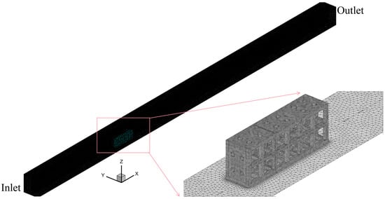
Figure 2.
Schematic diagrams of the computational domain and grid.
The non-dimensional Courant number (CFL) was maintained below 0.5 to ensure numerical stability. A time step of Δt = 10−3 s was selected based on preliminary testing to balance computational efficiency and accuracy. Convergence was monitored through residuals, with the continuity equation and momentum components converging to 10−5 and turbulence kinetic energy converging to 10−6. In addition, integral quantities such as drag coefficients and turbulence intensity were tracked to confirm steady-state behavior.
The standard k-ε model was selected for its robustness and efficiency in predicting flow characteristics around bluff bodies, such as artificial reefs. However, this model’s reliance on wall functions may introduce errors in near-wall regions, especially for strong recirculating flows. To mitigate this, the standard wall function approach, with y+ values maintained within the recommended range (30 < y+ < 200), was used to ensure valid log-law behavior.
2.3. Model Validation
The present numerical model was previously validated by Zheng et al. [13] and Kuang et al. [14] against PIV measurements of a single reef for its accuracy in simulating physical experiments for reef systems. To account for the increased complexity of turbulence in the vicinity of multiple ARs, the model was re-validated by PIV results of a single-row three-AR experiment. Velocity profiles (vxz) (Y = 0.03 m) from the PIV and numerical model near the ARs were extracted from the vertical sections at the dashed lines in Figure 3. Figure 3a,b show the PIV and numerical model results at vertical S1-S1, S2-S2, and S3-S3 located at the leeside of the first, second, and third reef blocks, respectively, whereas Figure 4 shows the comparison of modeled and PIV measurements of longitudinal velocities.
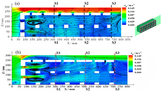
Figure 3.
Time-averaged vertical flow field for the single-row three-reef array with vertical lines S1-S1, S2-S2, and S3-S3 located at the leeside of the first, second, and third reef blocks, respectively. (a) PIV experiment; (b) numerical model. White areas indicate the presence of a reef array.
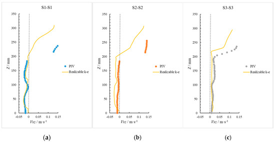
Figure 4.
Comparison of the PIV and numerical model results of the velocity at vertical lines (a) S1-S1, (b) S2-S2, (c) S3-S3 for the single-row three-reef array.
Figure 4 indicates that the numerical model compares well with the experimental data in the external regions, except for the area above the crest, where experimental flow velocities are higher than the numerical results, with a maximum error of 0.11 m/s. The discrepancy may stem from a limited grid resolution and wall treatment of zero shear stress at the crest in the model, as well as PIV measurement errors due to optical constraints and particle shadowing, particularly in the vicinity of the structure and walls. The model predicted a stronger jet flow through the hole at the stoss face and, therefore, weaker flow above the crest according to mass conservation. Additionally, the transient flow conditions in the experimental data versus the average basis of the numerical model could also contribute to the discrepancy. Despite the mismatch above the crest, both model and PIV measurements show similar flow direction and distribution patterns, in particular in the vortex structures and most flow field characteristics within the ARs. Although the numerical model did not capture the flow separation within the third AR, it well resolved the observed distinct wake on the backside of the ARs.
2.4. Test Conditions
The relationship between the turbulent characteristics in the vicinity of the reef groups and the spacing among the ARs in a single row was examined in the numerical model. The non-dimensional parameter d/lr was introduced, where d was the longitudinal distance between adjacent ARs in the flow direction, and lr was the length of an AR block. The inflow velocity was set to 0.09 m/s. And the relative submergence R/h above the AR was 0.17, where R was the reef submergence and h was the water depth. The simulation conditions are shown in Table 1.

Table 1.
Model setup and the AR spacing relative to AR length d/lr. and relative AR submergence R/h.
In addition to the impact of spacing between ARs, the PIV physical model experiments were used to explore the effects of size changes in the overall structure of ARs on their surrounding flow field. Based on the experiment with three ARs with no spacing in between in a single row, the number of reefs was increased in the length and width directions, respectively, to change the overall AR array size. The overall dimensions of the AR array were defined by Lr for the total length, Wr for the total width, and hr for the total height. And the aspect ratios were expressed as Lr/hr for the length-to-height ratio and Wr/hr for the width-to-height ratio. The experiment setup is shown in Table 2. Among them, Condition 5 indicates the 3 ARs in a row condition, and the experimental results were adopted from Zheng et al. [13] in 2022.
Table 2.
Experimental conditions of ARs’ array layout and overall dimension.
3. Results and Discussion
3.1. Impact of AR Spacing on Flow Characteristics
3.1.1. Vertical Flow Fields
Figure 5a–d show the modeled vertical flow fields induced by three ARs arranged longitudinally with spacing ratios d/lr = 0, 0.5, 1.0, 3.0. When the spacing ratio is zero (d/lr = 0), that is, the ARs are located next to each other, the three ARs can be treated as an integral structure present in the flow field. Therefore, the flow field characteristics in the vicinity of the ARs are largely determined by the first reef block in the direction of incoming flow. At x = −0.2 m, the streamlines experience a significant change. The main free stream flow is lifted up at the reef stoss face, forming the upwelling flow. Near the bottom of the reef (0 m < z < 0.1 m), the flow moves downward along the first reef stoss face due to the blocking effect of the structure and forms the small vortex structure near the bottom. Moreover, a part of the water flow into the ARs through the opening holes is distributed on the first reef’s stoss face. And a vortex structure can be found near the stoss face of the first AR, especially to the rear of its permeable holes.
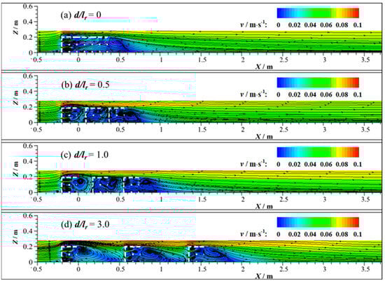
Figure 5.
Model results of vertical flow fields for the three ARs in a single row with AR spacings: (a) d/lr = 0; (b) d/lr = 0.5; (c) d/lr = 1.0; (d) d/lr = 3.0.
As the AR spacing increases, the vertical flow field characteristics inside and outside the ARs change significantly. For d/lr > 0, the stoss face of each AR is in direct contact with the fluid as the spacing ratio gradually increases. The pressure difference behind each reef results in a wake current of various strengths. With the increase in d/lr, the extent of the wake current behind the ARs increases. The backflow formed behind the first two ARs is weakened by the ARs behind. However, the weakening effect becomes smaller as the distance between ARs increases, to a certain value when the backflow can be fully developed. The spacing of ARs is a key factor for the flow field, which in turn affects the performance of the ARs. Moreover, vortex structures with various scales and intensities are formed within the ARs with the change in the spacing ratio and so make the complex turbulence structure. Notably, within each reef, there is very little variation in the morphology and number of vortex structures. This suggests that the internal flow of each AR block, especially the internal vortex structure, are not altered much; nevertheless, the AR spacing changes the whole system flow field considerably. The relatively stable internal flow field within each AR is critical to the understanding and design of ARs, as well as in the analysis of the associated turbulence flow.
In addition, with an increasing AR spacing ratio, the degree of mutual interference between adjacent blocks decreases, and the vortices inside the AR structure can be more developed. So, when d/lr > 0.5, the number, size, and intensity of the vortices formed inside the individual AR also show a gradual increase with the increase in d/lr.
3.1.2. Vorticity and Turbulent Intensity
As mentioned above, the turbulent flow is changed by the AR array configuration, and various scales of vortex structures appear in the flow field. Vortices can enhance the water exchange and mixing and energy dissipation, which is an important design consideration of ARs. The size and distribution of vortices directly reflects the rotation of fluids at the macroscopic scale. The vorticity components in the vertical and horizontal planes are represented by Ωy and Ωz, respectively, and are calculated based on the corresponding flow field data.
where vx is the longitudinal velocity, vy is the lateral velocity, vz is the vertical velocity, and Ωy and Ωz represent the strength of the vortex rotation along the lateral and longitudinal directions, respectively.
In order to analyze the vortex formation and vorticity distribution for ARs with different spacing ratios, Figure 6 shows the y-component of vorticity (Ωy) associated with the vertical flow field. As shown in Figure 6, two pairs of high-vorticity dipoles (|Ωy| ≥ 1.5 s−1) are observed behind the opening holes on the stoss face of the first AR for all test conditions. Each pair consists of two vortices with a similar intensity but opposite rotation direction, which are symmetrical in the vertical direction [47]. When the flow passes through the opening hole on the stoss face, the formation of vortices occurs due to changes in velocity and the curvature of the flow streamlines.
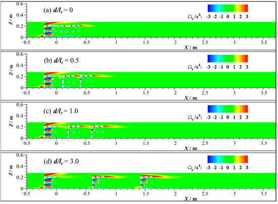
Figure 6.
Vertical distribution of vorticity predicted for three ARs in a single row with AR spacing: (a) d/lr = 0; (b) d/lr = 0.5; (c) d/lr = 1.0; (d) d/lr = 3.0.
For d/lr < 0.5, high-vorticity dipoles are observed at the first reef. For d/lr = 1.0, the vorticity dipoles behind the stoss face of the last AR become more evident, while there is still little vorticity formation inside the middle AR. When d/lr increases to 3.0, vorticity dipoles are found in each AR. And due to the influence of the front and rear ARs, the flow at the second AR is restricted, so that turbulence development is limited. The strength of the vorticity dipole formed in the second reef is weaker than that of the other reefs; so is the turbulence intensity. This finding indicates that the spacing of adjacent reefs is critical to the flow field characteristics within the AR system. As d/lr increases, the backflow region expands. Additionally, the quantity and scale of internal vortices increases, and the flow field pattern in and around the individual reefs is modified and turbulence is intensified, which in turn influences the overall flow field of the entire AR system. Moreover, each reef in the system forms nearly independent vortex structures in the flow field, which are essential for maximizing the impact of ARs on the flow field.
In addition, turbulence intensity represents the degree of fluctuation of flow velocity or the irregularity of fluid movement [48]. Turbulence intensity in this study is defined as the ratio of the standard deviation of fluctuating velocity to the mean velocity. To determine the turbulence intensity, the time-averaged velocities in each direction and their corresponding turbulence intensities are defined as follows,
where vi represents the instantaneous velocity in the i-th direction (i = x, y, z); N is the total number of instantaneous velocity fields captured by the PIV system during the entire measurement period; and δi is the total standard deviation of the velocity component in the i-th direction, representing the turbulence intensity in different directions. The total turbulence intensity obtained in a two-dimensional plane is calculated using the following formula,
where Ixy and Ixz represent the total turbulence intensity in the horizontal plane and the vertical plane, respectively.
Figure 7 shows the vertical distribution of turbulence intensity induced by ARs with different spacing ratios under the same inflow conditions. Due to the stable inflow conditions, a low-turbulence area appears in front of the first reef at all spacing ratios. The high-turbulence area is mainly located at the opening holes on the stoss face of the first reef, which is also approximately the location of the high-vorticity dipoles. This phenomenon can be explained by the fact that when the flow encounters the solid surface, the flow tunnels through the hole where velocity is highest. In addition, it also shows that the turbulent intensity is higher in the region with high-vorticity dipoles. With the increase in d/lr, the turbulence intensity between adjacent reefs increases. Between adjacent ARs, a high-turbulence area appears in front of the second reef’s stoss face. As the ratio d/lr grows, the high-turbulence region stretches from the stoss face of the second reef to the rear of the first reef. When d/lr = 3.0, the range of the high-turbulence region attains the maximum.
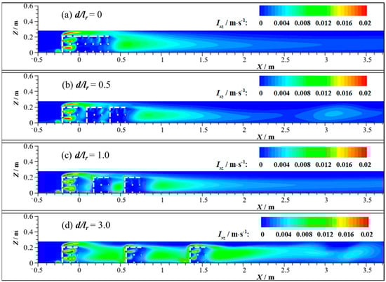
Figure 7.
Predicted turbulent intensity distribution in vertical section at Y = 0.03 m induced by the three ARs in a single row with relative AR spacings: (a) d/lr = 0; (b) d/lr = 0.5; (c) d/lr = 1.0; (d) d/lr = 3.0.
The turbulence intensity above the reefs is also large with the fluid passing through the ARs. The high-turbulence area occurs at the crest of the first AR. This could be attributed to faster flow and the large disturbance exerted on the fluid by the reef crest. The flow velocity fluctuates significantly, and the turbulence intensity is enhanced. When d/lr = 1.0, the turbulence intensity on the crest of the latter two ARs increases. With the increase in d/lr to 3.0, the flow between ARs is relatively fully developed, and high turbulence intensity occurs on the crest of each reef.
3.2. Impact of Dimensions of AR Array on Flow Characteristics
The previous section mainly focused on the effect of AR spacing, but the impact of the geometric structure of ARs on the variation in turbulent characteristics is also important to the performance of ARs. The scope of the previous study [13] is extended here. PIV experiments with four ARs in a single row were conducted to assess the influence of the total length of ARs (increase in the Lr/hr). Furthermore, the influence of the total width of ARs on the flow field was investigated through PIV experiments of eight dual-row reefs.
3.2.1. Effect of AR Array Length on Flow Characteristics
Figure 8 illustrates the time-averaged flow field of single-row four-body ARs arranged longitudinally for an Lr/hr to 4. The vector lines in the figure represent the streamlines, with the color contour lines reflecting the magnitude of the flow velocity, and the green transparent area depicts the vertical section of ARs. In this section, the single-row one-to-three-reef results in Figure 3a from Zheng et al. [13] are used for comparison.
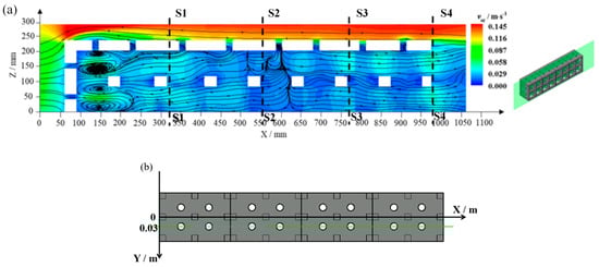
Figure 8.
(a) (Left) Predicted time-averaged vertical flow fields for the four ARs in a single row with the average inlet flow velocity v0 = 0.091 m/s. (a) (Right) Diagram of profiles captured (green transparent area exhibited on the right). (b) The top view of the location of the vertical section (z-x) shown in the plot on the left.
Compared to Figure 3a, Figure 8 shows that the upwelling flow also appears in front of the ARs in the four-reef configuration, with the maximum upwelling flow velocity occurring at a position similar to that in the three-reef configuration. However, the maximum upwelling flow velocity is slightly reduced to 0.145 m/s, which is 1.8 times the mainstream velocity (approximately 0.08 m/s). Furthermore, the four-reef arrangement extends the entire length of the AR system, resulting in an elongation of the high-velocity zone above the ARs and the low-velocity recirculation zone within the ARs.
As shown in the vertical flow field within the ARs, two quasi-symmetrical high-velocity zones form behind the opening holes on the stoss face due to the jet flow entering the stoss face and separating from the rest of the internal water, leading to the formation of counter-rotating vortices. This phenomenon is consistent with the counter-rotating vortex pair (CVP) observed by Gutmark et al. [49] in multi-hole jet cross-flows. The extended AR system moves the third reef block from the end to the middle of the system, reducing the wake flow influence and turbulence intensity within the ARs. Inside the third reef block, the diverging flow is evident, with water splitting towards the stoss face and leeside. Moreover, while the first two reef blocks exhibit flow opposite to the mainstream, the last two reef blocks show flow in the same direction as the mainstream. The extension of the AR system by adding the fourth reef block also significantly alters the distribution of vertical flow within the ARs. After the mainstream crosses the ARs, a backflow region is formed behind the whole AR system. The previous study [13] has shown that under single-row arrangements, from one to three blocks, there is a large clockwise vortex in the backflow region. The internal flow pattern is dominated by the backflow entering from the leeside. However, as the entire length of the AR system extends, the distance of the wake vortex behind the ARs from the leeside increases. And the internal flow pattern changes to become dominated by the inflow through the opening holes on the first stoss face and the rear side of the crest of the AR array. In addition, the energy dissipation to the mainstream caused by the reef crest increases, resulting in a decrease in the flow velocity above the crest.
To better understand the impact of the increased length of the AR array, the vertical vorticity distribution and turbulent intensity distribution was also investigated. Figure 9a illustrates the vertical vorticity (Ωy) distribution for the four-reef ARs, with the arrows indicating the vertical flow velocity direction. Figure 9b illustrates the distribution of total turbulence intensity on the vertical profile for the ARs.
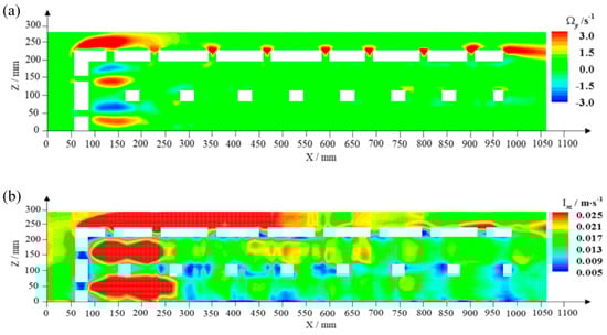
Figure 9.
Vertical distribution of (a) vorticity and (b) turbulent intensity along a vertical section for four-reef ARs in a single row.
It is evident from Figure 9a that the presence of the ARs results in high-vorticity (|Ωy| ≥ 1.5 s−1) areas both inside and outside the ARs near the holes. Externally, when the strong upwelling flow in front of the first reef block passes its sharp upper left corner, shown in Figure 8a, the vorticity is amplified and spreads along the reef crest. The pressure gradient near the ARs creates a siphon-like effect, driving flow mixing, and the crest’s opening holes are vortex hotspots due an interaction with the strong flow above the crest in Figure 8a. High vorticity occurs after strong flow interaction with the sharp upper right corner of the last reef block. Internally, behind the opening holes on the first reef stoss face, two pairs of dipoles with high vorticity are formed, each with a clockwise lower vortex and a counterclockwise upper vortex. The extension of the total length of the AR system by adding the fourth reef block slightly reduces the internal high-vorticity intensity but hardly changes its position, confirming that the internal turbulent pattern is primarily influenced by the stoss face opening rather than the total length of the AR system.
Figure 9b shows a similar turbulence intensity distribution near ARs as the previous study for three reefs in a row [13]. High-turbulence areas appear above the ARs’ crest and inside the first block, corresponding to the high-vorticity zone. Unlike the three reefs array, the increase in the total length of the AR array reduces the turbulent intensity at the leeside of the ARs. And the turbulent intensity above the crest exhibits a decreased extent but increased strength. The turbulence intensity above the crest of the third block is significantly reduced. This decrease in turbulence intensity outside the ARs is likely due to the addition of the fourth reef block, which increases energy dissipation, reduces mainstream velocity, and decreases the pressure difference, thereby weakening the flow separation around the structure in these areas.
3.2.2. Effect of Reef Array Width on Flow
The length-to-width aspect ratios of the box-type artificial reefs (ARs) significantly influence their flow dynamics [50]. This section examines a dual-row eight-reef array to explore the effect of reef array width on water exchange and flow dynamics and compare it with a single-row four-reef array. Figure 10 shows the flow field for the dual-row eight-reef array.
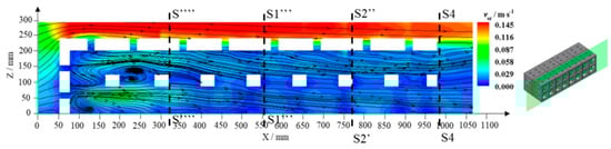
Figure 10.
(Left) Time-averaged flow field of the dual-row eight-reef array in the vertical section indicated by the green color across the reef array (Right). The arrows on the graph indicate the direction of the streamline.
Similar to other reef configurations, upwelling occurs in front of the ARs’ stoss face. With an increased total width-to-height ratio (Wr/hr) of 1.36 and more overall flow blockage, more fluid rises from the bottom to above the crest, and the stoss face area doubles, broadening the upwelling’s lateral extent. The wider reef array enhances water retention, minimizes side overflow, and, therefore, creates a higher-speed upwelling above the crest, reaching larger maximum velocities above the reef array. The expanded array in the spanwise direction provides more space for internal flow development and more streamlined flow. The internal flow behind the vortex structure aligns with the mainstream and sustains lower velocities. The leeside wake vortex formed is further away from the reef than that in single-row configurations.
The width, however, has a limited effect on the vertical flow pattern. Hence, the rest of the discussion will focus on horizontal flow characteristics. Figure 11 shows the horizontal flow fields in the near-bottom and near-crest vertical layers for single-row four-reef and dual-row eight-reef arrays. It shows significant flow separation and recirculation zones downstream of the stoss face, with a symmetrical vortex distribution across the horizontal plane. The increased reef block number results in distinct elliptical high-velocity zones behind the upper and lower stoss face opening holes and a weakened internal vortex due to internal vortex interactions. Additionally, the internal flow pathways become more streamlined with more blocks, with reduced vortex formation.
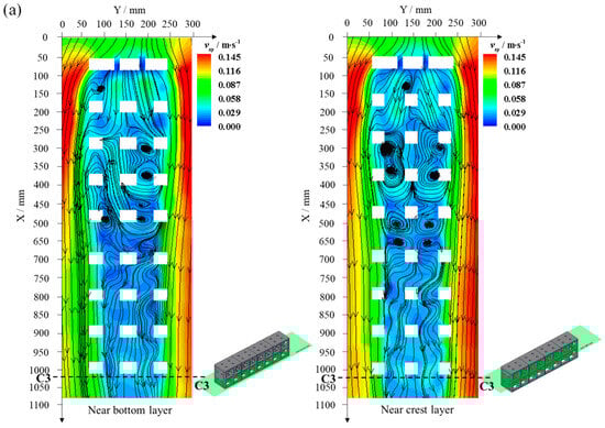
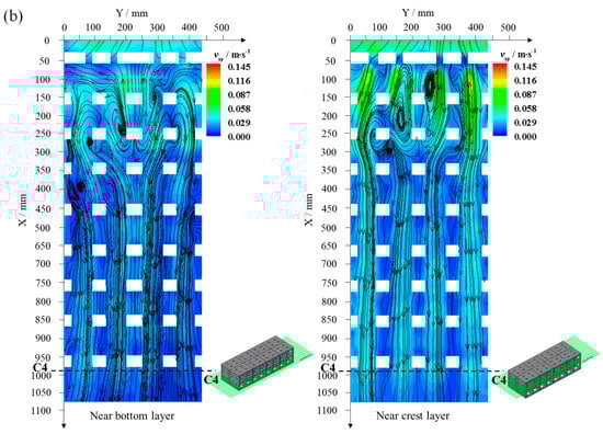
Figure 11.
Time-averaged horizontal flow fields in the near-bottom and near-crest vertical layers for (a) single-row four-reef array and (b) dual-row eight-reef array. The layers were indicated by the green color across the reef array. The arrows on the graph indicate the direction of the streamline.
Figure 12a,b display the horizontal distribution of vorticity (Ωz) in the near-bottom and near-crest vertical layers for a single-row four-reef array and dual-row eight-reef array. The maximum values for each vortex dipole are indicated in Figure 12. It is observable that the vorticity pattern in the near-bed and near-surface layers is similar, with stronger vorticity near the surface. The blockage effect of ARs deflects the flow to move upwards along the stoss face. Additionally, the opening holes on the crest facilitate the exchange of water between the interior and the surroundings, resulting in stronger vorticity in the surface layer than the bottom layer. The vortex number and strength for the dual-row array are markedly less than those for the single-row array. And the high vorticity is concentrated in the first reef block. Four pairs of strong dipolar vortices are observed near the surface with a maximum vorticity of 5.000 s−1. Near the bottom, each pair of dipolar vortices consists of one strong and one weak vortex with opposite directions, with a maximum vorticity of 2.000 s−1, which is less half of that near the surface. In the single-row array, the intensity of vortices near the bottom and the surface is comparable. These results indicate that the dual-row array significantly influences the vertical distribution of flow in the vicinity of the ARs. The upper layer flow is damped more than the lower layer under the dual-row arrangement.
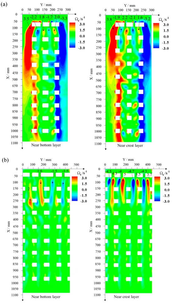
Figure 12.
Horizontal distribution of vorticity, Ωz, in the near–bottom and near–crest vertical layers. (a) Single-row four-reef array; (b) dual-row eight-reef array.
To quantify the impact of a single-row and dual-row configuration and dimension on the vortices within ARs, the single-row three-reef array is used as the control case. The area of the high-vorticity (Ωz) zone in the horizontal plane within the structure and the average vorticity (Ωz) in that area were extracted for both scenarios and listed in Table 3.
Table 3.
The area and average vorticity of internal high-vorticity region (|Ωz| > 1.5 s−1) for ARs with different total width-to-height aspect ratios.
As shown in Table 3, the area occupied by the high-vorticity zone (∣Ωz∣ > 1.5 s−1) within the artificial reef varies significantly between different configurations. The results indicate that Condition 3 (Lr/hr = 5, Wr/hr = 1.36, eight blocks) exhibits the largest high-vorticity zone, covering approximately 2.799 × 10⁻³ m2, which is 41.5% larger than Condition 1 (Lr/hr = 3, Wr/hr = 0.68, three blocks). Conversely, Condition 2 (Lr/hr = 4, Wr/hr = 0.68, four blocks) results in the smallest high-vorticity region, covering only 0.831 × 10⁻³ m2, a 58% reduction compared to Condition 1. The variations suggest that the total reef width-to-height ratio (Wr/hr) has a substantial impact on vortex formation, as wider reef structures (Condition 3) facilitate more extensive vortex development, whereas configurations with intermediate aspect ratios (Condition 2) suppress high-vorticity region formation due to flow stabilization effects.
The average vorticity (Ωz) in both the high-vorticity and low-vorticity regions further reveals turbulence intensity variations across reef configurations. The highest average vorticity (2.569 s−1) is observed in Condition 1, where a smaller Lr/hr = 3 and Wr/hr = 0.68 induce stronger vortex compression effects, resulting in enhanced vorticity magnitude. Condition 2 case exhibits the lowest average vorticity (1.991 s−1) within high-vorticity regions, which aligns with its smaller vortex region observed in Table 3. The Condition 3 case shows a moderate vorticity magnitude (2.193 s−1) but maintains a more extended high-vorticity area, leading to an overall increase in total vorticity (|Ωz| > 1.5 s−1).
The total vorticity (|Ωz| > 1.5 s−1) represents the integrated strength of vortex structures within the AR. Condition 1 produces the highest total vorticity of 5.065 s−1, indicating stronger but more confined vortex structures due to a shorter reef length (Lr/hr = 3). Condition 2 experiences a significant reduction in total vorticity (4.065 s−1), suggesting that the increased length without a proportional increase in width leads to weaker vortex structures. Condition 3, despite a slightly lower average vorticity, achieves a total vorticity of 4.243 s−1, reinforcing the notion that wider reef structures contribute to a more distributed vortex system rather than concentrated vortex formations.
Particularly, the single-row layout (Wr/hr = 0.68) reveals that under the three-reef scenario (Lr/hr = 3), vortex dipoles are formed to a significant extent, with a total area of 4.343 × 10⁻³ m2 and total vorticity of 5.065 s−1. As the total length of the reef array increases to 4 (Lr/hr = 4), both the area and intensity of the vortex dipoles sharply decline. Specifically, the area of high vorticity (Ωz > 1.5 s−1) reduces to 0.831 × 10⁻³ m2, which is half of that observed for the three-reef array. This reduction in vortex intensity is due to intricate internal turbulence from the permeable structure. Despite longer arrays theoretically increasing flow obstruction, they actually enhance internal and peripheral flow interactions, promoting the dispersion of internal vortices. Consequently, the high-vorticity dipoles within the structure initially increase but then decline with further elongation. In contrast, under dual-row configurations, the total area of vorticity dipoles reaches approximately 7.498 × 10⁻³ m2, exceeding all single-row conditions and, notably, the single-row four-reef configuration (Lr/hr = 4, Wr/hr = 0.68). The ratio of the area occupied by the double-row vortex dipoles to the reef array area (0.030) has increased by 1.76 times compared to that for the single-row ones (0.017) due to a doubling of the width and opening holes, consequently increasing high-vorticity dipole formation. Despite this, the overall vorticity strength remains similar between the two configurations, with only a 4% increase in the dual-row scenario compared to its single-row counterpart. Additionally, the total vorticity for the dual rows is less than that for the single row, indicating reduced dipole strength in the dual rows, primarily due to the fact that the increased flow obstruction lowers flow velocities and, therefore, suppresses internal vortex development.
Figure 13 illustrates the distribution of total turbulence intensity on the horizontal planes near the bottom and surface for single- and dual-row arrays. The external turbulence intensity is higher than the internal one, and the near-surface turbulence intensity is higher than the near-bottom one. The distribution pattern of turbulent intensity is similar to that of vorticity, with the dual rows distinctly different from the single row. The high-turbulence intensity areas are primarily located outside the ARs and behind the opening holes of the first block. The dual-row array covers almost the entire width of the flume, with the majority of the flow passing over the crest and continuing to flow. Additionally, due to the high resistance along the way, the flow velocity is reduced. Consequently, only the first reef blocks exhibit a jet-like effect through the opening holes on the stoss face, leading to a significantly enhanced turbulent intensity. Further downstream, the turbulence intensity within the blocks begins to decrease substantially, attaining its minimum of less than 0.005 m/s within the last reef block.
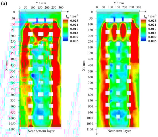
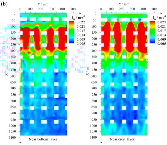
Figure 13.
Horizontal distribution of turbulence intensity in the near–bottom and near–crest vertical layers. (a) Single-row four-reef array; (b) dual-row eight-reef array.
The above findings suggest that smaller reef aspect ratios (Lr/hr = 3) lead to stronger but more localized vortex formations, which may enhance sediment scouring and local turbulence-driven mixing. Larger width-to-height ratios (Wr/hr > 1) promote a more extended vortex region, reducing the peak vorticity but distributing turbulence more uniformly, which may be beneficial for wave dissipation applications. Intermediate reef length ratios (Lr/hr = 4) suppress vortex formation, leading to lower turbulence intensity and potentially reducing the effectiveness of artificial reefs in modifying flow patterns. These results highlight the importance of selecting appropriate reef geometries based on the desired hydrodynamic function—whether maximizing localized turbulence for ecological enhancement or promoting a broader flow modification for coastal protection.
This study focuses on the hydrodynamic effects of artificial reefs under pure flow conditions. The research primarily investigates the fundamental hydrodynamic mechanisms in an idealized environment, without considering the influence of waves. Studying flow and turbulence under pure current conditions can avoid the complexity introduced by wave–current interactions [12]. The fundamental understanding obtained under pure current conditions can serve as a starting point for further research on wave–current interactions. For example, Li et al. [51] first established the baseline flow under wave-free conditions before gradually introducing wave effects when studying wave–current interactions. This approach helps to incrementally reveal the complex mechanisms of wave–current interactions. Moreover, numerous studies have shown that the presence of artificial reefs can alter wave propagation characteristics, reducing wave energy through reflection, refraction, and scattering, thereby protecting the coastline [52,53,54]. This interaction between waves and reefs is particularly significant in nearshore areas. Therefore, future work will address this limitation by incorporating wave–current interactions and sediment transport to provide a more comprehensive understanding of artificial reef performance. Additionally, ecological benefits and sediment dynamics will be explored to enhance the practical relevance of our findings.
4. Conclusions
This study combines Particle Image Velocimetry (PIV) experiments and numerical simulations to investigate the flow fields around single-row arrays of three and four reefs, as well as dual-row arrays of eight reefs. The research elucidates the intricate interactions between the configuration and dimensions of reef arrays and their hydrodynamic behavior, providing valuable insights for the design and optimization of artificial reef systems.
When the spacing ratio (d/lr)—where d is the longitudinal distance between adjacent reefs and lr is the length of a reef—is zero, the artificial reefs (ARs) are in close proximity. In this scenario, the flow resistance is primarily borne by the first reef block, which dominates the flow characteristics of the entire reef array. As d/lr exceeds 0.5, the number, size, and intensity of vortices within each reef block increase due to reduced inter-reef interactions and more pronounced vortex formation. The backflow generated behind the first two ARs is mitigated by the subsequent reefs. With increasing spacing, the wake flow behind the reef array develops more fully, resulting in a larger backflow region and an increase in the number and size of vortices. This greater spacing intensifies turbulence and reshapes the flow characteristics, with each reef block contributing uniquely to the overall flow pattern.
For a single-row, three-reef configuration with an aspect ratio Lr/hr (where Lr is the total length of the reef system and hr is the total height) of 3 and Wr/hr (where is the total width) of 0.68, the coverage and intensity of vortex dipoles reach their maximum within the reef array. A large clockwise vortex forms in the wake behind the array. When Lr/hr exceeds 3, the intensity of the vortex dipoles diminishes significantly. By adding a fourth reef to the array (Lr/hr = 4), the area of significant external turbulence expands, while strong internal turbulence remains confined behind the stoss face openings of the first reef block. Along the flow path, turbulence intensity decreases and is significantly reduced downstream of the reef array. Furthermore, the distance of the wake vortex from the leeside of the reef array increases as the spacing grows.
A comparison between single- and dual-row, four-reef arrays shows that increasing the width-to-height ratio (Wr/hr) leads to an expansion of the high-vorticity dipole region and the strongly turbulent area behind the stoss face. However, this also results in weakened turbulence downstream within the reef array.
This study provides a reference framework for the optimization of artificial reef configurations in coastal and ecological engineering. In coastal defense design, artificial reefs should be arranged with a larger spacing to enhance vortex intensity and reduce interference, thereby optimizing their flow characteristics. It is also recommended to set the reef length-to-height ratio to 3 and width-to-height ratio to 0.68 for a more appropriate vortex strength and flow distribution. However, this study focuses primarily on the hydrodynamic effects of ARs under simplified experimental conditions, whereas actual engineering applications involve more complex environments. Future research should investigate the impacts of ARs under combined random wave and current conditions to better simulate real-world scenarios. Prior research has also shown that the structural complexity of reefs and their wake regions can enhance fish abundance, biodiversity, and ecosystem functionality. These ecological factors should be incorporated into future studies to ensure a more comprehensive understanding of artificial reef performance.
Author Contributions
Conceptualization, C.K. and W.X.; methodology, C.K. and Y.Z.; software, Y.Z. and W.X.; validation, Y.Z., W.X. and X.C.; formal analysis, D.W.; investigation, Y.Z.; resources, C.K. and Y.Z.; data curation, Y.Z. and W.X.; writing—original draft preparation, W.X.; writing—review and editing, C.K., X.C., Q.Z. and W.X.; visualization, W.X. and D.W.; project administration, C.K. and Q.Z.; funding acquisition, C.K. and Q.Z. All authors have read and agreed to the published version of the manuscript.
Funding
This research was funded by the National Key Research and Development Program of China (No. 2022YFC3106205) and the National Natural Science Foundation of China (Grant No. 41976159 and 41776098). Professor Qingping Zou has been supported by the Natural Environment Research Council of the UK (Grant No. NE/V006088/1).
Data Availability Statement
Data are contained within the article.
Conflicts of Interest
The authors declare no competing financial interests or personal relationships that could influence this work.
References
- Reis, B.; Van Der Linden, P.; Pinto, I.S.; Almada, E.; Borges, M.T.; Hall, A.E.; Stafford, R.; Herbert, R.J.H.; Lobo-Arteaga, J.; Gaudêncio, M.J.; et al. Artificial Reefs in the North–East Atlantic Area: Present Situation, Knowledge Gaps and Future Perspectives. Ocean Coast. Manag. 2021, 213, 105854. [Google Scholar] [CrossRef]
- Paxton, A.B.; Peterson, C.H.; Taylor, J.C.; Adler, A.M.; Pickering, E.A.; Silliman, B.R. Artificial Reefs Facilitate Tropical Fish at Their Range Edge. Commun. Biol. 2019, 2, 168. [Google Scholar] [CrossRef]
- Vivier, B.; Dauvin, J.-C.; Navon, M.; Rusig, A.-M.; Mussio, I.; Orvain, F.; Boutouil, M.; Claquin, P. Marine Artificial Reefs, a Meta-Analysis of Their Design, Objectives and Effectiveness. Glob. Ecol. Conserv. 2021, 27, e01538. [Google Scholar] [CrossRef]
- Komyakova, V.; Chamberlain, D.; Jones, G.P.; Swearer, S.E. Assessing the Performance of Artificial Reefs as Substitute Habitat for Temperate Reef Fishes: Implications for Reef Design and Placement. Sci. Total Environ. 2019, 668, 139–152. [Google Scholar] [CrossRef] [PubMed]
- Rogers, A.; Blanchard, J.L.; Mumby, P.J. Vulnerability of Coral Reef Fisheries to a Loss of Structural Complexity. Curr. Biol. 2014, 24, 1000–1005. [Google Scholar] [CrossRef]
- Black, K.P.; Reddy, K.S.K.; Kulkarni, K.B.; Naik, G.B.; Shreekantha, P.; Mathew, J. Salient Evolution and Coastal Protection Effectiveness of Two Large Artificial Reefs. J. Coast. Res. 2020, 36, 709–719. [Google Scholar] [CrossRef]
- Ng, K.; Thomas, T.; Phillips, M.R.; Calado, H.; Borges, P.; Veloso-Gomes, F. Multifunctional Artificial Reefs for Small Islands: An Evaluation of Amenity and Opportunity for Sao Miguel Island, the Azores. Prog. Phys. Geogr. 2015, 39, 220–257. [Google Scholar] [CrossRef]
- Armono, H.D.; Hall, K.R. Wave Transmission on Submerged Breakwaters Made of Hollow Hemispherical Shape Artificial Reefs. In Proceedings of the Canadian Coastal Conference, Kingston, ON, Canada, 30 September–3 October 2003; pp. 1–13. [Google Scholar]
- Zheng, Y.H.; Kuang, C.P.; Han, X.J.; Ma, Y. Propagation Characteristics of Short Period Regular Wave over Perforated Reef-Type Submerged Breakwater Group. J. Tongji Univ. 2024, 52, 1227–1237. [Google Scholar] [CrossRef]
- Xia, X.; Li, Y.; Li, J.; Gong, P.H.; Huang, J.L.; Lu, J.K. Effect of Oyster Shell Filling in Artificial Reefs on Flow Field Environment and Assessing the Potential of Carbon Fixation. J. Sea Res. 2024, 202, 102537. [Google Scholar] [CrossRef]
- Chen, X.L.; Che, X.; Zhou, Y.; Tian, C.F.; Li, X.F. A Numerical Simulation Study and Effectiveness Evaluation on the Flow Field Effect of Trapezoidal Artificial Reefs in Different Layouts. J. Mar. Sci. Eng. 2023, 12, 3. [Google Scholar] [CrossRef]
- Guo, C.L.; Zhu, L.X.; Liang, Z.L.; Xie, W.D.; Zheng, Y.J.; Tang, Y.L.; Jiang, Z.Y. Study on the Effect of Internal Reefs Deflection on the Flow Field Effect of Unit Reef. Ocean Eng. 2023, 286, 115653. [Google Scholar] [CrossRef]
- Zheng, Y.H.; Kuang, C.P.; Zhang, J.B.; Gu, J.; Chen, K.; Liu, X. Current and Turbulence Characteristics of Perforated Box-Type Artificial Reefs in a Constant Water Depth. Ocean Eng. 2022, 244, 110359. [Google Scholar] [CrossRef]
- Kuang, C.; Li, H.; Zheng, Y.; Xing, W.; Cong, X.; Chen, J. Turbulent Characteristics of a Submerged Reef under Various Current and Submergence Conditions. J. Mar. Sci. Eng. 2024, 12, 214. [Google Scholar] [CrossRef]
- Lowe, R.J.; Altomare, C.; Buckley, M.L.; Da Silva, R.F.; Hansen, J.E.; Rijnsdorp, D.P.; Domínguez, J.M.; Crespo, A.J.C. Smoothed Particle Hydrodynamics Simulations of Reef Surf Zone Processes Driven by Plunging Irregular Waves. Ocean Model. 2022, 171, 101945. [Google Scholar] [CrossRef]
- Wang, M.Z.; Pan, Y.; Shi, X.K.; Wu, J.L.; Sun, P.N. Comparative Study on Volume Conservation among Various SPH Models for Flows of Different Levels of Violence. Coast. Eng. 2024, 191, 104521. [Google Scholar] [CrossRef]
- Maslov, D.; Pereira, E.; Duarte, D.; Miranda, T.; Ferreira, V.; Tieppo, M.; Cruz, F.; Johnson, J. Numerical Analysis of the Flow Field and Cross Section Design Implications in a Multifunctional Artificial Reef. Ocean Eng. 2023, 272, 113817. [Google Scholar] [CrossRef]
- Pan, Y.; Tong, H.; Wei, D.; Xiao, W.; Xue, D. Review of Structure Types and New Development Prospects of Artificial Reefs in China. Front. Mar. Sci. 2022, 9, 853452. [Google Scholar]
- Guo, Y.; Qin, C.X.; Zhang, S.Y. Flow Field Effect of Cube Reef Monocase of Different Structure. Prog. Fish. Sci. 2022, 43, 1–10. [Google Scholar] [CrossRef]
- Fang, J.H.; Lin, J.; Yang, W.; Wen, Y.; Qi, F.Q. Numerical Simulation of Flow Field Effect around the Double-Layer Cross-Wing Artificial Reef. J. Shanghai Ocean Univ. 2021, 30, 743–754. [Google Scholar]
- Liu, X.M.; Zheng, Y.N.; Chen, C.P.; Tian, C.F. Numerical Simulation of Flow around Frame and Caisson Artificial Reef Models. J. Dalian Ocean Univ. 2019, 34, 133–138. [Google Scholar] [CrossRef]
- Zheng, Y.X.; Guan, C.T.; Song, X.F.; Liang, Z.L.; Cui, Y.; Li, Q. Numerical Simulation on Flow Field around Star Artificial Reefs. Trans. Chin. Soc. Agric. Eng. 2012, 28, 185–193 + 297–298. [Google Scholar]
- Xi, Y.; Tian, T.; Yang, J.; Wu, Z.X.; Liu, M.; Gao, D.K.; Chen, Y. Reef Approaching Behavior of Juvenile Sebastes Schlegeli under Different Flow Fields. J. Dalian Fish. Univ. 2020, 35, 399–406. [Google Scholar] [CrossRef]
- Folpp, H.; Lowry, M.; Gregson, M.; Suthers, I.M. Fish Assemblages on Estuarine Artificial Reefs: Natural Rocky-Reef Mimics or Discrete Assemblages? PLoS ONE 2013, 8, e63505. [Google Scholar] [CrossRef]
- Lai, J.L.; Yang, F.F.; Huang, D.Z.; Huang, S.Q.; Sun, X.J. Artificial Reef Design and Flow Field Analysis for Enhancing Stichopus Japonicus Cultivation in Haizhou Bay. J. Mar. Sci. Eng. 2024, 12, 1130. [Google Scholar] [CrossRef]
- Gomes, A.; Pinho, J.L.S.; Valente, T.; Antunes do Carmo, J.S.; Hegde, A. Performance Assessment of a Semi-Circular Breakwater through CFD Modelling. J. Mar. Sci. Eng. 2020, 8, 226. [Google Scholar] [CrossRef]
- Wang, J.H.; Liu, L.L.; Cai, X.C.; Chen, J.Y.; Yang, Y.X.; Jiang, S.X. Numerical Simulation Study on Influence of Disposal Space on Effects of Flow Field Around Porous Square Artificial Reefs. Prog. Fish. Sci. 2020, 41, 40–48. [Google Scholar] [CrossRef]
- Zhang, J.T.; Zhu, L.X.; Liang, Z.L.; Sun, L.Y.; Nie, Z.Y.; Wang, J.H.; Xie, W.D.; Jiang, Z.Y. Numerical Study of Efficiency Indices to Evaluate the Effect of Layout Mode of Artificial Reef Unit on Flow Field. J. Mar. Sci. Eng. 2021, 9, 770. [Google Scholar] [CrossRef]
- Liu, T.-L.; Su, D.-T. Numerical Analysis of the Influence of Reef Arrangements on Artificial Reef Flow Fields. Ocean Eng. 2013, 74, 81–89. [Google Scholar] [CrossRef]
- Mao, H.Y.; Hu, C.; Yu, D.Y.; Wang, K.R. Optimization study of diversion reef assemblage based on the numerical simulation of flow field. J. Xiamen Univ. Nat. Sci. 2022, 61, 723–730. [Google Scholar] [CrossRef]
- Lin, M.J.; Ji, X.R.; Wang, F.X. Flow field effects and hydrodynamic analysis of square composite reefs. Nat. Sci. J. Hainan Univ. 2022, 40, 66–75. [Google Scholar] [CrossRef]
- Zheng, Y.X.; Liang, Z.L.; Guan, C.T.; Song, X.F.; Li, J.; Cui, Y.; Li, Q.; Shan, X.L.; Xu, W.W. Numerical simulation and experimental study on flow field of artificial reefs in three tube-stacking layouts. Oceanol. Limnol. Sin. 2014, 45, 11–19. [Google Scholar]
- Kim, D.; Jung, S.; Na, W.-B. Evaluation of Turbulence Models for Estimating the Wake Region of Artificial Reefs Using Particle Image Velocimetry and Computational Fluid Dynamics. Ocean Eng. 2021, 223, 108673. [Google Scholar] [CrossRef]
- Li, J.; Zheng, Y.; Gong, P.; Guan, C. Numerical Simulation and PIV Experimental Study of the Effect of Flow Fields around Tube Artificial Reefs. Ocean Eng. 2017, 134, 96–104. [Google Scholar] [CrossRef]
- Tan, S.F.; Wang, X.Z.; Zhang, M.L.; Liu, C.G.; Wang, A.M.; Xu, X.F.; Xu, P. Flow field effect of cuboid frame artificial reef. Chin. J. Appl. Mech. 2023. Available online: http://kns.cnki.net/kcms/detail/61.1112.o3.20230227.1445.020.html (accessed on 1 February 2025).
- Zou, Q.; Peng, Z. Evolution of Wave Shape over a Low-Crested Structure. Coast. Eng. 2011, 58, 478–488. [Google Scholar] [CrossRef]
- Chaput, R.; Majoris, J.E.; Buston, P.M.; Paris, C.B. Hydrodynamic and Biological Constraints on Group Cohesion in Plankton. J. Theor. Biol. 2019, 482, 109987. [Google Scholar] [CrossRef]
- Shu, A.; Zhang, Z.; Wang, L.; Sun, T.; Yang, W.; Zhu, J.; Qin, J.; Zhu, F. Effects of Typical Artificial Reefs on Hydrodynamic Characteristics and Carbon Sequestration Potential in the Offshore of Juehua Island, Bohai Sea. Front. Environ. Sci. 2022, 10, 979930. [Google Scholar] [CrossRef]
- Jiang, Z.Y. Numerical Simulation of Hydrodynamics for Artificial Reefs. Ph.D. Thesis, Ocean University of China, Qingdao, China, 2009. [Google Scholar]
- Kuang, C.P.; Zheng, Y.H.; Gu, J.; Han, X.J. Simulation methods of inner flow field and flow characteristics induced by perforated reef-type breakwater. J. Tongji Univ. 2023, 51, 1073–1084. [Google Scholar]
- Kuang, C.P.; Pan, Y.; Zhang, Y.; Liu, S.G.; Yang, Y.X.; Zhang, J.B.; Dong, P. Performance Evaluation of a Beach Nourishment Project at West Beach in Beidaihe, China. J. Coast. Res. 2011, 27, 769–783. [Google Scholar] [CrossRef]
- Ma, Y. Experimental Investigation on Beach Profile Evolution Process with Offshore Interventions of Artificial Reef and Submerged Sand Bar. Ph.D. Thesis, Tongji University, Shanghai, China, 2020. [Google Scholar]
- Zou, Q. A Viscoelastic Model for Turbulent Flow over Undulating Topography. J. Fluid Mech. 1998, 355, 81–112. [Google Scholar] [CrossRef]
- Launder, B.E.; Spalding, D.B. The Numerical Computation of Turbulent Flows. Comput. Methods Appl. Mech. Eng. 1974, 3, 269–289. [Google Scholar] [CrossRef]
- Chen, H.; Zou, Q. Characteristics of Wave Breaking and Blocking by Spatially Varying Opposing Currents. J. Geophys. Res. Ocean 2018, 123, 3761–3785. [Google Scholar] [CrossRef]
- Shih, T.-H.; Liou, W.W.; Shabbir, A.; Yang, Z.G.; Zhu, J. A New K-ϵ Eddy Viscosity Model for High Reynolds Number Turbulent Flows. Comput. Fluids 1995, 24, 227–238. [Google Scholar] [CrossRef]
- van Heijst, G.J.F.; Flór, J.B. Dipole Formation and Collisions in a Stratified Fluid. Nature 1989, 340, 212–215. [Google Scholar] [CrossRef]
- Pope, S.B. Turbulent Flows, 1st ed.; Cambridge University Press: Cambridge, UK, 2000; ISBN 9780521598866. [Google Scholar]
- Gutmark, E.J.; Ibrahim, I.M.; Murugappan, S. Dynamics of Single and Twin Circular Jets in Cross Flow. Exp. Fluids 2011, 50, 653–663. [Google Scholar] [CrossRef]
- Srineash, V.K.; Murali, K. Functional Performance of Modular Porous Reef Breakwaters. J. Hydro-Environ. Res. 2019, 27, 20–31. [Google Scholar] [CrossRef]
- Li, Y.; Zheng, Y.; Lin, Z.; Adcock, T.A.A.; Bremer, T.S. van den Surface Wavepackets Subject to an Abrupt Depth Change. Part 1. Second-Order Theory. J. Fluid. Mech. 2021, 915, A71. [Google Scholar] [CrossRef]
- Kim, T.; Kwon, Y.; Lee, J.; Lee, E.; Kwon, S. Wave Attenuation Prediction of Artificial Coral Reef Using Machine-Learning Integrated with Hydraulic Experiment. Ocean Eng. 2022, 248, 110324. [Google Scholar] [CrossRef]
- Xing, W.; Kuang, C.; Li, H.; Chen, J.; Shi, L.; Zou, Q. Effect of Open-Area Ratios on Wave Attenuation over a Submerged Reef Breakwater: An Experimental Study. Ocean Eng. 2024, 312, 119221. [Google Scholar] [CrossRef]
- Van Gent, M.R.A.; Buis, L.; Van Den Bos, J.P.; Wüthrich, D. Wave Transmission at Submerged Coastal Structures and Artificial Reefs. Coast. Eng. 2023, 184, 104344. [Google Scholar] [CrossRef]
Disclaimer/Publisher’s Note: The statements, opinions and data contained in all publications are solely those of the individual author(s) and contributor(s) and not of MDPI and/or the editor(s). MDPI and/or the editor(s) disclaim responsibility for any injury to people or property resulting from any ideas, methods, instructions or products referred to in the content. |
© 2025 by the authors. Licensee MDPI, Basel, Switzerland. This article is an open access article distributed under the terms and conditions of the Creative Commons Attribution (CC BY) license (https://creativecommons.org/licenses/by/4.0/).