Flood Regional Composition Considering Typical-Year and Multi-Site Flood Source Characteristics

Abstract

The construction and operation of reservoirs have significantly altered the downstream flow regime, and the flood regional composition (FRC) method has been widely used to estimate design flood considering the regulation impact of upstream cascade reservoirs. This paper proposes a novel flood regional composition based on the proper orthogonal decomposition (FRC-POD) method that comprehensively takes into account typical-year flood differences and the multi-site flood source characteristics. The proposed method is applied at Cuntan hydrologic station in the upper Yangtze River and compared with the typical-year flood composition (TYFC) method and the most likely flood regional composition (MLFRC) method. The results show the following: (1) The proposed FRC-POD method can identify main flood sources in the design section and pay more attention to floods from the mainstream and the uncontrolled interval basin. (2) Compared with the originally designed values, the 1000-year design peak discharge and 3 d, 7 d, and 15 d flood volumes estimated by the FRC-POD method are decreased by 41.3%, 40.2%, 36.6%, and 34.7%, respectively. (3) Current FRC methods depend on the selected typical-year flood events and have several solutions, while the proposed method has only one final solution, which is more reasonable in practical application. (4) A comparative study proves that the FRC-POD method could obtain rational design flood estimation and is worth further study.

1. Introduction

Reservoir is an important engineering measure for water resource management and has many functions, such as flood control, hydropower generation, water supply, irrigation, and so on [1]. In recent decades, a large number of reservoirs have been built and operated in the world to meet socioeconomic development. The construction and operation of these reservoirs have significantly changed the downstream hydrological regime and impacted design flood estimation [2].

Traditional design flood estimation mainly concentrates on the analysis of annual maximum peak discharge or flood volumes, in which the frequencies of the peak discharge or flood volumes corresponding with design return periods are estimated. However, information about the peak, duration, and volume of the critical flood event is essential for water resource planning and management, which requires the comprehensive description of the whole flood event rather than only the peak discharge or flood volume derived by the traditional flood frequency analysis method [3]. The flood hydrograph with the highest peak discharge or the largest flood volume is usually selected as a typical-year flood hydrograph (TFH) [4], and the design flood hydrograph (DFH) is derived by multiplying each discharge ordinate of the TFH by an amplifier that is either the ratio of the design peak discharge or flood volume with that of a given return period [5].

According to the Chinese guideline “Regulation for calculating design flood of water resources and hydropower projects” [6], when there is a reservoir with large storage in the upstream of the design section or when the reservoir has a flood control task for the downstream, flood regional composition (FRC) analysis in the downstream design section should be carried out. The FRC method based on the mechanism of runoff generation and flow routing from different sub-basins or regions can estimate design floods considering the regulation influences of upstream reservoirs. The downstream flow discharge at the design section is regarded as the combination of inter-basin inflow and outflow discharge transformed by man-made reservoir operation rules. Generally, the characteristics of the reservoirs (e.g., storage capacity and operation rules) and the flood proportion of sub-basins make a great difference on downstream design floods. In the traditional FRC framework, the design flood is investigated with the natural flood frequency curve and design probability p, and searches for the appropriate combination of flood volumes among each sub-basin in the natural condition. Then, the natural TFH is selected and the corresponding DFH at the sub-basins can be derived using the amplifier of their flood volumes [5]. Finally, the downstream design flood considered the influence of upstream reservoirs can be obtained through flow routing and complex reservoir operation, which meanwhile maintains same probability p as that of the natural condition in the planning and construction periods. Obviously, the FRC framework could fully consider reservoir regulation, reasonably allocate the flood volumes between the upstream reservoir and the inter-basin of adjacent reservoirs, and input the combination schemes into the cascade reservoir system to obtain the design flood of downstream sections.

The Ministry of Water Resources recommended two basic FRC methods [6]: i.e., the typical-year flood composition (TYFC) method and equivalent frequency regional composition (EFRC). The TYFC method first selects several representative and large flood events that are unfavorable to flood prevention in the design section and then analyzes flood volumes for each sub-basin under a specific design frequency. The corresponding flood volume in each sub-basin is allocated and amplified according to the ratio between the total flood volume at the downstream section with design probability p and that in the typical-year flood hydrograph. The TYFC method is simple and intuitive and has been commonly used in engineering design, particularly suitable for the situation of many sub-basins with complicated flood compositions. However, the design floods estimated by the TYFC method are subjective and uncertain, since there are many different frequencies among the upstream and downstream flood events for a selected typical-year flood hydrograph. Thus, how to choose the appropriate typical-year flood event is the key problem in engineering practice. If the selected typical-year flood event does not reflect the real FRC law, then the estimated design flood has large uncertainty.

The EFRC method [6] assumes that the exceedance probability of design flood occurring at upstream reservoir site or interval basin is identical with that of the downstream design section, i.e., it is implicitly assumed that the upstream reservoir and interval basin flow data series are fully correlated. However, the relationship of the upstream reservoir and interval basin flow data series is usually divergent from this assumption in real cases, which questions the feasibility of the EFRC method, leading to biased design flood estimation [3]. The implementation of the EFRC method is very complex when the number of cascade reservoirs is more than 3. The number of EFRC schemes (2ⁿ) increases exponentially as the number of reservoirs increases (n). In addition, the selection of composition schemes may vary with different individuals [7].

The most likely flood regional composition (MLFRC) method proposed by Guo et al. in 2018 [3] assumes that FRCs may differ in terms of occurrence likelihood and can be measured by the joint probability density function of floods occurring at all sub-basins [8]. The joint probability density function is established based on the copula theory [9,10], via which the association between floods of different sub-basins can be represented. The MLFRC method selects the FRC with the largest occurrence likelihood as the only solution.

Since the flood regional composition is a random event, both the TYFC and EFRC methods are based on simplified assumptions to give the relationship between floods in each sub-basin, which are unscientific and unreasonable. The TYFC method can only select the flood hydrograph of a certain year for analysis and calculation and is unable to consider other flood regional compositions of different years, whose results have certain subjectivity and uncertainty [11,12]. The EFRC method assumes that the flow data series of the upstream reservoir or inter-basin is completely correlated with the flow data series at the downstream section, and whether it complies with the law of flood regional composition depends on the correlation between that sub-basin and the design section [13]. Since the runoff generation and flood routing mechanism have changed due to the flood regulation impact of upstream reservoirs, none of TYFC, EFRC, and MLFRC methods can take into account the multi-site flood source characteristics. Therefore, there is an urgent need for an objective and reasonable flood regional composition method that can consider typical-year and multi-site flood source characteristics.

The proper orthogonal decomposition (POD) method has been widely applied in the extraction of discrete data feature information. Inspired by this, the POD method is introduced for flood regional composition analysis, which can extract dominant paradigms of the typical-year flood events. This paper proposes a novel flood regional composition based on the proper orthogonal decomposition (FRC-POD) method that integrates the multi-site flood sources and fully considers typical-year characteristics. The proposed FRC-POD method is applied in the upper Yangtze River to estimate design flood at Cuntian hydrologic station that is the inflow control station of Three Gorges Reservoir. The performance of the FRC-POD method is compared with the current TYFC and MLFRC methods. The structure of this paper is as follows: The current FRC methods are briefly introduced in Section 2. A novel FRC-POD method is proposed in Section 3. Section 4 reports study data in the upper reach of Yangtze River basin in China. Section 5 provides the case study results and discussions. Section 6 summarizes the conclusions.

2. Current Flood Regional Composition Methods

Figure 1 shows the sketch diagram of cascade reservoirs in a river basin, where there are n cascade reservoirs. A_i, B_i, and C represent the ith upstream reservoir, the ith interval basin, and the design section, respectively. The random variables X_i, Y_i, and Z represent the inflow of A_i, B_i, and C with corresponding values x_i, y_i, and z, respectively.

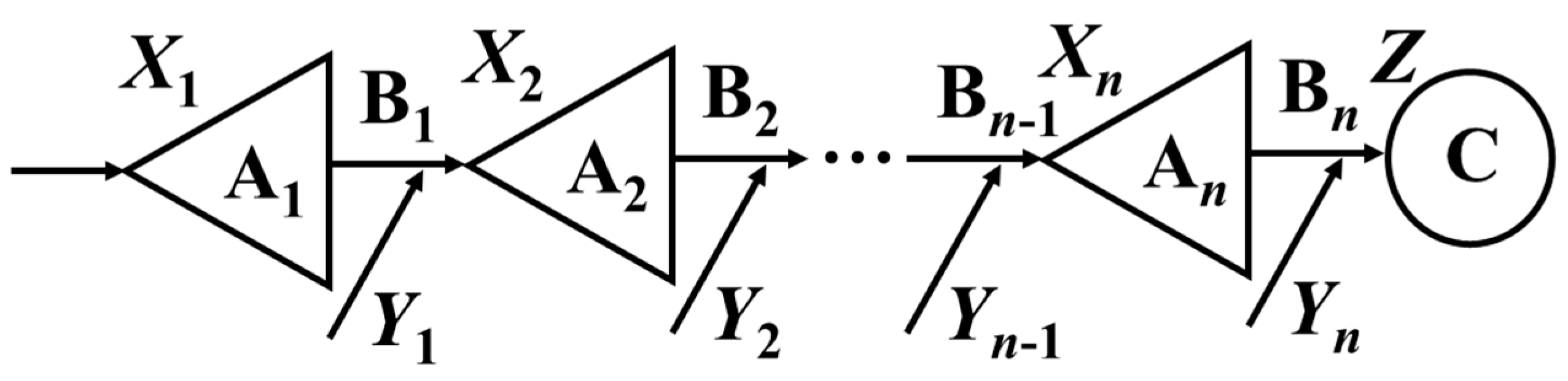
2.1. Typical-Year Composition (TYFC) Method

Typical-year flood composition (TYFC) method selects several representative flood events, which are unfavorable to flood prevention in the design section [6]. When the reservoir storage capacity is large, the flood volume is more significant than peak discharge in reservoir flood control operation. According to the typical-year flood volume in each sub-basin, the DFH can be derived with the TFH amplified by the ratio of their flood volume. The magnification ratio can be controlled according to design flood volume and the typical-year flood volume as follows:

$$K_{wt}={\displaystyle \frac{W_{tp}}{W_t}}$$

(1)

where W_tp and $W_t$ are the design flood volume and the typical-year flood volume at time period t, respectively K_wt is the amplification coefficient for volume-based control.

2.2. Equivalent Frequency Regional Composition (EFRC) Method

The EFRC method recommended by the Ministry of Water Resources [6] has been widely used in China. The principle of the EFRC method was described in detail by Guo et al. [3].

2.3. Most Likely Regional Composition (MLFRC) Method

The MLFRC method assumes that FRCs may differ in terms of their probability of occurrence [3], which can be measured by the value of joint probability density function (PDF) of random variables X₁, X₂, …, X_n, Z, i.e., f(x₁, x₂, …, x_n, z). According to Sklar’s theorem [14], the joint PDF can be expressed by its marginal distributions and the copula function as follows [15]:

$$f(x_1,x_2,\cdots ,x_{n-1},x_n,z)=c(u_1,u_2,\dots ,u_{n-1},u_n,v){\displaystyle \prod _{i=1}^n{f}_{X_i}(x_i)·f_Z(z)}$$

(2)

where c is the copula function; u₁, u₂, …, u_n, v are the corresponding cumulative frequencies of x₁, x₂, …, x_n, z, respectively.$f_{X_i}(x_i)$ (i = 1, 2, …, n) and $f_Z(z)$ are the marginal distributions at reservoirs A₁, A₂… A_n and downstream design section C, respectively.

The composition (x₁, x₂, …, x_n, z) is more likely to occur with the increase in PDF f(x₁, x₂, …, x_n, z). The f(x₁, x₂, …, x_n, z) in Equation (2) is maximized with water balance constraints by the following equation:

$$\begin{array}{cc}\hfill max& f(x_1,x_2,\cdots ,x_{n-1},x_n,z)=c(u_1,u_2,\dots ,u_{n-1},u_n,v){\displaystyle \prod _{i=1}^n{f}_{X_i}(x_i)·f_Z(z)}\hfill \\ \hfill s.t.& \left\{\begin{array}{l}{x}_1+y_1=x_2\\ x_1+y_1+y_2=x_3\\ \dots \\ x_1+y_1+y_2+\dots +y_n=z\end{array}\right.\hfill \end{array}$$

(3)

where z is the design flood volume of the investigated design site for a given return period.

The joint PDF f(x₁, x₂, …, x_n, z) in Equation (3) is maximized when its first order derivative equals zero. Guo et al. [3] show the derivation procedures of MLFRC method in detail. Xiong et al. [7,8] proposed a genetic algorithm (GA)-based strategy to solve Equation (3) and obtain the final solution for a high dimensional cascade reservoir system.

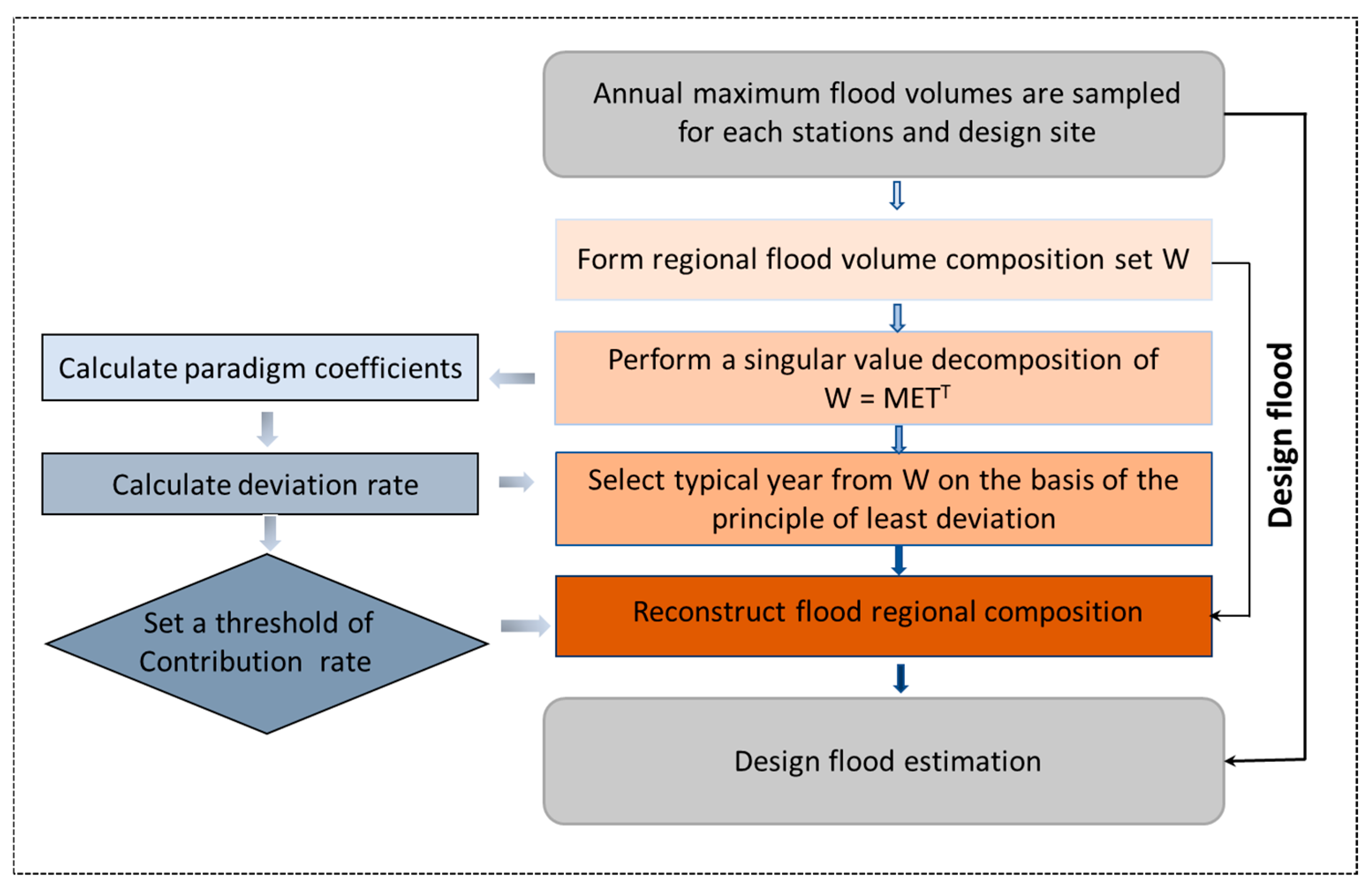
3. Proposed Novel FRC-POD Method

The current FRC methods cannot take into account the typical-year flood events and multi-site flood source characteristics. This section will introduce a novel flood regional composition based on the proper orthogonal decomposition (FRC-POD) method.

3.1. Proper Orthogonal Decomposition (POD)

Proper orthogonal decomposition (POD) is a widely used dimensionality reduction tool that can decompose data series into orthogonal basis functions and then extract sufficient basis functions to describe the original data series optimally [16]. The POD method has been derived independently by various individuals and consequently takes a variety of names in different research fields, e.g., Karhunen–Loève decomposition [17], singular value decomposition (SVD), and principal components analysis [18]. Because of ease of interpretation and its broad applicability to data series from both simulations and experiments [19], the POD technique has been widely used in many research fields, such as fluid mechanics, aerodynamics, economics, statistics, psychology, etc. POD can be considered as fitting an n-dimensional ellipsoid to the data series, where each axis is represented by spatially orthogonal eigenvectors computed using a covariance matrix built from the dataset [20]. For example, Higham et al. [18] used modal decompositions to explain the sudden expansion of the mixing layer in the wake of a groyne in a shallow flow. Feeny and Liang [21] extracted mode shapes of a structure by implementing POD in measured response data. Since flood routing and the propagation process change continuously over time and space, the POD method has potential applications in the FRC analysis for design flood estimation.

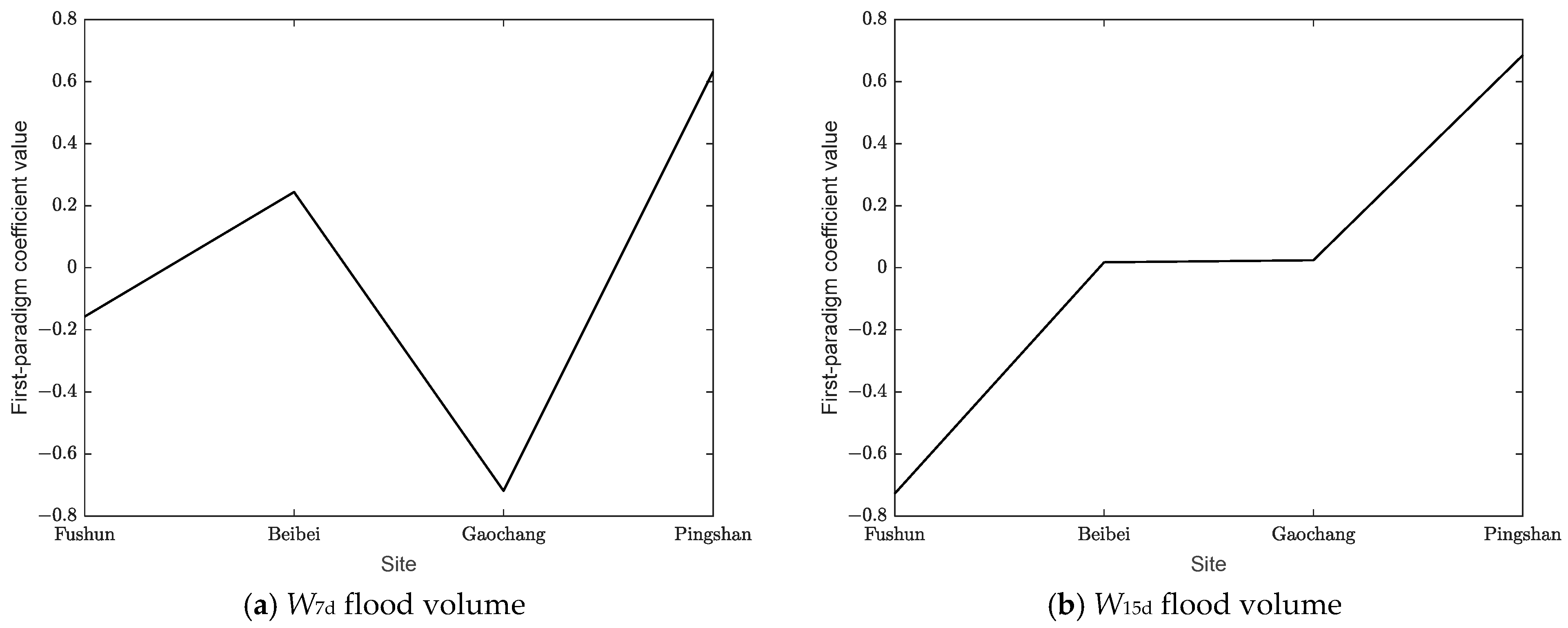
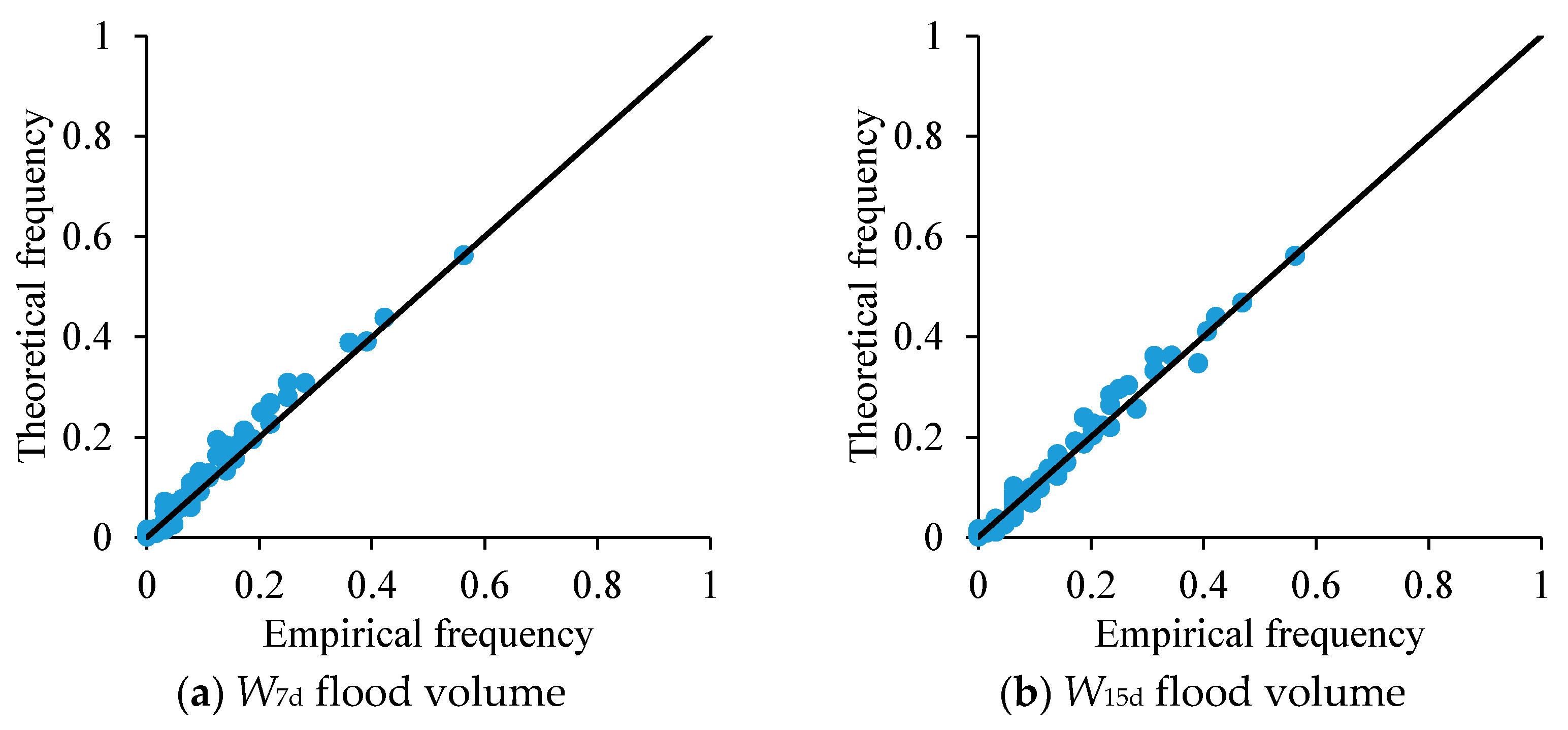
3.2. Flood Regional Composition Based on POD

The flow chart of the proposed FRC-POD method is shown in Figure 2. The main estimation procedures are the following steps:

(1) The observed daily flow data series at the design site and upstream hydrologic stations are collected. The annual maximum flood volume data series at design site and upstream hydrologic stations corresponding to the occurrence date of the annual maximum flood volume at design site are sampled. Then, the design flood volume for the given return period at the design site is estimated by the flood frequency analysis method based on the restored natural flood data series.

(2) The corresponding flood volumes occurring in each sub-basin are obtained to form the regional flood volume set W_m,n after subtracting the average value of flood volumes for all sub-basins in the same year.

$$\left\{\begin{array}{c}{\mathrm{W}}_{m,n}=\left[\begin{array}{cccc}{w}_{1,1}& w_{1,2}& \dots & w_{1,n}\\ w_{2,1}& w_{2,2}& \dots & w_{2,n}\\ \dots & \dots & \dots & \dots \\ w_{m,1}& w_{m,2}& \dots & w_{m,n}\end{array}\right]\\ w_{i,j}=v_{i,j}-{\displaystyle \sum _{a=1}^n\frac{v_{i,a}}{n}}\end{array}\right.$$

(4)

where m is the total number of years; $n$ is the total number of sub-basins; and v_i,j denotes the flood volume at site i in j year.

(3) The regional flood volume set W_m,n in Equation (5) performs singular value decomposition. Transform variables that may be correlated into linearly uncorrelated variables through orthogonal transformation as follows:

$${\mathrm{W}}_{m,n}={\mathrm{M}}_{m,m}{\mathrm{E}}_{m,n}{\mathrm{T}}_{n,n}^{\mathrm{T}}$$

(5)

where M_m,m and T_n,n are the standard orthonormal eigenvector sets of WW^T and W^TW, which are also named as left and right singular matrix, respectively; E_m,n = diag($\sqrt{{\lambda }_1},\sqrt{{\lambda }_2},\dots ,\sqrt{{\lambda }_n}$) $({\lambda }_1>{\lambda }_2>\dots >{\lambda }_n>0)$ is the matrix of singular value, where λ_i is the ith eigenvalue of W^TW.

Replace each standard orthonormal vector of T_n,n as T_i.

$$\left\{\begin{array}{c}{\mathrm{T}}_{n,n}=\left[{\mathrm{T}}_1,{\mathrm{T}}_2,\dots ,{\mathrm{T}}_n\right]=\left[\begin{array}{cccc}{t}_{1,1}& t_{1,2}& \dots & t_{1,n}\\ t_{2,1}& t_{2,2}& \dots & t_{2,n}\\ \dots & \dots & \dots & \dots \\ t_{n,1}& t_{n,2}& \dots & t_{n,n}\end{array}\right]\\ {\mathrm{T}}_i={[t_{1,i},t_{2,i},\dots ,t_{n,i}]}^{\mathrm{T}}\end{array}\right.$$

(6)

Then, T_i is the ith paradigm coefficient of W_m,n, whose energy contribution rate is calculated by the following:

$$C_i={\displaystyle \frac{{\lambda }_i}{{\displaystyle \sum _{i=1}^n{\lambda }_i}}}$$

(7)

where C_i indicates the magnitude of T_i’s influence on the flood composition at the design site. If the paradigm coefficients T₁, T₂, …T_k whose cumulative flood contribution rate is larger than a predetermined threshold at the design site, then they are selected as the dominant paradigms. The first paradigm has the largest contribution rate.

(4) Calculate the deviation rate R_i between observed flood volume at the design site in the ith year and the first paradigm coefficient T₁, and selected flood volume that is the closest to the first paradigm coefficient based on the principle of the minimum deviation rate R_i, which is calculated as follows:

$$R_i={{\displaystyle \sum _{i=1}^n(\frac{t_{i,1}}{{\displaystyle \sum _{\mathrm{j}=1}^n\frac{t_{j,1}}{n}}}-\frac{v_{r,i}}{{\displaystyle \sum _{j=1}^n\frac{v_{r,j}}{n}}})}}^2$$

(8)

(5) Assuming that the flood’s composition in lth year [$v_{l,1},v_{l,2},\dots ,v_{l,n}$] has the minimum deviation rate, then reconstruction flood regional composition FRC = [frc₁, frc₂, ... , frc_n] is given as follows:

$$fr{c}_i={\displaystyle \sum _{j=1}^n\frac{v_{l,j}}{n}}+{\displaystyle \sum _{j=1}^k\frac{C_j}{R_j}{m}_{l,i}·t_{i,j}}$$

(9)

where m_l,i is the element of M_m,m in line l colume i.

(6) The design flood regional compositions for the study region are obtained by amplifying the reconstruction FRC results calculated by Equation (9) with the corresponding flood volume by Equation (1).

4. Study Region and Data

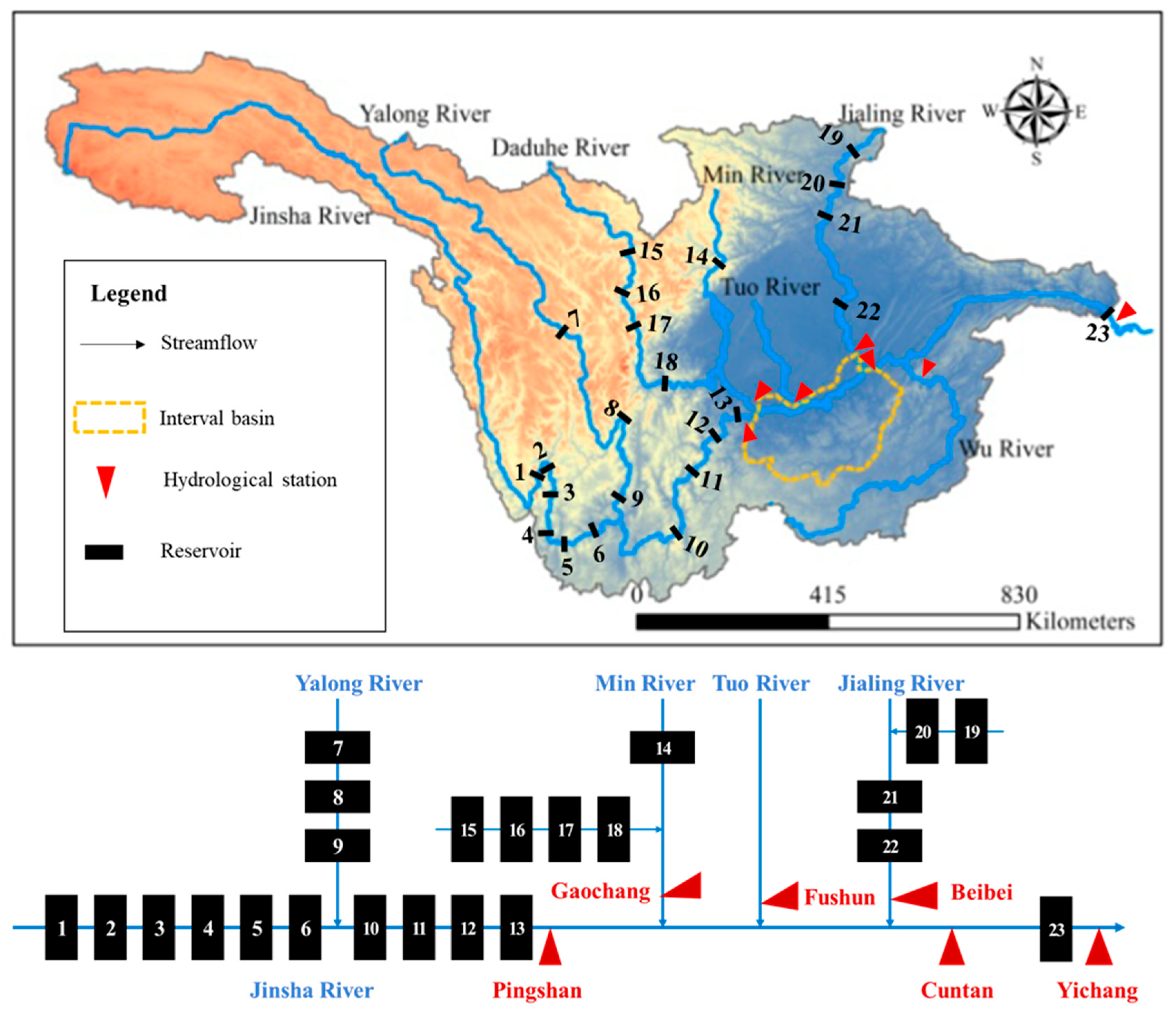
4.1. The Upper Yangtze River Basin

The Yangtze River is the largest basin in China with a drainage area of 1.8 million km². The upper Yangtze River flows from the river source to the Yichang City of Hubei Province with a length of about 4504 km and a catchment area about 1 million km². Figure 3 shows the sketch map of the upper Yangtze River basin and the investigated hydrologic stations and reservoirs, where the Jinsha River is the mainstream in the upper reach of the Yangtze River, while the Min River, Tuo River, Jialin River, and Wu River are the main tributaries. The Pingshan, Gaochang, Fushun, and Beibei hydrologic stations are the outlet of the Jinsha River, Min River, Tuo River, and Jialin River, respectively.

There are many large-scale reservoirs that have been built in recent decades with a total storage capacity of 150 billion m³ in the upper Yangtze River basin. As shown in Figure 3, there are 23 large-scale controlling reservoirs in the upper Yangtze River basin. These reservoirs serve essential roles in flood control, hydropower generation, navigation, and ecosystem maintenance in the Yangtze River basin [22].

Table 1. Characteristic parameters of 23 major controlling reservoirs in upper Yangtze River basin.

Reservoir Name	Reservoir Number	Catchment Area (104 km2)	Normal Pool Level (m)	Total Storage (108 m3)	Regulation Storage (108 m3)	Flood Prevention Storage (108 m3)	Installed Hydropower Capacity (GW)	Operation Year
Liyuan	1	22.00	1618	8.05	1.73	1.73	2.40	2016
Ahai	2	23.54	1504	8.85	2.38	2.15	2.00	2014
Jinanqiao	3	23.74	1418	9.13	3.46	1.58	2.40	2012
Longkaikou	4	24.00	1298	55.8	11.3	12.6	1.80	2014
Ludila	5	24.73	1223	17.18	3.76	5.64	2.16	2014
Guanyinyan	6	25.65	1134	22.5	5.55	5.42	3.00	2016
Lianghekou	7	6.57	2865	108	65.6	21.44	3.00	2022
Jinping-I	8	10.26	1880	79.9	49.11	16.0	3.60	2014
Ertan	9	11.64	1200	58	33.7	9.0	3.30	1999
Wudongde	10	40.61	975	74.08	30.2	24.4	10.20	2021
Baihetan	11	43.03	825	206.27	104	75	16.00	2022
Xiluodu	12	45.44	600	126.7	64.6	46.5	12.60	2014
Xiangjiaba	13	45.88	380	51.63	9.03	9.03	6.00	2014
Zipingpu	14	2.27	877	11.12	7.74	1.67	0.76	2006
Houziyan	15	5.40	1842	7.06	3.87	3.87	0.17	2017
Changheba	16	5.67	1690	10.75	4.15	4.15	0.26	2017
Dagangshan	17	6.23	1130	7.42	1.17	1.17	0.26	2015
Pubugou	18	7.74	850	53.9	38.82	10.56	0.36	2010
Bikou	19	2.60	704	2.17	1.46	1.56	0.30	1997
Baozhusi	20	2.84	588	25.5	13.4	2.8	0.70	1998
Tingzikou	21	6.11	458	40.67	17.32	14.4	1.10	2014
Caojie	22	15.61	203	22.18	0.65	1.99	0.50	2011
TGR	23	100.0	175	393	278.94	221.5	22.5	2008

lists the characteristic parameters of the 23 major controlling reservoirs in the upper Yangtze River basin.

The Cuntan hydrologic station is selected as the design site in this case study, and it is the inflow control station of the Three Gorges Reservoir (TGR) that is the biggest multi-purpose water conservancy project around the world. As shown in Table 1, the total storage capacity of TGR is 39.3 billion m³ (22.15 billion m³ for flood prevention storage), which can effectively mitigate flood risks at the downstream Jingjiang River reach and Chenglingji control section, which has suffered from frequent and disastrous flood damages in history. The TGR has a firm output of 4990 MW with a total of 22.5 GW of installed hydropower capacity and generates 86 billion kW·h hydropower annually.

As shown in Figure 3, the flood at Cuntan station mainly originates from Jinsha River (Pingshan station), Min River (Gaochang station), Tuo River (Fushun station), Jialin River (Beibei station), and the uncontrolled interval basin between Pingshan and Cuntian stations. The design flood estimation considering the regulation of upstream reservoirs is vitally important for TGR flood control operation and high-efficient water resource utilization.

4.2. Data

The Yangtze River Water Resources Commission (YRWRC), Ministry of Water Resource of China, has restored the daily streamflow records of these reservoirs and hydrologic stations into natural flow data series. These restored flow discharge data have been widely employed in flood frequency analysis and water resource planning in the Yangtze River basin [23,24]. In particular, the Yichang hydrologic station, located downstream of TGR, provides observed daily flow data series from 1882 to 2020. The current operation rules and design and management documents of these cascade reservoirs in the upper Yangtze River are also collected.

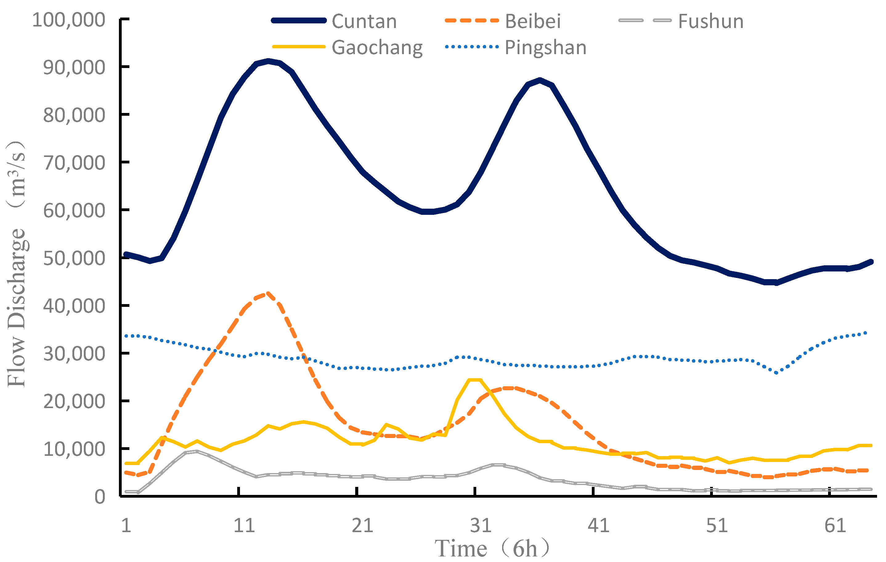
5. Results and Discussion

According to 1954 to 2020 synchronous observed flow data series of Pingshan, Gaochang, Fushun, Beibei, and Cuntan hydrologic stations, the flood regional composition characteristics of these hydrologic stations are shown in

Table 2. Flood regional composition characteristics of Cuntan hydrologic station.

River Name	Hydrologic Station	Catchment Area		W7d		W15d
		km2	%	108 m3	%	108 m3	%
Jinsha River	Pingshan	485,099	60.0	861	38.4	1730	41.6
Minjiang River	Gaochang	135,378	16.0	500	22.3	949	22.8
Tuo River	Fushun	74,248	4.2	319	5.4	282	6.8
Jialin River	Beibei	156,142	18.0	703	31.4	1070	25.7
Uncontrolled interval basin		15,692	1.8	57	2.5	129	3.1
Yangtze River	Cuntan	866,559	100	2240	100	4160	100

, in which the annual maximum 7-day (W_7d) and 15-day (W_15d) flood volumes at each hydrologic station and its proportion percentage of Cuntan station are also analyzed. For example, the catchment area of Jinsha River is 485,099 km², which accounts for 60% of Cuntan station, while the W_7d flood volume is 86.1 billion m³, which accounts for 38.4% of Cuntan station; the catchment area of Jialin River is 156,142 km², which accounts for 18.0% of Cuntan station, while the W_7d flood volume is 70.3 billion m³, which accounts for 31.4% of Cuntan station.

5.1. Flood Frequency Analysis at Cuntan Station

Cuntan hydrologic station began to observe water levels in 1892 and flow discharges in 1939. The flow discharge data series from 1892 to 1938 were interpolated and extended based on the rating curve of the water level and flow discharge relationship. The observed flow discharges from 1892 to 2022 and historical flood information in 1870 and 1788 were sampled to form a non-continuous annual maximum flood data series at Cuntan station. The plotting positions or empirical frequency F_Yt(y_t) for the flood data series is expressed by the following formula:

$$F_{Yt}(y_t)=\left\{\begin{array}{cc}{P}_M={\displaystyle \frac{M}{N+1}}\hfill & \hfill M=1,2,\dots ,a\\ P_m={\displaystyle \frac{1}{N+1}}\left[a+{\displaystyle \frac{N-a+1}{n-l+1}}(m-l)\right]\hfill & \hfill m=l+1,l+2,\dots ,a\end{array}\right.$$

(10)

where P_M and P_m are the empirical frequency of the Mth extraordinary floods and the mth observed floods, respectively; M represents the flood rank in the extraordinary flood sequence (M = 1, 2, …, a; a is the number of extraordinary floods); N denotes the length of the entire investigation period, which covers the historical information and observed floods; m denotes the flood rank in the observed flood sequence; n is the number of observed floods; and l represents the number of floods identified as extraordinary from the observed floods.

Pearson Type Three (P-III) distribution is one of the most popular distributions for fitting annual maximum flood magnitudes and has been recommended by the Ministry of Water Resources as a standard distribution for stationary flood frequency analysis in China [6]. Let stationary annual maximum flood data series X follow the P-III distribution with a density function $f(x)$ as follows:

$$f(x)={\displaystyle \frac{{\beta }^{\alpha }}{\mathrm{\Gamma }(\alpha )}}{(x-a_0)}^{\alpha -1}\exp [-\beta (x-a_0)]$$

(11)

where Γ(·) is the Gamma function; a₀, β, and α are the location, scale, and shape parameters of the P-III distribution, which could be estimated by the sample mean value (EX), coefficient of variation (Cv), and coefficient of skewness (Cs).

The P-III distribution coupled with the curve fitting method is recommended by the Ministry of Water Resources to estimate design floods in hydraulic engineering projects [6], where the sum of squared deviations (SSD) criterion is used to minimize the discrepancy between the empirical data points and the P-III distribution frequency curve.

Table 3. List of statistical and design flood values with different frequencies at Cuntian hydrologic station.

Flood	Statistical Values			Design Flood Values
	EX	CV	CS	0.01%	0.10%	1%	5%
Qm (m3/s)	51,600	0.25	0.75	121,000	105,000	88,700	75,200
W3d (108 m3)	124.0	0.25	0.625	282	248	210	180
W7d (108 m3)	244.0	0.22	0.55	509	452	390	340
W15d (108 m3)	450.0	0.210	0.525	911	814	705	618

lists the statistical and design flood values with different frequencies for peak discharge Q_m, W_3d, W_7d, and W_15d flood volumes at Cuntian hydrologic station, in which 100-year design peak discharge (Q_m), W_7d, and W_15d flood volumes are 88,700 m³/s, 390, and 705 10⁸ m³, respectively. The fitted P-III distribution frequency curves for Q_m, W_3d, W_7d, and W_15d at Cuntian station are also plotted in Figure 4. It is shown that the P-III distribution could fit the historical floods and annual maximum measured flood data series very well.

5.2. Design Flood Estimated by TYFC Method

Ten typical-year flood hydrographs were selected based on the characteristics of flood encounters of the Jinsha River, Min River, and Jialing River. The 7-day and 15-day flood volumes at each station are calculated and listed in

Table 4. Typical-year design flood regional composition at Cuntan hydrologic station.

Typical-Year	Flood Volume	Cuntan	Pingshan	Gaochang	Fushun	Beibei	Interval Basin
1961	W7d (108 m3)	261	31.0	88.0	27.0	111.0	4.0
	(%)	100	11.9	33.7	10.3	42.5	1.6
	W15d (108 m3)	470	91.0	164.0	42.0	163.0	10.0
	(%)	100	19.4	34.9	8.9	34.7	2.1
1966	W7d (108 m3)	336	152.0	91.0	14.0	58.0	21.0
	(%)	100	45.2	27.1	4.2	17.3	6.2
	W15d (108 m3)	581	302.0	141.0	22.0	89.0	27.0
	(%)	100	52.0	24.3	3.8	15.3	4.6
1981	W7d (108 m3)	331	89.0	60.0	33.0	137.0	12.0
	(%)	100	26.9	18.1	10.0	41.4	3.6
	W15d (108 m3)	535	167.0	121.0	45.0	175.0	27.0
	(%)	100	31.2	22.6	8.4	32.7	5.1
1982	W7d (108 m3)	213	83.0	40.0	4.0	80.0	6.0
	(%)	100	39.0	18.8	1.9	37.6	2.7
	W15d (108 m3)	399	164.0	75.0	8.0	129.0	23.0
	(%)	100	41.1	18.8	2.0	32.3	5.8
1989	W7d (108 m3)	249	66.0	43.0	5.0	122.0	13.0
	(%)	100	26.5	17.3	2.0	49.0	5.2
	W15d (108 m3)	419	135.0	89.0	10.0	160.0	25.0
	(%)	100	32.2	21.2	2.4	38.2	6.0
1991	W7d (108 m3)	269	109.0	69.0	16.0	43.0	32.0
	(%)	100	40.5	25.7	5.9	16.0	11.9
	W15d (108 m3)	480	227.0	132.0	22.0	58.0	41.0
	(%)	100	47.3	27.5	4.6	12.1	8.5
1998	W7d (108 m3)	296	115.0	57.0	20.0	91.0	13.0
	(%)	100	38.9	19.3	6.8	30.7	4.3
	W15d (108 m3)	545	242.0	97.0	30.0	132.0	44.0
	(%)	100	44.4	17.8	5.5	24.2	8.1
2010	W7d (108 m3)	257	71	43	7	108	28.0
	(%)	100	27.6	16.7	2.7	42.0	11.0
	W15d (108 m3)	500	138.0	97.0	19.0	208.0	38.0
	(%)	100	27.6	19.4	3.8	41.6	7.6
2012	W7d (108 m3)	275	99.0	70.0	20.0	47.0	39.0
	(%)	100	36.0	25.5	7.3	17.1	14.1
	W15d (108 m3)	507	201.0	127.0	27.0	76.0	76.0
	(%)	100	39.6	25.0	5.3	15.0	15.1
2020	W7d (108 m3)	390	81.0	115.0	32.0	158.0	4.0
	(%)	100	20.8	29.5	8.2	40.5	1.0
	W15d (108 m3)	642	161.0	174.0	52.0	226.0	29.0
	(%)	100	25.1	27.1	8.1	35.2	4.5

, where the proportion percentage of flood volume at each station to Cuntan station are also given. For example, in the 1961 typical-year, the 7-day flood volumes (W_7d) at Pingshan, Gaochang, Fushun, Beibei, and interval basin are 3.1, 8.8, 2.7, 11.1, and 0.4 billion m³, which account for 11.9%, 33.7%, 10.3%, 42.5%, and 1.6% of that at Cuntan station. While in 2020 typical-year, the 15-day flood volumes (W_15d) at Pingshan, Gaochang, Fushun, Beibei, and interval basin are 161, 174, 52, 226, and 29 10⁸ m³, which account for 25.1%, 27.1%, 8.1%, 35.2%, and 4.5% of that at Cuntan station.

Figure 5 shows the observed flood hydrographs in the 1998 typical-year at the Pingshan, Gaochang, Fushun, Beibei, and Cuntan hydrologic stations. It shows that double flood peaks occurred at Cuntan hydrologic station, which mainly came from the Jialin River observed at Beibei station.

5.3. Design Flood Estimated by FRC-POD Method

The annual maximum flood volume data series at upstream hydrologic stations corresponding to the occurrence date of the annual maximum flood volume at design site are sampled to form the regional flood volume set. The singular value decomposition is carried out to obtain the main paradigm of the regional W_7d and W_15d flood volumes. Figure 6 plots the energy contribution rate of each paradigm for regional W_7d and W_15d flood volumes, Figure 7 is the first normal values of W_7d and W_15d flood volumes, and Figure 8 shows the first paradigm coefficient values of each site for regional W_7d and W_15d flood volumes.

The main paradigms that contributed more than 30% of the annual maximum flood volume are selected, and the flood regional compositions are reconstructed through Equation (9). As can be seen in Figure 6, the first two paradigms of the regional flood volume contribute more than 30% of the annual maximum flood volume, and thus the paradigm coefficients T₁ and T₂ are selected. The reconstruction results are scaled by the same ratio based on the design flood volumes to obtain the design flood regional composition for the study region.

5.4. Design Flood Estimated by MLFRC Method

Compared to Archimedean copula and t-copula, vine-copula functions are more flexible and practical in describing the correlation of variables, especially for describing characteristics such as inconsistent and asymmetric correlation structures between two variables. Zhong et al. [25] introduced vine-copula into MLFRC framework to estimate design flood of cascade reservoirs and showed that the vine-copula is much better than t-copula in a high-dimension cascade reservoir system.

According to the various connection structures among pair copulas, vine-copula is classified into the three categories as C-vine-copula, D-vine-copula, and R-vine-copula. C-vine-copula and D-vine-copula are commonly used in hydrological analysis, which can be expressed by the following equations, respectively:

$$f(x_1,x_2,\dots ,x_n)={\displaystyle \prod _{k=1}^{n}f(x_k)}{\displaystyle \prod _{j=1}^{n-1}{\displaystyle \prod _{i=1}^{n-j}{c}_{j,i+j|1,\dots ,j-1}(F(x_j | x_1,\dots ,x_{j-1}),F(x_{i+j} | x_1,\dots ,x_{j-1}))}}$$

(12)

$$f(x_1,x_2,\dots ,x_n)={\displaystyle \prod _{k=1}^{n}f(x_k)}{\displaystyle \prod _{j=1}^{n-1}{\displaystyle \prod _{i=1}^{n-j}{c}_{j,i+j|i+1,\dots ,i+j-1}(F(x_i | x_{i+1},\dots ,x_{i+j-1}),F(x_{i+j} | x_{i+1},\dots ,x_{i+j-1}))}}$$

(13)

Therefore, the vine-copula-based MLFRC method was used to establish the joint distribution of the annual maximum W_7d and W_15d flood volume for each sub-basin in the upper part of Cuntan station. The theoretical joint frequency F_T is calculated with the integral of Equations (12) and (13), while the empirical frequency F_E is calculated by the following:

$$F_E(i)=i/(m+1)$$

(14)

where i is the sample rank in ascending order, and m is the total number of years.

The P-P plot of the empirical and theoretical joint distribution obtained by fitting the vine-copula function is shown in Figure 9.

It can be seen from Figure 9 that the points are basically located near the line, which indicates that it can simulate the joint distribution of the annual maximum flood volumes very well in the upper Cuntan station.

After constructing the joint distribution of floods in each sub-basin, the MLFRC at Cuntan station can be deduced. The most likely regional flood compositions with different design frequencies at Cuntan hydrologic station are shown in

Table 5. Design flood volumes with different frequencies estimated by MLFRC method at Cuntan hydrologic station (10⁸ m³).

Design Frequency		0.1%	0.50%	1%	2%	5%	10%	20%
Cuntan station	W7d	452	410	390	369	340	315	287
	W15d	814	740	705	670	618	575	526
Pingshan station	W7d	116	113	111	108	104	98.8	94.3
	W15d	243	221	242	215	199	192	174
Gaochang station	W7d	123	114	100	96.9	82.6	72.9	63.0
	W15d	181	158	156	152	138	126	118
Fushun station	W7d	1.96	3.22	7.42	7.37	10.9	15.9	18.5
	W15d	24.1	29.6	23.2	27.3	34.2	38.9	40.2
Beibei station	W7d	136	126	125	115	106	103	94
	W15d	239	222	196	192	183	175	151
Interval basin	W7d	76.1	53.2	47.1	41.4	36.8	24.9	17.0
	W15d	126	110	88.4	83.1	64.5	43.3	42.9

. For example, the 1000-year design W_15d flood volumes at Pingshan, Gaochang, Fushun, Beibei, and Cuntan hydrologic stations are 243, 181, 24.1, 239, and 814 10⁸ m³, respectively.

5.5. Comparative Study

5.5.1. Flood Regional Compositions at Cuntan Station

The typical-year flood composition (TYFC) method is simple and has been widely applied to estimate design flood in China. However, the TYFC method depends on the selected typical-year flood, which is a subjective judgment. The proposed FRC-POD method can consider all typical-year flood regional compositions and the multi-site flood source characteristics, which has more statistical rationality than the TYFC method.

Further comparison among the proposed FRC-POD method, the TYFC method, and the MLFRC method is carried out as follows:

Taking the 100-year design W_15d as an example, the differences in the flood regional composition at Cuntan station were estimated by the three FRC methods.

Table 6. Comparison of flood proportions estimated by FRC methods for multi-site flood sources.

Methods		Cuntan	Pingshan	Gaochang	Fushun	Beibei	Interval Basin
FRC-POD method		100	40	21	2	20	17
MLFRC method		100	30	21	4	30	15
TYFC method	1966	100	52	24	4	15	5
	1981	100	31	23	8	33	5
	1998	100	44	18	6	24	8
	2012	100	40	25	5	15	15
	2020	100	25	27	8	35	5

compares the flood proportions estimated by the FRC methods for multi-site flood sources. Figure 10 shows the flood proportions estimated by different FRC methods for multi-site flood sources. The 1966, 1998, and 2012 typical-years with large floods occurred in Jinsha River basin; the flood regional composition results at Cuntan Station estimated by these FRC methods are similar, with the flood proportion of W_15d at Pingshan station ranging from 44% to 52% of that at Cuntan station. Similar flood proportions of W_15d at Gaochang, Fushun, and Beibei stations range from 14% to 25%, 2% to 6%, and 15% to 29% of that at Cuntan station. In the years 1981 and 2020 with large floods occurring in the Jialing River, the flood proportions estimated by the MLFRC and FRC-POD methods are different from that of the TYFC method.

Pingshan station is the outlet of the Jinsha River basin and its flood is regulated by the upstream cascade reservoirs. The proposed FRC-POD method, which takes into account the multi-site flood source characteristics, can identify Pingshan station as one of the major flood sources. Compared with the TYFC and the MLFRC methods, the FRC-POD method can also recognize the possibility of major floods coming from the uncontrolled interval basin, which is more detrimental for flood control when a major flood occurs in the uncontrolled inter-basin. Therefore, the FRC-POD method is more reasonable based on statistical theory, which meanwhile highlights the practical significance of the mainstream and uncontrolled inter-basin floods for downstream flood prevention.

The rationality of different FRC methods is also analyzed through the observed flood data series. The flow routing time from Pingshan station of Jinsha River to Beibei station of Jialin River is about 31 h. The annual maximum flood occurrence times and flood volumes at Pingshan and Beibei stations in 1951~2022 considering the flood routing propagation time are shown in

Table 7. Statistics of flood volume encounters between Pingshan and Beibei stations.

Flood Volume	Year	Pingshan Station			Beibei Station			η
		Start Date	W	RP	Start Date	W	RP
W7d (108 m3)	1959	12 August	79.0	<5	11 August	48.4	<5	1.63
	1966	29 August	163.1	30	30 August	59.1	<5	2.76
	1983	1 August	61.4	<5	31 July	107.5	5~10	0.57
	1992	13 July	59.7	<5	14 July	98.6	<5	0.61
W15d (108 m3)	1953	24 July	147.2	<5	24 July	107.1	<5	1.37
	1959	5 August	145.7	<5	10 August	78.9	<5	1.85
	1962	10 August	246.8	5~10	16 August	125.2	<5	1.97
	1964	11 September	176.2	<5	10 September	168.2	5~10	1.05
	1971	15 August	142.5	<5	13 August	64.5	<5	2.21
	1982	20 July	166.3	<5	17 July	153.1	<5	1.09
	1984	9 July	159.8	<5	3 July	173.0	5~10	0.92
	1992	8 July	121.2	<5	14 July	127.7	<5	0.95
	1996	22 July	175.7	<5	22 July	44.6	<5	3.94
	1997	9 July	190.2	<5	3 July	47.3	<5	4.02
	2004	3 September	180.4	<5	29 August	110.0	<5	1.64
	2006	7 July	113.0	<5	1 July	45.9	<5	2.46
	2009	6 August	180.7	<5	1 August	96.1	<5	1.88

Note: W—flood value; RP—return period; η—ratio of flood volume between Pingshan Station and Beibei station.

. It can be seen that when the floods of Jinsha River and Jialing River encounter, the flood volume of Jinsha River is 0.56~4.02 times of flood volume of Jialing River. The ratios of the flood volume of Jinsha River and Jialin River calculated by the FRC-POD and MLFRC methods are about 2 and 1, respectively, which are similar to 1959, 1963, and 1971 typical-year floods.

The annual maximum flood occurrence times and flood volume of Gaochang and Beibei stations in 1951~2022 considering the flood routing time are also shown in

Table 8. Statistics of flood encounters between Gaochang and Beibei stations.

Flood Volume	Year	Gaochang Station			Beibei Station			δ
		Start Date	W	RP	Start Date	W	RP
W7d (108 m3)	1957	14 July	54.29	<5	14 July	90.55	<5	0.60
	1959	10 August	89.19	10~20	11 August	48.41	<5	1.84
	1961	26 June	87.64	10~20	27 June	111.11	5~10	0.79
	1964	10 September	71.28	<5	Sept. 10	90.20	<5	0.79
	1966	30 August	96.60	20~30	30 August	59.14	<5	1.63
	1977	7 July	54.67	<5	7 July	84.74	<5	0.65
	1981	10 July	78.26	5~10	13 July	138.68	<5	0.56
	1997	4 July	48.50	<5	3 July	30.62	<5	1.58
	2003	28 August	61.37	<5	30 August	86.29	<5	0.71
	2006	5 July	32.50	<5	3 July	32.27	<5	1.01
	2009	31 July	45.18	<5	2 August	76.12	<5	0.59
	2018	12 July	75.40	5~10	11 July	116.73	10~20	0.65
	2020	13 August	110.6	10~20	14 August	155	50	0.71
W15d (108 m3)	1953	19 July	98.17	<5	24 July	107.11	<5	0.92
	1957	8 July	101.85	<5	7 July	144.91	<5	0.70
	1958	10 August	141.32	5~10	13 August	156.25	<5	0.90
	1961	26 June	162.71	10~20	25 June	163.79	5~10	0.99
	1964	9 September	126.49	<5	10 September	168.19	5~10	0.75
	1965	9 July	119.70	<5	9 July	158.66	<5	0.75
	1970	28 July	99.67	<5	28 July	70.78	<5	1.41
	1971	10 August	89.02	<5	13 August	64.51	<5	1.38
	1977	2 July	91.32	<5	7 July	110.45	<5	0.83
	1995	12 August	104.87	<5	12 August	65.15	<5	1.61
	1996	20 July	98.45	<5	22 July	44.58	<5	2.21
	1997	28 June	85.54	<5	3 July	47.30	<5	1.81
	2003	26 August	109.07	<5	29 August	138.01	<5	0.79
	2006	5 July	64.40	<5	1 July	45.93	<5	1.40
	2010	13 July	98.04	<5	16 July	207.08	50	0.47
	2013	5 July	114.28	<5	10 July	178.54	10	0.64
	2018	8 July	138.97	5~10	3 July	199.51	20	0.70
	2020	11 August	176.5	10~20	12 August	223.8	20	0.79

Note: δ—the ratio of flood volume between Gaochang station and Beibei station.

. It can be seen that when the flood is between Min River and Jialin River, the flood volume of Min River is 0.47~2.21 times the flood volume of Jialing River. The ratios of the flood volume of Min River and Jialin River calculated by the FRC-POD and MLFRC methods are 1.05 and 0.7, respectively. The ratio of the FRC-POD method is similar to 1953, 1958, 1961, and 2006 typical-years. The ratio of the MLFRC method is similar to 1981 and 2020 typical-years. This reflects that the FRC-POD method and MLFRC method are rational and representative.

5.5.2. Design Flood Estimation at Cuntan Station

Based on the flood regional composition of Cuntan Station calculated by the FRC-POD, MLFRC, and TYFC (selceting 1998 typical-year) methods, the design floods at Cuntan station are estimated and shown in

Table 9. Comparison of 1000-year design floods estimated by three RFC methods at Cuntan hydrologic station.

Probability	Design Flood	Original Value	FRC-POD	MLFRC	TYFC-1998
0.10%	Qm (m3/s)	105,000	61,600 (−41.3%)	65,400 (−37.8%)	56,500 (−46.2%)
	W3d 108 m3)	248	148 (−40.2%)	161 (−35.2%)	136 (−45.0%)
	W7d (108 m3)	452	287 (−36.6%)	315 (−30.4%)	265 (−41.4%)
	W15d (108 m3)	814	532 (−34.7%)	592 (−27.3%)	500 (−38.6%)
1%	Qm (m3/s)	88,700	48,300 (−45.6%)	50,000 (−43.6%)	44,700 (−49.6%)
	W3d 108 m3)	210	117 (−44.3%)	122 (−42.1%)	109 (−48.1%)
	W7d (108 m3)	390	248 (−36.5%)	261 (−33.1%)	235 (−39.8%)
	W15d (108 m3)	705	473 (−33.0%)	506 (−28.3%)	449 (−36.3%)
2%	Qm (m3/s)	82,900	46,500 (−44.0%)	49,400 (−40.5%)	42,900 (−48.2%)
	W3d 108 m3)	198	112 (−43.3%)	120 (−39.2%)	105 (−47.0%)
	W7d (108 m3)	369	237 (−35.8%)	258 (−30.3%)	225 (−39.1%)
	W15d (108 m3)	670	453 (−32.4%)	499 (−25.5%)	429 (−36.0%)
5%	Qm (m3/s)	75,200	43,300 (−42.4%)	(−38.7%)	40,500 (−46.1%)
	W3d 108 m3)	180	105 (−41.9%)	112 (−37.6%)	98.8 (−45.1%)
	W7d (108 m3)	340	222 (−34.8%)	(−28.9%)	210 (−38.3%)
	W15d (108 m3)	618	424 (−31.4%)	469 (−24.1%)	400 (−35.3%)

. After considering the regulation of upstream 22 large-scale reservoirs and comparing them with the originally designed values, the 1000-year design peak discharge and 3d, 7d, and 15d flood volumes estimated by the proposed FRC-POD method are decreased by 41.3%, 40.2%, 36.6%, and 34.7%, respectively.

The 1000-year and 100-year design flood hydrographs at Cuntan station derived by three different FRC methods are plotted in Figure 11. It is shown that the shapes of these flood hydrographs are similar, and the estimated results of the FRC-POD method are between those of the MLFRC and TYFC-1998 methods.

6. Conclusions

The regulation of upstream cascade reservoirs has significantly altered the downstream hydrologic regime and reduced the peak discharge and flood volumes. In this study, a novel flood regional composition method considering typical-year and multi-site flood source characteristics was proposed to estimate design floods at the Cuntan hydrologic station in the upper Yangtze River. The comparative study clarified its practicality and rationality. The main conclusions are summarized as follows:

(1) In the typical-years of 1966, 1998, and 2012 with large floods occurring in the Jinsha River, the design floods at Cuntan station estimated by the three FRC methods are basically the same. The proportion of 15d flood volume at Pingshan station ranges from 44% to 52% of that at Cuntan station, and the proportion of 15d flood volume at Gaochang station is ranges from 14% to 25% of that at Cuntan station.

(2) The rationality of different flood regional composition methods is verified through flood encounter analysis between Pingshan (or Gaochang) and Beibei stations, which shows that the flood regional composition computed by the proposed FRC-POD and MLFRC methods are rational and representative.

(3) Compared with the originally designed flood values based on natural annual maximum flow data series, the 1000-year design peak discharge, 3 d, 7 d, and 15 d flood volumes estimated by the FRC-POD method are decreased by 41.3%, 40.2%, 36.6%, and 34.7%, respectively, after considering the regulation impact of the upper 22 large-scale reservoirs.

(4) The proposed FRC-POD method and the current EFRC and MLFRC methods obtained similar design flood estimation results in the upper Yangtze River basin. However, the current EFRC and MLFRC methods depend on selected typical-year flood events to amplify the design flood hydrograph, which has many results, while the proposed FRC-POD method has only one final solution, which is more reasonable in practical application.

The limitation of the FRC-POD method is that it needs the amount of flow data observed by many hydrologic stations simultaneously, which may limit its application.

References

1. Guo, S.; Zhang, H.; Chen, H.; Peng, D.; Liu, P.; Pang, B. A reservoir flood forecasting and control system for China. Hydrol. Sci. J. 2004, 49, 959–972. [Google Scholar] [CrossRef]
2. Duan, W.; Guo, S.; Wang, J.; Liu, D. Impact of cascaded reservoirs group on flow regime in the middle and lower reaches of the Yangtze River. Water 2016, 8, 218. [Google Scholar] [CrossRef]
3. Guo, S.; Muhammad, R.; Liu, Z.; Xiong, F.; Yin, J. Design flood estimation methods for cascade reservoirs based on copulas. Water 2018, 10, 560. [Google Scholar] [CrossRef]
4. Yue, S.; Ouarda, T.B.; Bobée, B.; Legendre, P.; Bruneau, P. Approach for describing statistical properties of flood hydrograph. J. Hydrol. Eng. 2002, 7, 147–153. [Google Scholar]
5. Xiao, Y.; Guo, S.L.; Chen, L. Design flood hydrograph based on multi-characteristic synthesis index method. J. Hydrol. Eng. 2009, 14, 1359–1364. [Google Scholar]
6. MWR (Ministry of Water Resources). Regulation for Calculating Design Flood of Water Resources and Hydropower Projects; Water Resources and Hydropower Press: Beijing, China, 2006. (In Chinese) [Google Scholar]
7. Xiong, F.; Guo, S.; Liu, P.; Xu, C.-Y.; Zhong, Y.; Yin, J.; He, S. A general framework of design flood estimation for cascade reservoirs in operation period. J. Hydrol. 2019, 577, 124003. [Google Scholar]
8. Xiong, F.; Guo, S.; Yin, J.; Tian, J.; Rizwan, M. Comparative study of flood regional composition methods for design flood estimation in cascade reservoir system. J. Hydrol. 2020, 590, 125530. [Google Scholar]
9. De Michele, C.; Salvadori, G. A generalized pareto intensity-duration model of storm rainfall exploiting 2-Copulas. J. Geophys. Res. 2003, 108. [Google Scholar] [CrossRef]
10. Salvadori, G.; Michele, C. Frequency analysis via copulas: Theoretical aspects and applications to hydrological events. Water Resour. Res. 2004, 40, W125111. [Google Scholar]
11. Poulin, A.; Huard, D.; Favre, A.C.; Pugin, S. Importance of tail dependence in bivariate frequency analysis. J. Hydrol. Eng. 2007, 12, 394–403. [Google Scholar]
12. Arnaud, P.; Cantet, P.; Odry, J. Uncertainties of flood frequency estimation approaches based on continuous simulation using data resampling. J. Hydrol. 2017, 554, 360–369. [Google Scholar] [CrossRef]
13. Yin, J.; Guo, S.; Liu, Z.; Yang, G.; Zhong, Y.; Liu, D. Uncertainty analysis of bivariate design flood estimation and its impacts on reservoir routing. Water Resour. Manag. 2018, 32, 1795–1809. [Google Scholar] [CrossRef]
14. Nelsen, R.B. An Introduction to Copulas, 2nd ed.; Springer: New York, NY, USA, 2006. [Google Scholar]
15. Salvadori, G.; Durante, F.; Michele, C.; Bernardi, M.; Petrella, L. A multivariate copula-based framework for dealing with hazard scenarios and failure probabilities. Water Resour. Res. 2016, 52, 3701–3721. [Google Scholar] [CrossRef]
16. Karhunen, K. Zur spektral theorie stochasticher prozesse. Ann. Acad. Sci. Fenn. 1946, 34, 1–7. [Google Scholar]
17. Aubry, N. On the hidden beauty of the proper orthogonal decomposition. Theor. Comput. Fluid Dyn. 1991, 2, 339–352. [Google Scholar] [CrossRef]
18. Higham, J.E.; Brevis, W.; Keylock, C.J.; Safarzadeh, A. Using modal decompositions to explain the sudden expansion of the mixing layer in the wake of a groyne in a shallow flow. Adv. Water Resour. 2017, 107, 451–459. [Google Scholar] [CrossRef]
19. Kutz, N.J.; Brunton, S.L.; Brunton, B.W.; Proctor, J.L. Dynamic Mode Decomposition: Data-Driven Modeling of Complex Systems; Society for Industrial and Applied Mathematics: Philadelphia, PA, USA, 2016. [Google Scholar]
20. Higham, J.E.; Brevis, W.; Keylock, C.J. Implications of the selection of a particular modal decomposition technique for the analysis of shallow flows. J. Hydraul. Res. 2018, 56, 796–805. [Google Scholar] [CrossRef]
21. Feeny, B.F.; Liang, Y. Interpreting proper orthogonal modes of randomly excited vibration systems. J. Sound Vib. 2003, 265, 953–966. [Google Scholar] [CrossRef]
22. Jiang, C.; Xiong, L.; Xu, C.; Yan, L. A river network-based hierarchical model for deriving flood frequency distributions and its application to the upper Yangtze basin. Water Resour. Res. 2021, 57, 029374. [Google Scholar] [CrossRef]
23. Nguyen-Tien, V.; Elliott, R.; Strobl, E.A. Hydropower generation, flood control and dam cascades: A national assessment for Vietnam. J. Hydrol. 2018, 560, 109–126. [Google Scholar] [CrossRef]
24. Li, T.; Guo, S.; Chen, L.; Guo, J. Bivariate flood frequency analysis with historical information based on Copula. J. Hydrol. Eng. 2013, 18, 1018–1030. [Google Scholar] [CrossRef]
25. Zhong, S.; He, Y.; Guo, S.; Xie, Y.; Xu, C.-Y. Design flood estimation of cascade reservoirs based on vine-copula flood regional composition. J. Hydrol. Reg. Stud. 2024, 56, 102071. [Google Scholar]
Figure 1. Sketch diagram of cascade reservoir in river basin.
Water 17 01106 g001
Figure 2. Flow chart of proposed FRC-POD method.
Water 17 01106 g002
Figure 3. Sketch map of upper Yangtze River and investigated hydrologic stations and reservoirs.
Water 17 01106 g003
Figure 4. The fitted P-III distribution flood frequency curves at Cuntian hydrologic station.
Water 17 01106 g004
Figure 5. Observed flood hydrographs in 1998 typical-year at Pingshan, Gaochang, Fushun, Beibei, and Cuntan hydrologic stations.
Water 17 01106 g005
Figure 6. Energy contribution rate of each paradigm for regional W7d and W15d flood volumes.
Water 17 01106 g006
Figure 7. First normal values of W7d and W15d flood volumes.
Water 17 01106 g007
Figure 8. First paradigm coefficient values of W7d and W15d flood volumes.
Water 17 01106 g008
Figure 9. Scatters of empirical frequency and theoretical frequency of annual maximum W7d and W15d flood volume data series fitted by vine-copula.
Water 17 01106 g009
Figure 10. Flood proportions estimated by different FRC methods for multi-site flood sources.
Water 17 01106 g010
Figure 11. Comparison of design flood hydrographs derived from different methods at Cuntan station.
Water 17 01106 g011