Evaluation of ICESat-2 Laser Altimetry for Inland Water Level Monitoring: A Case Study of Canadian Lakes

Abstract

This study evaluates the performance of the ICESat-2 ATL13 altimetry product for estimating water levels in 182 Canadian lakes by integrating satellite-derived observations with in situ gauge measurements and applying spatial filtering using the HydroLAKES dataset. The analysis compares ATL13-derived lake surface elevations with hydrometric data from national monitoring stations, providing a robust framework for assessing measurement accuracy. Statistical metrics—including root mean square error (RMSE), mean absolute error (MAE), and mean bias error (MBE)—are employed to quantify discrepancies between the datasets. Importantly, the application of HydroLAKES-based filtering reduces the mean RMSE from 1.53 m to 1.40 m, and the further exclusion of high-error lakes lowers it to 0.96 m. Larger and deeper lakes exhibit lower error margins, while smaller lakes with complex shorelines show greater variability. Regression analysis confirms the excellent agreement between satellite and gauge measurements (R² = 0.9999; Pearson’s r = 0.9999, n = 182 lakes, p < 0.0001). Temporal trends reveal declining water levels in 134 lakes and increasing levels in 48 lakes from 2018 to 2024, potentially reflecting climatic variability and human influence. These findings highlight the potential utility of ICESat-2 ATL13 altimetry for large-scale inland water monitoring when combined with spatial filtering techniques such as HydroLAKES.

1. Introduction

Monitoring inland water levels with precision is essential for understanding hydrological processes, managing freshwater resources, and assessing the impacts of climate change on aquatic systems [1]. Lakes play a critical role in regulating the hydrological cycle [2], influencing regional climate patterns [3], and supporting diverse ecological communities [4]. For instance, lakes can modulate local climate conditions by acting as carbon sinks and altering greenhouse gas fluxes in their surrounding environments [5]. Moreover, they are vital for various human needs, including agriculture, hydroelectric power generation, and drinking water supply. However, lake and river water levels vary significantly across space and time due to precipitation, evaporation, groundwater interactions, and anthropogenic factors such as dam operations and water extraction [6]. Understanding these dynamics is crucial for reducing environmental risks and enabling sustainable water management. As climate variability intensifies, the demand for accurate, continuous, and spatially extensive water level data have increased, revealing the inherent limitations of traditional hydrological monitoring methods [7].

Traditionally, water levels have been monitored using in situ gauge stations, which provide long-term, high-frequency, and high-accuracy measurements at specific locations. These ground-based observations are invaluable, because they enable detailed analyses of local hydrological dynamics, support water resource planning, and serve as reference data for calibrating remote sensing methods. However, despite their precision, the spatial coverage of gauge networks is inherently limited [8]. Most stations are located in accessible or economically prioritized regions, often near urban centers or major infrastructure. In contrast, large areas—particularly those in remote, high-latitude, or sparsely populated regions—remain under-monitored due to the logistical, financial, and technical challenges associated with deploying and maintaining monitoring infrastructure. As a result, significant data gaps persist, constraining our ability to model hydrological processes at broad scales and to respond effectively to environmental changes [9]. These limitations have spurred interest in alternative measurement approaches, particularly satellite-based methods capable of providing consistent, wide-area water level observations [10].

In recent decades, satellite altimetry has transformed hydrological monitoring by offering extensive spatial coverage and enabling the observation of inland water bodies at a global scale. Unlike traditional gauge stations, satellite-based measurements are not constrained by physical accessibility and can provide consistent water level data across remote and hard-to-reach regions [11]. Early radar altimetry missions, such as TOPEX/Poseidon, Jason-1/2/3, and ENVISAT, demonstrated the feasibility of retrieving inland water levels by measuring the time delay of radar pulses reflected from water surfaces [12,13,14]. However, since these missions were primarily optimized for open-ocean observations, their coarse spatial resolution limited their effectiveness in monitoring smaller lakes and rivers [15]. A significant advancement in inland water monitoring came with the launch of NASA’s Ice, Cloud, and Land Elevation Satellite (ICESat) in 2003 [16]. As the first spaceborne lidar altimeter dedicated to precise elevation measurements, ICESat provided valuable insights into ice sheet dynamics, land topography, and freshwater systems [17]. Despite its utility, the mission’s single-beam laser system and intermittent acquisition schedule limited its spatial and temporal coverage [18,19]. This limitation was addressed with the launch of ICESat-2 in 2018, which marked a major technological leap in satellite altimetry [20]. Equipped with the Advanced Topographic Laser Altimeter System (ATLAS), ICESat-2 utilizes a photon-counting lidar system capable of delivering sub-decimeter vertical accuracy [21]. By employing six laser beams instead of one, ICESat-2 significantly enhances both data density and spatial coverage, making it suitable for monitoring narrow, fragmented, or seasonally dynamic inland water bodies [13]. These improvements have unlocked new possibilities for capturing water level changes at fine spatial and temporal scales, advancing our understanding of hydrological variability and climate-driven transformations in freshwater environments [22,23,24].

While ICESat-2 represents a major advancement in satellite altimetry, several challenges remain regarding the reliability and applicability of its ATL13 data product for estimating water levels. Although its high-resolution laser altimetry offers significant improvements over traditional radar-based techniques, a variety of environmental factors can still affect the accuracy of measurements [25]. Ice cover, surface wave activity, vegetation interference, and atmospheric conditions can introduce uncertainties in water surface detection, thereby limiting the precision of ATL13-derived elevations [26,27,28,29]. Furthermore, while larger lakes benefit from stronger signal returns and higher beam densities, smaller lakes—particularly those with irregular shorelines or dynamic water levels—pose greater challenges for accurate retrieval [30]. These issues underscore the importance of validating ICESat-2-derived water level estimates against in situ gauge observations. Ensuring the reliability of satellite altimetry for hydrological applications requires a thorough assessment of measurement uncertainty and systematic comparison with ground-based data to refine processing techniques and improve overall accuracy.

To address these challenges and improve the accuracy of satellite-based water level monitoring, integrating high-resolution geospatial datasets has become essential. In this study, I utilize the HydroLAKES database, which provides detailed shoreline polygons for more than 1.4 million lakes globally [31]. By accurately delineating lake boundaries, HydroLAKES enables the spatial filtering of ATL13 measurements, thereby reducing contamination from adjacent land surfaces and ensuring that only valid water surface returns are retained. This step is particularly critical when ICESat-2′s laser footprints intersect non-water areas, such as shorelines or nearby terrain, which can introduce significant errors into water level estimates. By enhancing the spatial attribution of ICESat-2 data, HydroLAKES improves the reliability of satellite-derived measurements and supports a more precise characterization of hydrological variability. This integration is especially beneficial for small or irregularly shaped lakes, where boundary precision plays a key role in minimizing measurement uncertainty. Since this study includes a substantial number of such lakes, accurate boundary delineation is crucial for producing reliable water level estimates and reducing retrieval errors in complex monitoring environments.

While satellite altimetry has significantly advanced hydrological monitoring, critical research gaps remain, especially in diverse and under-observed aquatic environments. Previous studies have primarily focused on large, well-instrumented water bodies, where in situ gauge networks enable the direct validation of satellite-derived measurements [32,33]. For example, Braun et al. [34] used ICESat (GLAS) data to monitor water levels in the Great Lakes and validated their results against radar altimetry and tide gauge data. Similarly, Xiang et al. [35] compared three satellite laser altimetry missions (ICESat-1, ICESat-2, and GEDI) for evaluating water levels in the Great Lakes and the Mississippi River system. However, many lakes in remote or high-latitude regions still lack dense monitoring networks, limiting validation opportunities. Balsamo et al. [36] and Du et al. [37] emphasized that satellite remote sensing is crucial for these data-sparse regions, although challenges remain in addressing seasonal and spatial variability. This issue is particularly prominent in Canada, which contains over two million lakes across a wide range of ecological zones—from glacially fed alpine lakes in British Columbia to boreal and subarctic systems in the Prairie Provinces and northern territories. Erler [38] highlighted hydro-climatic variability in the Fraser and Athabasca River basins, while Curran and Biles [39] demonstrated the hydrological complexity of northern water bodies such as those in the Brooks Range and the glacier-fed basins along the Gulf of Alaska.

To address this gap, my study provides the first comprehensive assessment of ICESat-2 ATL13 data across 182 Canadian lakes of varying sizes, shapes, elevations, and climates. Unlike previous research which was limited to larger lakes with robust gauge coverage, this analysis incorporates a diverse and geographically distributed sample, including many smaller and under-monitored lakes. By combining satellite altimetry with HydroLAKES spatial filtering and in situ gauge comparisons, I evaluate how lake morphology and regional factors influence measurement accuracy. This study contributes new insights into the conditions under which ICESat-2 performs reliably and highlights its potential to extend hydrological monitoring to remote regions where traditional methods fall short.

2. Materials and Methods

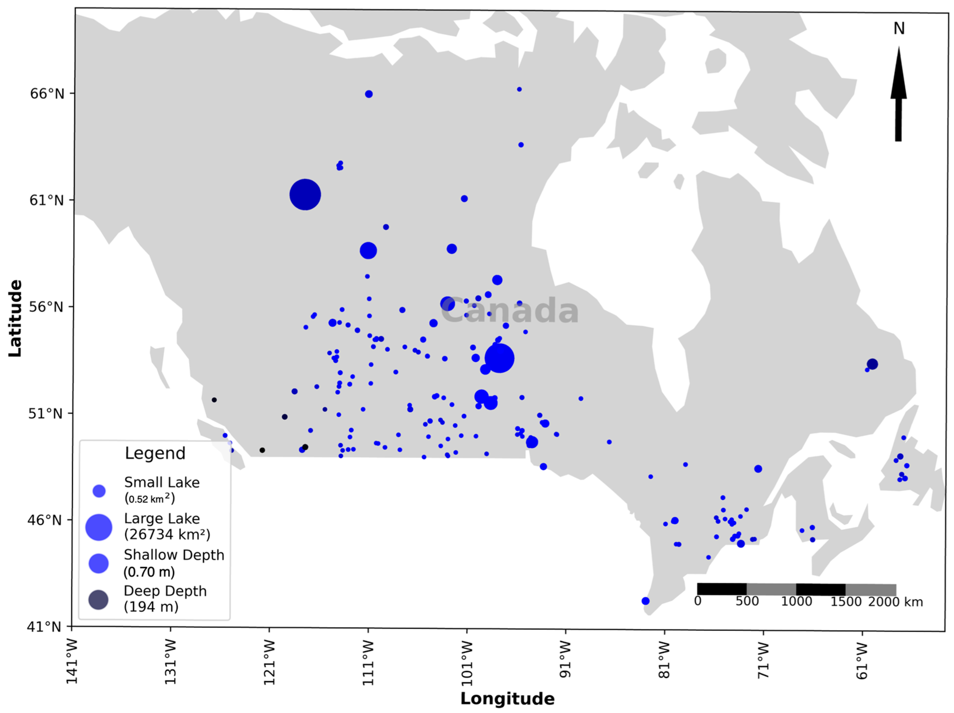
2.1. Geographical Scope of the Study

The study encompasses 182 lakes distributed across Canada, representing a diverse array of hydrological, ecological, and morphological characteristics. These lakes are situated across multiple climatic zones, ranging from boreal environments in the north to temperate regions in the south, thereby offering a robust basis for evaluating the performance of ICESat-2 ATL13 altimetry data. As shown in Figure 1, the dataset includes lakes with a wide range of surface areas, depths, and elevations. For example, Great Slave Lake is one of the largest and deepest, with a surface area of 26,734 km² and a maximum depth of 59 m [40]; Lake Winnipeg also has a large surface area (23,923 km²) but is comparatively shallow, with a depth of 11.9 m [41]. Harrison Lake stands out due to its depth, reaching 194 m [42], while Lake Minnewanka is located at a high elevation of 1469 m above sea level [43]. This variability illustrates the geographical and morphological diversity of the lakes in the dataset, enabling a comprehensive analysis of satellite altimetry performance across a range of inland water conditions.

Figure 2 depicts the relationship between lake elevation and average depth, revealing a more widespread elevation distribution rather than isolated outliers. While most lakes cluster at lower elevations with shallow depths, exceptions like Harrison Lake (red square in Figure 2) for its depth and Lake Minnewanka (green square in Figure 2) for its elevation illustrate the dataset’s range and variability. To ensure that this variability is systematically captured, the selection of lakes in this study is guided by multiple criteria aimed at maximizing environmental and geographical diversity. The dataset includes lakes with a broad spectrum of depths, elevations, and surface areas, distributed across different climatic zones throughout Canada. Lakes with significant surface areas are prioritized for robust altimetry performance, while the availability of long-term gauge and water level data enables meaningful trend analysis. This approach leads to a representative sample of 182 lakes, including large and ecologically significant systems such as Great Slave Lake—one of Canada’s deepest and most voluminous lakes—and Lake Winnipeg, a key basin with known hydrological variability. Meanwhile, lakes such as Harrison Lake (noted for its exceptional depth) and Lake Minnewanka (located at a high elevation) are included as distinctive edge cases to evaluate ICESat-2’s performance under challenging physical conditions. Together, this combination of representative, extreme, and widely distributed lake types provides a robust foundation for assessing inland water level retrieval across Canada’s diverse hydro-ecological regions.

2.2. Data

2.2.1. ICESat-2 ATL13

In this study, the ICESat-2 ATL13 dataset—specifically designed for inland water level monitoring—was utilized. ICESat-2, launched in 2018, is equipped with the Advanced Topographic Laser Altimeter System (ATLAS), which provides high-precision measurements using photon-counting lidar [21]. Compared to radar altimetry missions like CryoSat-2 and Sentinel-3, ICESat-2 enables more accurate water level retrieval without requiring extensive geophysical corrections [13,44]. ATL13 is derived from ATL03 Global Geolocated Photon data and isolates water surface photons along the satellite’s track. It provides orthometric heights (EGM2008) and includes parameters such as surface slope, wave height, and subsurface attenuation [45]. For this study, I downloaded ATL13 data (Hierarchical Data Format-HDF5) from NSIDC and processed it using Python 3.12. Noise filtering and spatial masks were applied to ensure that only valid water surface returns were used. This approach improved the reliability of the derived water levels, making them suitable for hydrological analysis in remote regions.

2.2.2. HydroLAKES

In this study, I utilized HydroLAKES to delineate lake boundaries and constrain ICESat-2 ATL13 water level measurements. HydroLAKES provides high-resolution shoreline polygons for 1.4 million lakes worldwide with a surface area of at least 10 hectares [31]. The dataset integrates multiple sources and is co-registered with the HydroSHEDS global river network via lake pour points [46]. HydroLAKES includes essential geometric attributes such as surface area, shoreline length, and estimated depth and volume, making it a valuable tool for hydrological research [31]. By applying HydroLAKES as a spatial mask, I ensured that ICESat-2 photon data were strictly confined within lake boundaries, reducing the potential contamination from surrounding land and vegetation. This approach enhanced the reliability of water level retrievals, particularly for lakes in remote and data-scarce regions.

2.2.3. Gauge Station Data

In this study, I utilized hydrometric gauge station data from the Water Survey of Canada (WSC) to validate and complement satellite-derived water level measurements. The WSC, in collaboration with provincial and territorial agencies, operates over 2800 active hydrometric stations across Canada, monitoring water level, discharge, and sediment transport [47]. Historical and real-time hydrometric data were obtained from HYDAT [48], the national archival database of the National Hydrometric Program. HYDAT contains records from over 2500 active and 5500 discontinued stations, providing long-term datasets essential for hydrological analysis [49]. By integrating in situ gauge data with ICESat-2 ATL13 water levels, I ensured the accurate validation of satellite observations. This approach enhanced the reliability of water level estimates, particularly in calibrating remote sensing data for hydrological applications.

2.3. Methodology

This study followed a structured approach to extract and validate water levels from ICESat-2 ATL13 data. The workflow consisted of data preprocessing and lake selection, outlier removal, water level extraction, and statistical analysis. HydroLAKES polygons and gauge station data were used for filtering and validation, while statistical methods ensured data accuracy.

2.3.1. Data Preprocessing and Lake Selection

The ICESat-2 ATL13 dataset, provided in HDF5 format, was downloaded and processed using Python libraries such as h5py, pandas, and numpy to extract relevant photon data. The dataset is available through NASA’s National Snow and Ice Data Center (NSIDC) at https://nsidc.org/data/ATL13 (accessed on 7 February 2025). To ensure that only water surface photons were retained, a spatial filtering approach was applied using HydroLAKES polygons (https://www.hydrosheds.org/products/hydrolakes (accessed on 7 February 2025)). Each ICESat-2 photon was compared against HydroLAKES shoreline polygons, and only those falling within the defined lake boundaries were retained. This step eliminated photon returns from areas that contained water signals but were not classified as lakes in the HydroLAKES database, ensuring that only validated lake surfaces were considered.

A lake was considered eligible for inclusion in the analysis only if it met a set of specific criteria designed to ensure the reliability, consistency, and scientific validity of the data used in this study.

• Presence of a Gauge Station: To facilitate validation, a hydrometric gauge station had to be associated with the lake. Each station location was cross-referenced with HydroLAKES polygons, and only lakes with corresponding in situ measurements were selected.
• Inclusion in HydroLAKES: Only lakes identified in HydroLAKES (≥10 ha surface area) were considered to ensure data consistency and compatibility with established lake classifications.
• Sufficient ICESat-2 Observations: The lake needed to have at least 10 days of ICESat-2 ATL13 measurements to enable a meaningful temporal analysis.

Additionally, to ensure compatibility between satellite and gauge station data, temporal alignment was verified. Some hydrometric stations had ceased data collection before the ICESat-2 mission launch in 2018, making their records unsuitable for validation. Therefore, only lakes with overlapping ICESat-2 and gauge station observation periods were retained for analysis.

2.3.2. Outlier Removal

In ATL13 water level measurements, extreme or unexpected values can occasionally occur due to sensor errors, transient atmospheric effects, or other data collection conditions. These outliers can negatively impact both the accuracy and reliability of subsequent analyses, making a systematic approach to outlier detection and removal essential. In my research, I adopted the Interquartile Range (IQR) [50] method for identifying and filtering outlier points, primarily because it is robust, easy to implement, and well suited to data exhibiting a generally mild skew.

The IQR approach focuses on the middle 50% of the data, relying on the first quartile Q₁ (the 25th percentile) and the third quartile Q₃ (the 75th percentile). Mathematically, the interquartile range is defined in Equation (1) [51]:

$$IQR=Q_3-Q_1$$

(1)

Observations that fall outside the interval shown in Equation (2) [51] are flagged as potential outliers:

$$\left[Q_1-k \times IQR, Q_3+k \times IQR\right]$$

(2)

where k is often set to 1.5 but can be increased up to 3 to be more conservative and reduce the risk of removing valid rare observations. In this study, I tested several values of k (1.5, 2, 2.5, and 3) to find the optimal threshold for the ATL13 data. The results indicated that k = 2 provides the best balance between filtering out erroneous measurements and preserving valid ones.

The IQR method was selected due to its robustness to outliers and suitability for mildly skewed data distributions, which are common in satellite-derived water level datasets [52]. Since it relies on percentiles rather than the mean and standard deviation, it is less sensitive to extreme values and does not assume normality [53]. Additionally, the method is computationally simple and easy to interpret. In this study, ATL13 water level measurements were aggregated, null values were removed, and outliers were identified using the IQR threshold with k = 2. While these values were statistically flagged, they were also reviewed for potential physical significance (floods or sensor anomalies) before exclusion to ensure data integrity.

2.3.3. Water Level Extraction

To derive representative water levels from ICESat-2 ATL13 data, I adopted a method that evaluated both individual photon measurements and their aggregated values against reference gauge station readings. For each day, all valid photon returns were compared to the corresponding in situ gauge station data, ensuring temporal discrepancies were limited to a maximum of hourly differences. This alignment significantly improved the reliability of the analysis.

By calculating the difference between each photon measurement and the reference gauge reading, I conducted a statistical assessment of individual photon reliability. This allowed not only an evaluation of the accuracy and consistency of individual photon returns but also a determination of how well the daily mean or median water surface elevation aligned with the reference values. Additionally, comparisons and analyses were conducted based on diverse lake-specific criteria such as depth, surface area, elevation, and geographic location. This allowed for the predictions to be further tailored to the unique characteristics of each lake, enhancing the robustness of the derived water levels. Aggregation strategies, including the use of the mean or median water surface elevation, were employed to mitigate noise and outliers in the data. Temporal averaging further enhanced the stability and reliability of the derived water levels. This multi-level evaluation ensured that both individual photon measurements and their aggregated values were robust, accurate, and consistent with reference readings, providing high confidence in the results.

2.3.4. Advanced Statistical Analysis: Refined Hydrological Assessment

A rigorous statistical assessment was conducted to evaluate the performance of ICESat-2-derived water level estimates by comparing them with in situ gauge measurements. This analysis incorporated a combination of error quantification, regression and correlation modeling, and error distribution assessments in both the temporal and spatial contexts to ensure a comprehensive and reproducible evaluation.

Table 1. Summary of statistical analyses applied in this study.

Analysis Type	Description	Metrics/Tests Used	Reference
Error Metrics	Quantifies discrepancies between satellite and gauge levels	RMSE (Equation (3)), MAE (Equation (4)), MBE (Equation (5))	[54,55]
Regression Analysis	Models the relationship between ICESat-2 and gauge data	β1 (Slope), β0 (Intercept), R2 (Equation (6))	[56]
Correlation Analysis	Measures the strength of the association between datasets	Pearson’s r (Equation (7)), Spearman’s ρ	[57]
Error Distribution Analysis	Examines the nature and normality of error distributions	Histogram, KDE, Shapiro–Wilk Test
Temporal and Spatial Stratification	Evaluates error variation across different conditions	Daily boxplots, Lake-specific groupings
Lidar Point Density Analysis	Assesses the relationship between point density and error metrics	RMSE, MAE comparison based on photon density

summarizes the statistical techniques applied in this study, outlining the methodologies and key performance metrics used in the assessment.

To quantify the discrepancies between ICESat-2-derived water levels and in situ gauge measurements, standard error metrics such as Root Mean Square Error (RMSE), Mean Absolute Error (MAE), and Mean Bias Error (MBE) were employed. RMSE was used to measure the magnitude of differences, giving greater weight to larger deviations and providing an overall assessment of the error severity. MAE, on the other hand, represented the average absolute differences between datasets, offering a straightforward measure of accuracy. MBE was calculated to determine whether the satellite-derived estimates systematically over- or underestimated gauge station measurements. The mathematical representations of these metrics are given as follows:

$$RMSE=\sqrt{{\displaystyle \frac{1}{n}} \sum _{i=1}^n{\left(W_{sat,i}-W_{gauge,i}\right)}^2}$$

(3)

$$MAE={\displaystyle \frac{1}{n}} \sum _{i=1}^n\left|W_{sat,i}-W_{gauge,i}\right|$$

(4)

$$MBE={\displaystyle \frac{1}{n}} \sum _{i=1}^n\left(W_{sat,i}-W_{gauge,i}\right)$$

(5)

To further assess the relationship between ICESat-2-derived water levels and in situ gauge measurements, a linear regression model was applied. This model, expressed as

$$W_{sat,i}={\beta }_0+{\beta }_1{W}_{gauge,i}+{ϵ}_i$$

(6)

included an intercept term (β₀), a slope coefficient (β₁), and an error term (ϵ_i). The coefficient of determination (R²) was used to quantify the proportion of variance in the ICESat-2 estimates explained by gauge station measurements, providing insight into the model’s explanatory power. Additionally, Pearson’s correlation coefficient (r) was calculated to determine the strength of the linear association between the datasets. In cases where normality assumptions were not met, Spearman’s rank correlation (ρ) was used to assess the monotonic relationship between the variables. The formula for Pearson’s correlation coefficient is given by

$$r={\displaystyle \frac{{\sum }_{i=1}^n\left(W_{sat,i}-{\overline{W}}_{sat}\right)\left(W_{gauge,i}-{\overline{W}}_{gauge}\right)}{\sqrt{{\sum }_{i=1}^n{\left(W_{sat,i}-{\overline{W}}_{sat}\right)}^2{\sum }_{i=1}^n{\left(W_{gauge,i}-{\overline{W}}_{gauge}\right)}^2}}}$$

(7)

To investigate the nature of residuals ($E_i=W_{sat,i}-W_{gauge,i}$), both graphical and statistical methods were applied. The distribution of errors was visualized using histograms and Kernel Density Estimation (KDE) plots, while the Shapiro–Wilk test was performed to statistically assess normality. If significant deviations from normality were detected, non-parametric statistical techniques were employed to ensure the robustness in the analysis.

Further, temporal and spatial stratification was carried out to analyze how errors varied under different conditions. Daily boxplots were generated to observe fluctuations over time, while lake-specific stratifications were performed based on surface area, depth, and geographic location. This stratified analysis helped to identify region-specific trends that influenced the reliability of satellite-derived water level estimates, offering a more nuanced understanding of the data’s performance across diverse hydrological environments.

Since ICESat-2-derived water levels rely on photon-counting lidar, the density of photon returns plays a crucial role in determining measurement accuracy. To examine this effect, the RMSE and MAE values were analyzed across different point densities, assessing whether increased photon density led to significant improvements in precision. The results of this analysis provided important insights into how variations in lidar point density influenced error magnitudes and contributed to enhancing the accuracy of satellite-based hydrological assessments.

By integrating multiple statistical techniques, this study ensured a rigorous, transparent, and reproducible evaluation of ICESat-2-derived water levels. The combined use of regression models, correlation coefficients, error distribution assessments, and stratified analyses provided a comprehensive framework for assessing satellite altimetry data in hydrological research. These findings not only validated the accuracy of satellite-derived measurements but also highlighted the specific factors that influenced their reliability, ultimately guiding improvements in the use of satellite-based altimetry for water level monitoring.

3. Results and Discussions

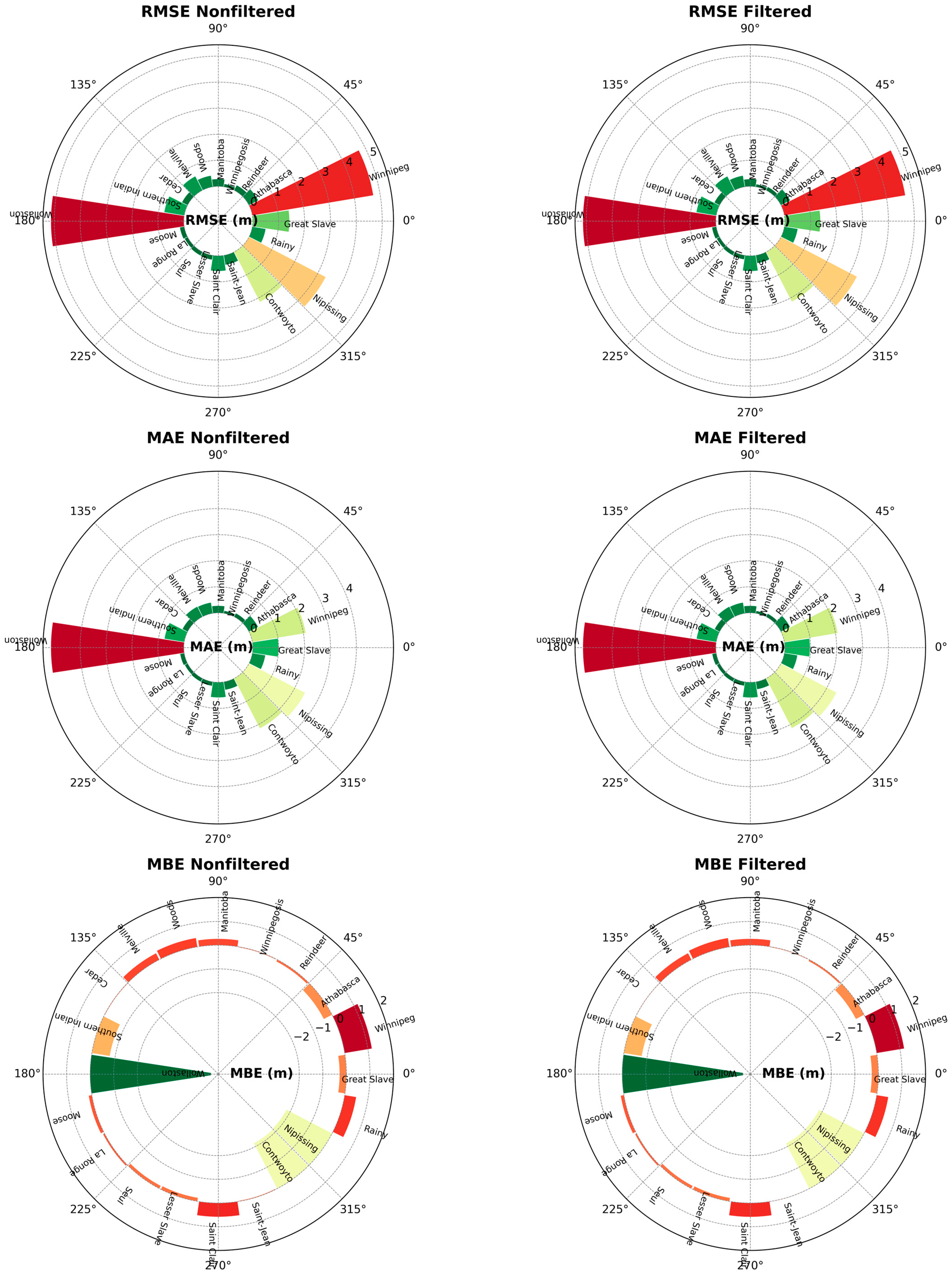
3.1. Error Metric Evaluation and Filtering Effects on ICESat-2 Water Level Estimates

ICESat-2 altimetry-derived water level estimates are evaluated by examining the Root Mean Square Error (RMSE), Mean Absolute Error (MAE), and Mean Bias Error (MBE) for both the filtered and unfiltered datasets. As illustrated in Figure 3, filtering successfully reduces overall error magnitudes, although certain outliers remain, often clustered within a small subset of lakes. For instance, Hylak ID 8130, 2867, and 64 consistently exhibit larger errors in RMSE, MAE, and MBE, suggesting that the measurement inconsistencies may stem from site-specific hydrological or retrieval conditions rather than a broad, systematic bias.

Despite the persistence of these local anomalies, the filtering process substantially improves the overall accuracy of ICESat-2 measurements. When considering all lakes and all observation dates, the mean RMSE decreases from 1.53 m in the unfiltered data to 1.40 m in the filtered data. Excluding the few lakes that exhibit extreme errors reduces the mean RMSE from 1.27 m (unfiltered) to 0.96 m (filtered), demonstrating that a small group of problematic stations disproportionately elevates the overall error metrics. Similar improvements are evident in MAE and MBE, indicating both a reduced overall error and a diminished bias after filtering. The mean MBE of −0.6 m points to a systematic underestimation of water levels compared to the in situ measurements, which may be influenced by factors such as lidar’s penetration at the water surface, suboptimal atmospheric corrections, or potential algorithmic biases.

Figure 4 focuses on the 20 largest lakes and highlights that for most of these water bodies, RMSE and MAE remain below 1.0 m, suggesting that ICESat-2 performs reliably over large, open-water systems. However, Lake Winnipeg and Wollaston Lake show noticeably higher error levels for both RMSE and MAE, implying that local conditions—such as complex shorelines or other hydrodynamic processes—could introduce additional uncertainties. Examining MBE across these large lakes reveals that most do not exhibit a strong bias, yet Lake Winnipeg tends to be positively biased (overestimation), while Wollaston Lake is negatively biased (underestimation). This divergence underscores the potential need for site-specific calibration or additional correction procedures that account for distinctive lake characteristics.

Overall, the results presented in Figure 4 and Figure 5 emphasize that data filtering substantially enhances the accuracy of ICESat-2 water level estimations while exposing certain lakes that demand closer inspection due to their unusually high error values. The fact that most large lakes exhibit relatively low RMSE and MAE demonstrates the broad applicability of ICESat-2 altimetric measurements, yet the outlier lakes highlight how local influences can amplify measurement errors. These findings ultimately suggest that selective filtering coupled with targeted calibration strategies may further refine the accuracy of satellite-derived water levels, particularly in hydrologically or morphologically complex environments.

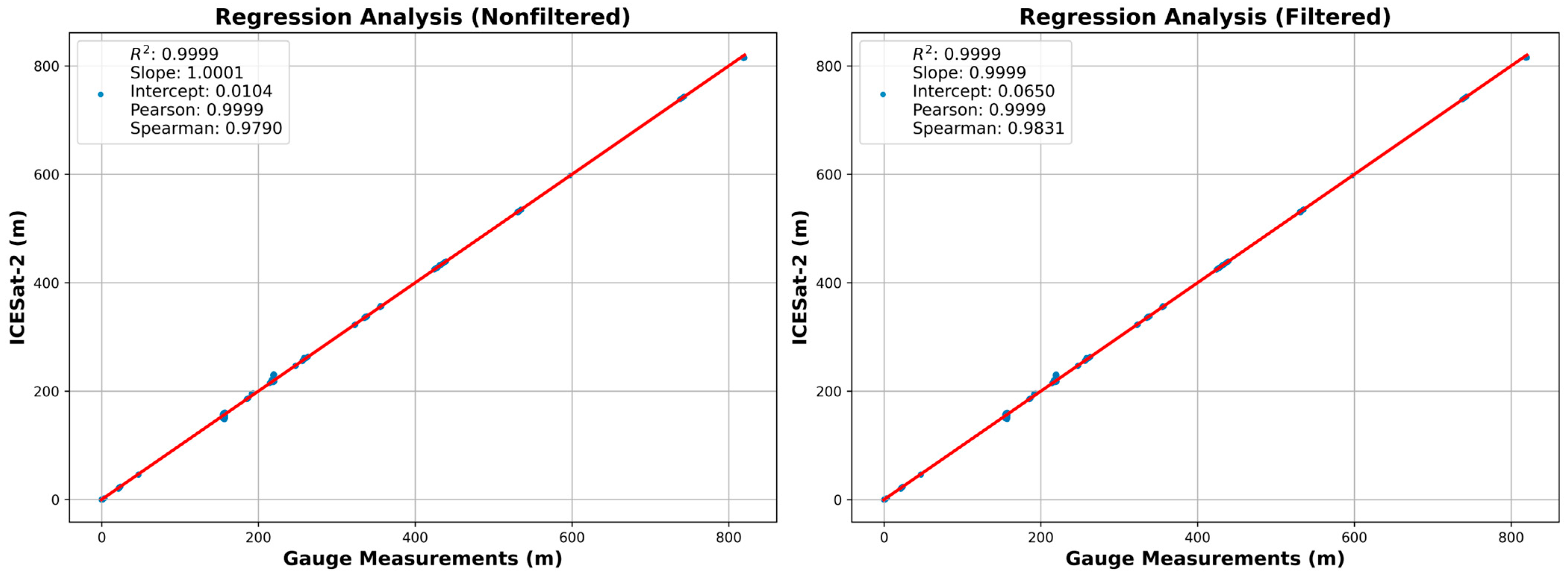
3.2. Regression and Correlation Analysis

ICESat-2-derived water levels were compared against in situ gauge measurements through both regression and correlation analyses applied to unfiltered and filtered datasets. As illustrated in Figure 5, the results demonstrated a near-perfect alignment between satellite estimates and gauge observations, underscoring the high reliability of ICESat-2 altimetry for water level retrieval.

In the linear regression models, the coefficient of determination (R²) reached an exceptionally high value of 0.9999 for both datasets, indicating that nearly all of the variance in the ICESat-2 data was explained by gauge measurements. Moreover, the regression slopes remained close to unity in both the unfiltered and filtered scenarios, suggesting a near 1:1 relationship between the two measurement sources. For the unfiltered dataset, the slope was 1.0001 with an intercept of 0.0104 m, whereas the filtered dataset yielded a slope of 0.9999 and an intercept of 0.0650 m—both indicative of negligible deviations from a perfect fit. These findings confirm the consistency of ICESat-2 measurements with gauge records, while also revealing that filtering introduces only minor adjustments to the absolute water level values.

Correlation metrics further support the robustness of ICESat-2 altimetry. Pearson’s correlation coefficient (r) stood at 0.9999 (p < 0.0001) for both datasets, signifying an almost perfect linear relationship, and Spearman’s rank correlation coefficient (ρ)—which assesses the monotonic order of the observations—improved from 0.9790 to 0.9831 after filtering. This increase indicated that data filtering reduced local anomalies and refined the overall data consistency without compromising the core integrity of the ICESat-2 measurements.

Collectively, these results affirmed that ICESat-2 altimetry provides highly accurate water level estimates in strong agreement with in situ gauges. While the filtering process subtly influences the intercept values, its practical impact on hydrological assessments remains minimal. The enhanced Spearman correlation further demonstrated the merit of targeted filtering in managing localized errors, highlighting the value of such refinements for improving data reliability in diverse aquatic environments.

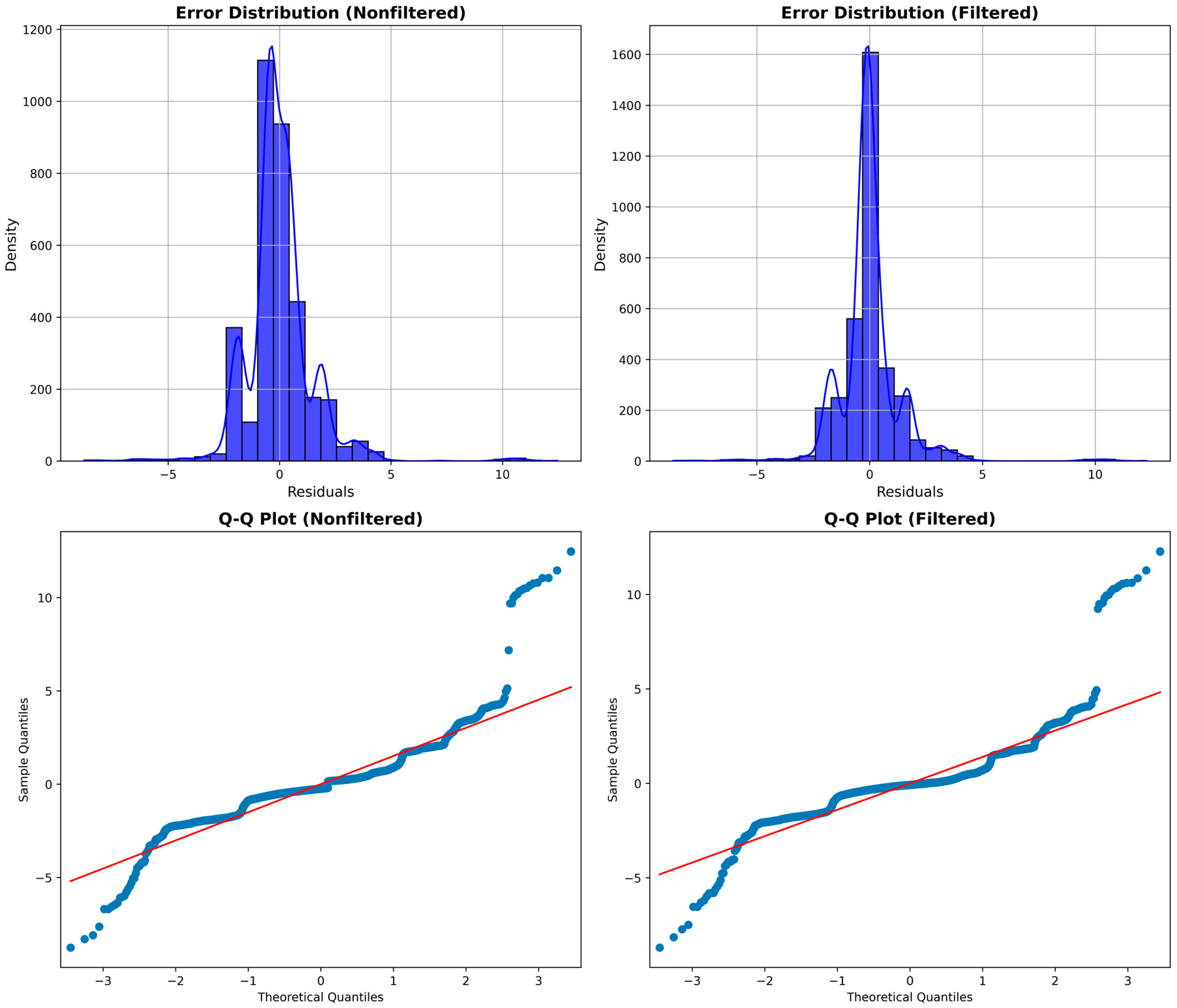
3.3. Error Distribution Characteristics

Residuals from the regression analyses were examined using the Shapiro–Wilk and Kolmogorov–Smirnov tests, alongside histogram, Kernel Density Estimation (KDE), and Q–Q plot evaluations. These procedures were conducted on both unfiltered and filtered datasets, and the combined findings are presented in Figure 6.

The statistical tests (Shapiro–Wilk and Kolmogorov–Smirnov) return p-values of 0.0000 for both the unfiltered and filtered datasets, suggesting that the residuals in neither dataset strictly follow a normal distribution. In the histogram and KDE plots, unfiltered residuals appear more dispersed, featuring heavier tails and a greater presence of outliers. By contrast, filtering reduces these extreme values, resulting in a narrower, more concentrated distribution, though some skewness remains. Q–Q plots reinforce these observations. While the bulk of the points in the filtered dataset align reasonably well with the theoretical normal line, a number of data points still deviate in the tails, reflecting persistent departures from ideal normality. Notably, these outliers often correspond to the same lakes identified in earlier sections, where highly irregular shorelines and potentially unrepresentative gauge stations may introduce additional variability. Although these deviations indicate that standard assumptions of linear regression may not be perfectly met, the overall performance of the ICESat-2 water level estimation remains robust, particularly for the majority of lakes where the residuals are relatively well behaved. In instances where coastline complexity or other site-specific factors play a larger role, further refinements such as data transformations, robust regression methods, or site-specific calibrations could help to refine residual distributions without detracting from the broader reliability of the approach.

In summary, while the residuals are not strictly normal in either dataset, the filtering process markedly reduces outliers, bringing most data points closer to a normal-like distribution. The persistent deviations observed largely arise from a small subset of lakes with intricate shoreline morphologies. Recognizing and accounting for these localized conditions can enhance model performance and ensure that the strong agreement between ICESat-2 and gauge-derived water levels extends across a range of hydrological settings.

3.4. Spatial Variability of Errors

In order to explore how various hydrological characteristics may influence the accuracy of ICESat-2-derived water levels, RMSE was examined in relation to lake area, depth, and elevation. Figure 7 presents these three relationships with red regression lines highlighting the overall trends. The log-scaled plot of lake area reveals that larger lakes tend to exhibit lower and more stable RMSE values, while smaller lakes display substantial variation, including a few extreme error cases. Although there is a slight upward trend in the regression curve, considerable uncertainty remains for very large lakes, suggesting that other local factors may also affect these errors. One plausible explanation is that ICESat-2′s measurement footprint may capture limited coverage in smaller lakes, making edge effects more pronounced and thus increasing errors. In contrast, larger lakes benefit from a broader range of satellite observations, effectively smoothing out local anomalies and reducing overall RMSE.

Further analysis of RMSE values in the context of average lake depth indicates that shallow lakes (particularly those with depths of 0–30 m) are prone to greater measurement variability. Elevated surface disturbance, turbidity, and other near-surface processes in these shallow environments could explain the higher error magnitudes. Although deeper lakes typically yield more consistent, lower RMSE values, outliers persist in certain cases, implying that localized conditions—such as complex bathymetry or specific environmental factors—may affect measurement precision. The regression line suggests a modest upward trend in RMSE as depth increases, but the widespread distribution of data points complicates conclusive interpretations.

When examining elevation, the data indicate that lower lying lakes generally show wider variations in RMSE, whereas higher elevation lakes tend to have fewer errors. The negative slope in the regression line aligns with a potential reduction in environmental and atmospheric interference at higher altitudes, where conditions may be more stable and involve less anthropogenic or vegetation-related noise. At lower elevations, factors such as urban development, agricultural practices, or heavier vegetation cover could introduce additional challenges, thereby increasing measurement uncertainty.

Collectively, these observations point to a non-uniform distribution of ICESat-2 errors, governed by geographical and hydrological properties. Larger, deeper, and higher elevation lakes generally exhibit more favorable outcomes, while smaller, shallower, and low-elevation lakes may pose greater challenges for satellite measurements. These findings highlight the potential value of developing adaptive approaches that account for the unique features of individual lakes, ultimately enhancing the reliability of ICESat-2-derived water level estimates.

3.5. Effect of Lidar Point Density on Accuracy

The scatterplot in Figure 8 illustrates how changes in photon density (points/m²) can influence RMSE values in ICESat-2-derived water levels. Although a higher density of laser returns is often assumed to enhance precision, the observed relationship here is more nuanced. At relatively low photon densities (roughly 1–10 points/m²), RMSE remains stable—typically ranging from 0 to 2 m—and exhibits a narrow confidence interval, suggesting minimal uncertainty in this regime. Increasing photon density within this lower range does not consistently reduce RMSE further, implying that beyond a certain threshold, additional photon returns may not substantially improve measurement accuracy.

A moderate rise in photon density (around 10–30 points/m²) generally coincides with low RMSE values, often below 1 m. However, the spread of data points broadens, and several cases display unexpectedly high errors. Environmental factors—such as localized water surface conditions, the presence of unaccounted reflectors, and variations in atmospheric interference—can drive this variability. Although it might be expected that more photons would always yield more reliable retrievals, these findings highlight the interplay of multiple influences. Higher photon density does appear beneficial in many instances, yet other site-specific conditions can overshadow the advantage it provides, thereby increasing overall uncertainty.

A more counterintuitive trend emerges at very high photon densities (exceeding about 30 points/m²), where RMSE rises sharply in some lakes. The regression curve bends upward, and the confidence interval widens substantially, underscoring a growing unpredictability in the measurement process. This pattern may reflect signal saturation, wherein an overabundance of photon returns leads to data-processing challenges or an enhanced susceptibility to noise. The combined effect could ultimately inflate RMSE estimates rather than reduce them. Taken together, these observations indicate that while photon density does contribute to measurement quality, it is far from the sole determinant. Surface roughness, water clarity, regional atmospheric conditions, and the calibration of retrieval algorithms also play important roles in shaping the accuracy of satellite altimetry. As a result, there may be an optimal photon density range that balances the benefits of additional data points against the risks of processing complexity and noise.

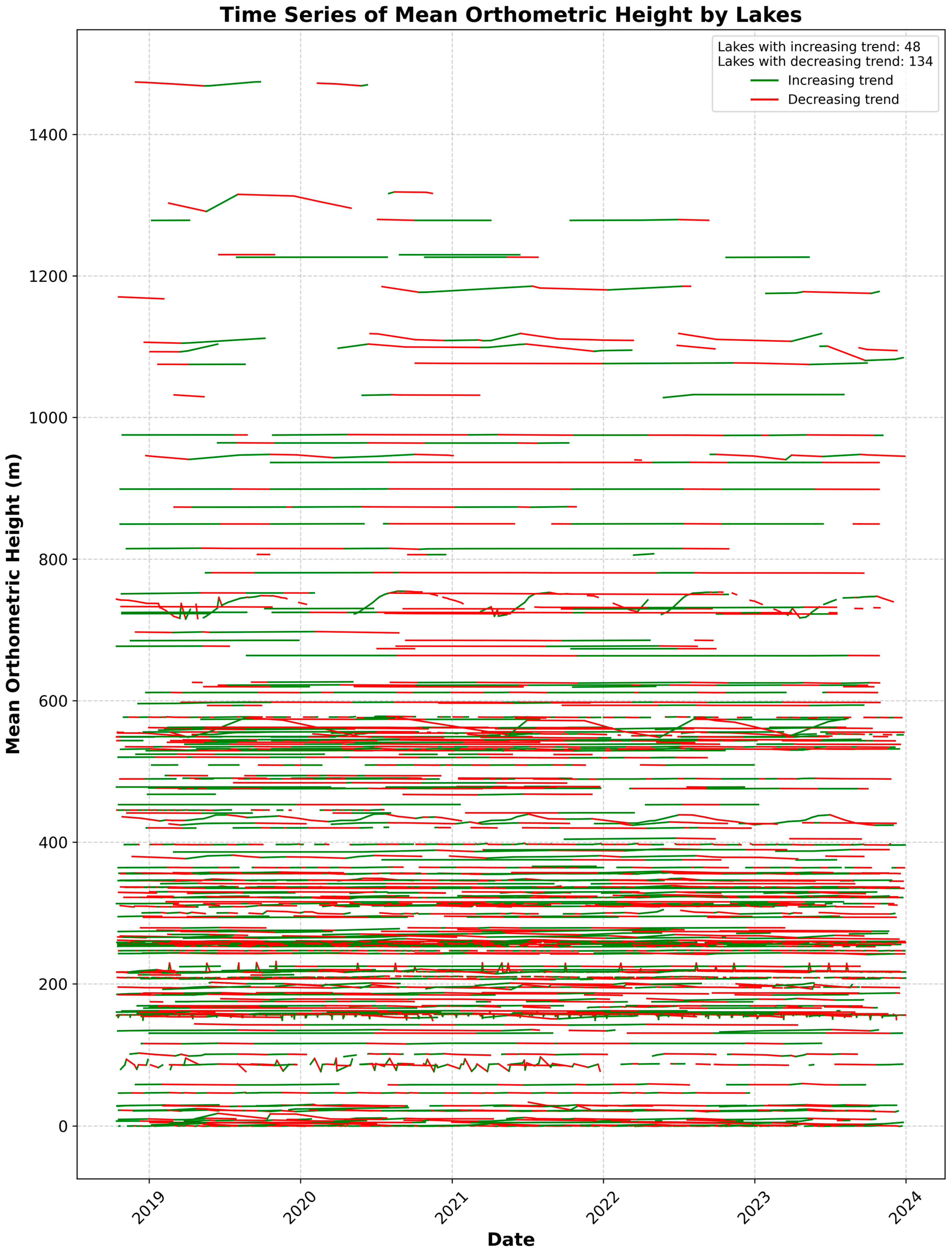
3.6. Temporal Variability of Water Levels

The temporal evolution of lake water levels provides essential insights into hydrological dynamics, potential climate influences, and anthropogenic pressures. As illustrated in Figure 9, which plots the time series of Mean Orthometric Height for a large set of lakes, the data reveal a pronounced prevalence of declining trends (red lines) over increasing ones (green lines). Specifically, 134 lakes exhibit a downward trajectory, while only 48 show sustained increases. This imbalance highlights a broader pattern of water level reductions, suggesting that many lakes are under stress from factors such as reduced inflows, enhanced evaporation, or intensified water extraction.

A striking observation is the wide range of mean orthometric heights, spanning from below 200 m to above 1400 m. Although high-elevation lakes (those exceeding approximately 1000 m) tend to remain relatively stable, low-elevation lakes appear more prone to fluctuations and pronounced declines. These differences may be attributable to greater anthropogenic impacts in lower lying regions, such as agricultural water withdrawals or urban development, as well as potential climatic factors that differentially affect environments at various altitudes [58]. In contrast, lakes situated at higher elevations may benefit from less intensive land use or more predictable meltwater inputs, resulting in fewer abrupt changes [59].

Seasonal and interannual variability also emerges from the time series, with some lakes exhibiting short-lived increases followed by longer term declines. These dynamics could stem from episodic rainfall events, rapidly changing atmospheric conditions, or localized management strategies such as controlled reservoir releases [60]. Even within the same elevation bands, adjacent lakes can exhibit diverging patterns, suggesting that geographically specific drivers, whether climatic, hydrological, or human-induced, play a significant role in shaping water level trajectories [61].

Overall, the dominance of downward trends raises concerns about long-term water resource sustainability and ecosystem resilience, particularly in regions where a steady decrease in lake levels may indicate prolonged drought, diminished groundwater contributions, or shifts in precipitation regimes. Continued monitoring and refined analyses that integrate climate data, land use patterns, and hydrological modeling would help to clarify the underlying processes governing these trends [62,63]. Figure 9 offers a vital window into these changes, underscoring the need to address both natural variability and human impacts when managing and conserving lake systems over time.

4. Conclusions

This study presents a comprehensive assessment of ICESat-2 ATL13 altimetry for estimating water levels in Canadian lakes that exhibit a wide range of morphological characteristics. By integrating satellite observations, in situ gauge data, and HydroLAKES-based spatial filtering, our analysis demonstrates that ICESat-2 is a valuable tool for inland water monitoring. The notable reduction in RMSE from 1.53 m in the unfiltered dataset to 1.40 m following the application of HydroLAKES filtering, and a further reduction to 0.96 m when outlier lakes were excluded, strongly underscores the importance and effectiveness of high-resolution spatial refinement in enhancing measurement accuracy.

A detailed evaluation of the data reveals that while a majority of lakes, particularly those that are larger and deeper, yield stable and reliable altimetric estimates, smaller lakes with complex shorelines remain challenging. The increased variability observed in these smaller systems suggests that the intricate interactions between lake morphology and photon return characteristics can introduce biases that are not fully mitigated by standard filtering techniques. This finding emphasizes the need for site-specific calibration protocols that account for unique geomorphological features. Furthermore, although the overall statistical agreement between ICESat-2 measurements and in situ observations is remarkably high (R² = 0.9999), the unexpected increase in RMSE at high photon densities indicates that current retrieval algorithms may require further refinement. This issue is particularly critical in dense photon return environments, where the signal complexity can degrade the precision of water level estimates.

Temporal trend analysis further reveals a pronounced asymmetry in water level changes, with 134 lakes exhibiting declining levels compared to only 48 lakes showing increases. This disparity raises important questions regarding the underlying drivers of these trends, which may include a combination of climate variability, regional hydrological alterations, and anthropogenic impacts. The observed declines in water levels could be indicative of broader environmental shifts that warrant more detailed investigation, especially in the context of climate adaptation and freshwater ecosystem management.

The implications of our findings extend beyond the immediate results of error reduction and trend detection. They suggest that the integration of satellite-based altimetry with advanced spatial filtering techniques, such as those provided by the HydroLAKES database, holds significant promise for enhancing the monitoring of inland water bodies on a regional to global scale. However, several limitations and challenges persist. For example, the reliance on in situ gauge data for calibration purposes, while beneficial for validation, is constrained by the spatial distribution of these gauges, which are often sparse in remote regions. Moreover, the dynamic nature of lake morphologies over time—driven by seasonal, interannual, and long-term climatic factors—necessitates the development of adaptive filtering methods that can evolve in tandem with these changes.

Looking forward, future investigations should prioritize several key areas of research. First, multi-sensor integration remains a promising avenue; combining ICESat-2 altimetry with complementary observations from other LiDAR altimeters such as GEDI and high-resolution optical imagery could further enhance both the spatial and temporal resolution of water level monitoring. Second, the development of machine-learning-based error correction models is essential. Such models could dynamically adjust for variations in lake morphology and environmental conditions, thereby improving the robustness of altimetric measurements. Third, expanding the network of in situ validation sites, particularly in regions where data are currently limited, would strengthen calibration frameworks and enhance the overall reliability of satellite-derived estimates. Additionally, extending the temporal range of observations to capture decadal-scale hydrological changes would provide deeper insights into the long-term impacts of climate variability and anthropogenic activities on freshwater resources.

Finally, refining of the spatial filtering approaches based on the HydroLAKES database warrants further research. Advanced filtering techniques that can better address irregular lake boundaries and mixed land–water pixels are needed to minimize the errors associated with complex shoreline geometries. By systematically addressing these challenges, future studies can build upon the present work to develop more sophisticated remote monitoring methodologies that not only improve measurement accuracy but also offer richer insights into the hydrological dynamics of inland water bodies.

In summary, by leveraging ICESat-2 altimetry alongside HydroLAKES spatial filtering and complementary data-processing strategies, this study reinforces the pivotal role of satellite-based observations in contemporary hydrological science. Our results offer critical insights for water resource management, inform climate adaptation strategies, and contribute to the broader understanding of freshwater ecosystem conservation in the face of environmental change.

References

1. Whitehead, P.G.; Wilby, R.L.; Battarbee, R.W.; Kernan, M.; Wade, A.J. A review of the potential impacts of climate change on surface water quality. Hydrol. Sci. J. 2009, 54, 101–123. [Google Scholar] [CrossRef]
2. Hao, H.; Yao, J.; Chen, Y.; Xu, J.; Li, Z.; Duan, W.; Ismail, S.; Wang, G. Ecological transitions in Xinjiang, China: Unraveling the impact of climate change on vegetation dynamics (1990–2020). J. Geogr. Sci. 2024, 34, 1039–1064. [Google Scholar] [CrossRef]
3. Williamson, C.E.; Saros, J.E.; Vincent, W.F.; Smol, J.P. Lakes and reservoirs as sentinels, integrators, and regulators of climate change. Limnol. Oceanogr. 2009, 54, 2273–2282. [Google Scholar] [CrossRef]
4. Heino, J.; Alahuhta, J.; Bini, L.M.; Cai, Y.; Heiskanen, A.S.; Hellsten, S.; Angeler, D.G. Lakes in the era of global change: Moving beyond single-lake thinking in maintaining biodiversity and ecosystem services. Biol. Rev. 2021, 96, 89–106. [Google Scholar] [CrossRef]
5. Xiao, Q.; Xu, X.; Qi, T.; Luo, J.; Lee, X.; Duan, H. Lakes shifted from a carbon dioxide source to a sink over past two decades in China. Sci. Bull. 2024, 69, 1857–1861. [Google Scholar] [CrossRef]
6. Wu, C.; Wu, X.; Lu, C.; Sun, Q.; He, X.; Yan, L.; Qin, T. Characteristics and driving factors of lake level variations by climatic factors and groundwater level. J. Hydrol. 2022, 608, 127654. [Google Scholar] [CrossRef]
7. Raihan, A. A review of the global climate change impacts, adaptation strategies, and mitigation options in the socio-economic and environmental sectors. J. Environ. Sci. Econ. 2023, 2, 36–58. [Google Scholar]
8. Adebisi, N.; Balogun, A.L.; Min, T.H.; Tella, A. Advances in estimating sea level rise: A review of tide gauge, satellite altimetry and spatial data science approaches. Ocean Coast. Manag. 2021, 208, 105632. [Google Scholar] [CrossRef]
9. Ren, H.; Cromwell, E.; Kravitz, B.; Chen, X. Using long short-term memory models to fill data gaps in hydrological monitoring networks. Hydrol. Earth Syst. Sci. 2022, 26, 1727–1743. [Google Scholar] [CrossRef]
10. Fassoni-Andrade, A.C.; Fleischmann, A.S.; Papa, F.; Paiva, R.C.D.D.; Wongchuig, S.; Melack, J.M.; Pellet, V. Amazon hydrology from space: Scientific advances and future challenges. Rev. Geophys. 2021, 59, e2020RG000728. [Google Scholar] [CrossRef]
11. Huang, Z.; Sun, R.; Wang, H.; Wu, X. Trends and innovations in surface water monitoring via satellite altimetry: A 34-year bibliometric review. Remote Sens. 2024, 16, 2886. [Google Scholar] [CrossRef]
12. Frappart, F.; Blarel, F.; Fayad, I.; Bergé-Nguyen, M.; Crétaux, J.F.; Shu, S.; Baghdadi, N. Evaluation of the performances of radar and lidar altimetry missions for water level retrievals in mountainous environment: The case of the Swiss lakes. Remote Sens. 2021, 13, 2196. [Google Scholar] [CrossRef]
13. Kossieris, S.; Tsiakos, V.; Tsimiklis, G.; Amditis, A. Inland water level monitoring from satellite observations: A scoping review of current advances and future opportunities. Remote Sens. 2024, 16, 1181. [Google Scholar] [CrossRef]
14. Ross, N.; Rostami, A.; Lee, H.; Chang, C.H.; Hossain, F.; Milillo, P.; Towashiraporn, P. Monitoring reservoir water elevation changes using Jason-2/3 altimetry satellite missions: Exploring the capabilities of JASTER (Jason-2/3 Altimetry Stand-Alone Tool for Enhanced Research). Int. J. Digit. Earth 2024, 17, 2406387. [Google Scholar]
15. Moreau, T.; Cadier, E.; Boy, F.; Aublanc, J.; Rieu, P.; Raynal, M.; Mavrocordatos, C. High-performance altimeter Doppler processing for measuring sea level height under varying sea state conditions. Adv. Space Res. 2021, 67, 1870–1886. [Google Scholar]
16. Kwok, R.; Cunningham, G.F.; Zwally, H.J.; Yi, D. Ice, Cloud, and land Elevation Satellite (ICESat) over Arctic sea ice: Retrieval of freeboard. J. Geophys. Res. Ocean. 2007, 112, C12013. [Google Scholar] [CrossRef]
17. Schutz, B.E.; Zwally, H.J.; Shuman, C.A.; Hancock, D.; DiMarzio, J.P. Overview of the ICESat mission. Geophys. Res. Lett. 2005, 32, 21. [Google Scholar]
18. Urban, T.J.; Schutz, B.E.; Neuenschwander, A.L. A survey of ICESat coastal altimetry applications: Continental coast, open ocean island, and inland river. Terr. Atmos. Ocean. Sci. 2008, 19, 1–19. [Google Scholar]
19. Shu, L.; Jiang, Q.; Zhang, X.; Zhao, K. Potential and limitations of satellite laser altimetry for monitoring water surface dynamics: ICESat for US lakes. Int. J. Agric. Biol. Eng. 2017, 10, 154–165. [Google Scholar] [CrossRef]
20. Martino, A.J.; Neumann, T.A.; Kurtz, N.T.; McLennan, D. ICESat-2 mission overview and early performance. In Proceedings of the Sensors, Systems, and Next-Generation Satellites XXIII, Strasbourg, France, 9–12 September 2019; Volume 11151, pp. 68–77. [Google Scholar]
21. Smith, B.; Fricker, H.A.; Holschuh, N.; Gardner, A.S.; Adusumilli, S.; Brunt, K.M.; Siegfried, M.R. Land ice height-retrieval algorithm for NASA’s ICESat-2 photon-counting laser altimeter. Remote Sens. Environ. 2019, 233, 111352. [Google Scholar]
22. Ryan, J.C.; Smith, L.C.; Cooley, S.W.; Pitcher, L.H.; Pavelsky, T.M. Global characterization of inland water reservoirs using ICESat-2 altimetry and climate reanalysis. Geophys. Res. Lett. 2020, 47, e2020GL088543. [Google Scholar] [CrossRef]
23. Yuan, C.; Gong, P.; Bai, Y. Performance assessment of ICESat-2 laser altimeter data for water-level measurement over lakes and reservoirs in China. Remote Sens. 2020, 12, 770. [Google Scholar] [CrossRef]
24. Narin, O.G.; Abdikan, S. Multi-temporal analysis of inland water level change using ICESat-2 ATL-13 data in lakes and dams. Environ. Sci. Pollut. Res. 2023, 30, 15364–15376. [Google Scholar]
25. Chen, T.; Song, C.; Luo, S.; Ke, L.; Liu, K.; Zhu, J. Monitoring global reservoirs using ICESat-2: Assessment on spatial coverage and application potential. J. Hydrol. 2022, 604, 127257. [Google Scholar]
26. Markus, T.; Neumann, T.; Martino, A.; Abdalati, W.; Brunt, K.; Csatho, B.; Zwally, J. The Ice, Cloud, and Land Elevation Satellite-2 (ICESat-2): Science requirements, concept, and implementation. Remote Sens. Environ. 2017, 190, 260–273. [Google Scholar]
27. Dietrich, J.T.; Magruder, L.A.; Holwill, M. Monitoring coastal waves with ICESat-2. J. Mar. Sci. Eng. 2023, 11, 2082. [Google Scholar] [CrossRef]
28. Kui, M.; Xu, Y.; Wang, J.; Cheng, F. Research on the adaptability of typical denoising algorithms based on ICESat-2 data. Remote Sens. 2023, 15, 3884. [Google Scholar] [CrossRef]
29. Xie, J.; Li, B.; Jiao, H.; Zhou, Q.; Mei, Y.; Xie, D.; Fu, Y. Water level change monitoring based on a new denoising algorithm using data from Landsat and ICESat-2: A case study of Miyun Reservoir in Beijing. Remote Sens. 2022, 14, 4344. [Google Scholar] [CrossRef]
30. Han, K.; Kim, S.; Mehrotra, R.; Sharma, A. Enhanced water level monitoring for small and complex inland water bodies using multi-satellite remote sensing. Environ. Model. Softw. 2024, 180, 106169. [Google Scholar]
31. Messager, M.L.; Lehner, B.; Grill, G.; Nedeva, I.; Schmitt, O. Estimating the volume and age of water stored in global lakes using a geo-statistical approach. Nat. Commun. 2016, 7, 13603. [Google Scholar]
32. Han, W.; Huang, C.; Gu, J.; Hou, J.; Zhang, Y.; Wang, W. Water level change of Qinghai Lake from ICESat and ICESat-2 laser altimetry. Remote Sens. 2022, 14, 6212. [Google Scholar] [CrossRef]
33. Liu, C.; Hu, R.; Wang, Y.; Lin, H.; Zeng, H.; Wu, D.; Shao, C. Monitoring water level and volume changes of lakes and reservoirs in the Yellow River Basin using ICESat-2 laser altimetry and Google Earth Engine. J. Hydro-Environ. Res. 2022, 44, 53–64. [Google Scholar]
34. Braun, A.; Cheng, K.C.; Csatho, B.; Shum, C.K. ICESat laser altimetry in the Great Lakes. In Proceedings of the 60th Annual Meeting of the Institute of Navigation, Dayton, OH, USA, 7–9 June 2004; pp. 409–416. [Google Scholar]
35. Xiang, J.; Li, H.; Zhao, J.; Cai, X.; Li, P. Inland water level measurement from spaceborne laser altimetry: Validation and comparison of three missions over the Great Lakes and lower Mississippi River. J. Hydrol. 2021, 597, 126312. [Google Scholar]
36. Balsamo, G.; Agusti-Panareda, A.; Albergel, C.; Arduini, G.; Beljaars, A.; Bidlot, J.; Blyth, E.; Bousserez, N.; Boussetta, S.; Brown, A.; et al. Satellite and In Situ Observations for Advancing Global Earth Surface Modelling: A Review. Remote Sens. 2018, 10, 2038. [Google Scholar] [CrossRef]
37. Du, J.; Watts, J.D.; Jiang, L.; Lu, H.; Cheng, X.; Duguay, C.; Farina, M.; Qiu, Y.; Kim, Y.; Kimball, J.S.; et al. Remote sensing of environmental changes in cold regions: Methods, achievements and challenges. Remote Sens. 2019, 11, 1952. [Google Scholar] [CrossRef]
38. Erler, A.R. High Resolution Hydro-Climatological Projections for Western Canada; University of Toronto: Toronto, ON, Canada, 2015. [Google Scholar]
39. Curran, J.H.; Biles, F.E. Identification of seasonal streamflow regimes and streamflow drivers for daily and peak flows in Alaska. Water Resour. Res. 2021, 57, e2020WR028425. [Google Scholar]
40. Rawson, D.S. The bottom fauna of Great Slave Lake. J. Fish. Board Can. 1953, 10, 486–520. [Google Scholar]
41. Stewardship, M.W. State of Lake Winnipeg: 1999 to 2007; Environment Canada and Manitoba Water Stewardship: Winnipeg, MB, Canada, 2011. [Google Scholar]
42. Desloges, J.R.; Gilbert, R. Sedimentary record of Harrison Lake: Implications for deglaciation in southwestern British Columbia. Can. J. Earth Sci. 1991, 28, 800–815. [Google Scholar]
43. Landals, A.J. The Lake Minnewanka Site: Patterns in Late Pleistocene Use of the Albarta Rocky Mountains; University of Calgary: Calgary, AB, USA, 2008. [Google Scholar]
44. Quartly, G.D.; Rinne, E.; Passaro, M.; Andersen, O.B.; Dinardo, S.; Fleury, S.; Guillot, A.; Hendricks, S.; Kurekin, A.A.; Müller, F.L.; et al. Retrieving sea level and freeboard in the Arctic: A review of current radar altimetry methodologies and future perspectives. Remote Sens. 2019, 11, 881. [Google Scholar] [CrossRef]
45. Neumann, T.A.; Brenner, A.; Hancock, D.; Robbins, J.; Saba, J.; Harbeck, K.; Gibbons, A.; Lee, J.; Luthcke, S.B.; Rebold, T.; et al. ATLAS/ICESat-2 L2A Global Geolocated Photon Data, Version 3; NASA National Snow and Ice Data Center Distributed Active Archive Center: Boulder, CO, USA, 2021. [Google Scholar]
46. Lehner, B.; Grill, G. Global river hydrography and network routing: Baseline data and new approaches to study the world’s large river systems. Hydrol. Process. 2013, 27, 2171–2186. [Google Scholar]
47. Pietroniro, A.; Peters, D.L.; Yang, D.; Fiset, J.M.; Saint-Jean, R.; Fortin, V.; Leconte, R.; Bergeron, J.; Siles, G.L.; Trudel, M.; et al. Canada’s Contributions to the SWOT Mission-Terrestrial Hydrology (SWOT-C TH). Can. J. Remote Sens. 2019, 45, 116–138. [Google Scholar] [CrossRef]
48. National Water Data Archive, Water Level and Flow. Water Office of Canada. Available online: https://wateroffice.ec.gc.ca (accessed on 7 February 2025).
49. Singh, V.P.; Singh, R.; Paul, P.K.; Bisht, D.S.; Gaur, S. Hydrological Processes Modelling and Data Analysis; Water Science and Technology Library; Springer: Singapore, 2024; Volume 127. [Google Scholar]
50. Wan, X.; Wang, W.; Liu, J.; Tong, T. Estimating the sample mean and standard deviation from the sample size, median, range and/or interquartile range. BMC Med. Res. Methodol. 2014, 14, 135. [Google Scholar] [CrossRef] [PubMed]
51. Chapaneri, R.; Shah, S. Multi-level Gaussian mixture modeling for detection of malicious network traffic. J. Supercomput. 2021, 77, 4618–4638. [Google Scholar] [CrossRef]
52. Shen, W.; Chen, S.; Xu, J.; Zhang, Y.; Liang, X.; Zhang, Y. Enhancing Extreme Precipitation Forecasts through Machine Learning Quality Control of Precipitable Water Data from Satellite FengYun-2E: A Comparative Study of Minimum Covariance Determinant and Isolation Forest Methods. Remote Sens. 2024, 16, 3104. [Google Scholar] [CrossRef]
53. Helsel, D.R. Less than obvious-statistical treatment of data below the detection limit. Environ. Sci. Technol. 1990, 24, 1766–1774. [Google Scholar] [CrossRef]
54. Chai, T.; Draxler, R.R. Root mean square error (RMSE) or mean absolute error (MAE). Geosci. Model Dev. Discuss. 2014, 7, 1525–1534. [Google Scholar]
55. Hu, X.; Xie, Z.; Liu, F. Assessment of speckle pattern quality in digital image correlation from the perspective of mean bias error. Measurement 2021, 173, 108618. [Google Scholar] [CrossRef]
56. Aalen, O.O. A linear regression model for the analysis of life times. Stat. Med. 1989, 8, 907–925. [Google Scholar] [CrossRef]
57. De Winter, J.C.; Gosling, S.D.; Potter, J. Comparing the Pearson and Spearman correlation coefficients across distributions and sample sizes: A tutorial using simulations and empirical data. Psychol. Methods 2016, 21, 273. [Google Scholar] [CrossRef]
58. Zonn, I.S.; Glantz, M.; Kosarev, A.N.; Kostianoy, A.G. The Aral Sea Encyclopedia; Springer Science & Business Media: Berlin/Heidelberg, Germany, 2009. [Google Scholar]
59. Woolway, R.I.; Kraemer, B.M.; Lenters, J.D.; Merchant, C.J.; O’Reilly, C.M.; Sharma, S. Global lake responses to climate change. Nat. Rev. Earth Environ. 2020, 1, 388–403. [Google Scholar] [CrossRef]
60. Geris, J.; Comte, J.C.; Franchi, F.; Petros, A.K.; Tirivarombo, S.; Selepeng, A.T.; Villholth, K.G. Surface water-groundwater interactions and local land use control water quality impacts of extreme rainfall and flooding in a vulnerable semi-arid region of Sub-Saharan Africa. J. Hydrol. 2022, 609, 127834. [Google Scholar]
61. Ji, P.; Su, R.; Wu, G.; Xue, L.; Zhang, Z.; Fang, H.; Gao, R.; Zhang, W.; Zhang, D. Projecting Future Wetland Dynamics Under Climate Change and Land Use Pressure: A Machine Learning Approach Using Remote Sensing and Markov Chain Modeling. Remote Sens. 2025, 17, 1089. [Google Scholar] [CrossRef]
62. Pielke Sr, R.A.; Pitman, A.; Niyogi, D.; Mahmood, R.; McAlpine, C.; Hossain, F.; Goldewijk, K.K.; Nair, U.; Betts, R.; Fall, S.; et al. Land use/land cover changes and climate: Modeling analysis and observational evidence. Wiley Interdiscip. Rev. Clim. Change 2011, 2, 828–850. [Google Scholar] [CrossRef]
63. Fatichi, S.; Vivoni, E.R.; Ogden, F.L.; Ivanov, V.Y.; Mirus, B.; Gochis, D.; Downer, C.W.; Camporese, M.; Davison, J.H.; Ebel, B.; et al. An overview of current applications, challenges, and future trends in distributed process-based models in hydrology. J. Hydrol. 2016, 537, 45–60. [Google Scholar]
Figure 1. Geographic distribution of the lakes used in this study.
Water 17 01098 g001
Figure 2. Relationship between the lake elevation and average depth for the 182 lakes analyzed in this study.
Water 17 01098 g002
Figure 3. Distribution of RMSE, MAE, and MBE values for both filtered and unfiltered ICESat-2-derived water levels compared to in situ gauge measurements.
Water 17 01098 g003
Figure 4. Polar plots of RMSE, MAE, and MBE for the 20 largest lakes, comparing nonfiltered (left) and filtered (right) datasets.
Water 17 01098 g004
Figure 5. Linear regression comparisons between ICESat-2-derived water levels and gauge measurements for unfiltered (left) and filtered (right) datasets.
Water 17 01098 g005
Figure 6. Residual distribution analysis—histogram, KDE, and Q-Q Plots for unfiltered and filtered data.
Water 17 01098 g006
Figure 7. Influence of lake characteristics on RMSE.
Water 17 01098 g007
Figure 8. Influence of photon density on RMSE.
Water 17 01098 g008
Figure 9. Temporal trends in mean orthometric height of lakes (2018–2024).
Water 17 01098 g009