Abstract
This study proposes an innovative framework integrating geographic information systems (GISs), water quality index (WQI) analysis, and advanced machine learning (ML) models to evaluate the prevalence and impact of organic and inorganic pollutants across the urban–industrial confluence zones (UICZ) surrounding the National Capital Territory (NCT) of India. Surface water samples (n = 118) were systematically collected from the Gautam Buddha Nagar, Ghaziabad, Faridabad, Sonipat, Gurugram, Jhajjar, and Baghpat districts to assess physical, chemical, and microbiological parameters. The application of spatial interpolation techniques, such as kriging and inverse distance weighting (IDW), enhances WQI estimation in unmonitored areas, improving regional water quality assessments and remediation planning. GIS mapping highlighted stark spatial disparities, with industrial hubs, like Faridabad and Gurugram, exhibiting WQI values exceeding 600 due to untreated industrial discharges and wastewater, while rural regions, such as Jhajjar and Baghpat, recorded values below 200, reflecting minimal anthropogenic pressures. The study employed four ML models—linear regression (LR), random forest (RF), Gaussian process regression (GPR), and support vector machines (SVM)—to predict WQI with high precision. SVM_Poly emerged as the most effective model, achieving testing CC, RMSE, and MAE values of 0.9997, 11.4158, and 5.6085, respectively, outperforming RF (0.9925, 29.8107, 21.7398) and GPR_PUK (0.9811, 68.4466, 54.0376). By leveraging machine learning models, this study enhances WQI prediction beyond conventional computation, enabling spatial extrapolation and early contamination detection in data-scarce regions. Sensitivity analysis identified total suspended solids as the most critical predictor influencing WQI, underscoring its relevance in monitoring programs. This research uniquely integrates ML algorithms with spatial analytics, providing a novel methodological contribution to water quality assessment. The findings emphasize the urgency of mitigating the fate and transport of organic and inorganic pollutants to protect Delhi’s hydrological ecosystems, presenting a robust decision-support system for policymakers and environmental managers.
1. Introduction
Water quality is fundamental to environmental sustainability and human well-being. Freshwater resources sustain biodiversity, regulate ecosystems, and provide crucial services for agriculture, industry, and domestic needs. However, pollution-induced deterioration of water quality significantly impacts public health, leading to waterborne morbidity and mortality along with a huge number of out-of-pocket expenditures. On a global scale, contaminated water accounts for approximately 485,000 deaths annually due to diarrheal diseases [1]. Furthermore, polluted water systems disrupt aquatic ecosystems, causing habitat degradation and biodiversity loss [2]. Economic activities are also adversely affected, with industries reliant on clean water encountering increased treatment expenses and operational difficulties. Agricultural productivity suffers as well, as elevated salinity and chemical pollutants degrade soil health and reduce crop yields [3]. Addressing these concerns is vital to achieving sustainable development. The combined effects of rapid industrialization, urbanization, and agricultural growth have placed immense strain on global water resources. Nearly 80% of wastewater is released untreated into natural water bodies, resulting in the contamination of rivers, lakes, and groundwater [4]. Urban centers contribute a mix of organic and chemical pollutants from untreated sewage, while agricultural practices introduce pesticides, fertilizers, and sediments [5]. These pollutants lead to eutrophication, reduced dissolved oxygen levels, and increased turbidity, ultimately compromising the usability of water resources. Integrated water quality assessment, encompassing physical, chemical, and microbiological analyses, is crucial for identifying contamination hotspots and enabling effective policy measures [6].
Delhi and its surrounding districts, including Sonipat, Gurugram, Faridabad, Jhajjar, and Gautam Buddha Nagar, have witnessed rapid urbanization and industrialization over the last two decades. The National Capital Region (NCR), with a population exceeding 30 million, faces increased water demand and pollution loads [7]. Industries, such as chemicals, pharmaceuticals, textiles, electronics manufacturing, and food processing, discharge untreated effluents and residual byproducts containing hazardous chemicals and heavy metals into nearby water bodies [8]. Inadequate sewage treatment infrastructure worsens the situation, with only 30% of sewage generated in the NCR undergoing treatment before being released into rivers and streams [9]. Consequently, high concentrations of total dissolved solids (TDS), biochemical oxygen demand (BOD), and microbial contamination are commonly found in water resources across the region [10]. Delhi’s water quality is closely connected to that of its surrounding districts through shared hydrological systems, including rivers and groundwater aquifers. Pollutants from industrial and urban areas in neighboring districts flow into major rivers, such as the Yamuna and Hindon [11]. The Yamuna River, which supplies 70% of Delhi’s drinking water, frequently shows BOD levels far above the permissible limit of 3 mg/L, often reaching as high as 41.3 mg/L in specific stretches [12]. Groundwater in the region is similarly affected, with over-extraction causing substantial declines in water levels and contamination from nitrates, pesticides, and microbial pathogens, rendering much of the water unfit for consumption [13]. These interdependencies underscore the necessity for coordinated actions to manage and safeguard shared water resources effectively.
Physical parameters, such as total dissolved solid (TDS), total suspended solids (TSS), and conductivity are vital indicators of water’s physical characteristics, influencing its suitability for drinking, agriculture, and industrial applications. TDS reflects the concentration of dissolved ions and solids, with the World Health Organization (WHO) setting a permissible limit of 500 mg/L for potable water. However, polluted sources, particularly in urban and industrial areas, often exhibit levels exceeding 1000 mg/L [14]. TSS measures undissolved particles that impact water clarity and aquatic ecosystems. Elevated TSS levels, frequently surpassing 100 mg/L during monsoonal runoff in urban rivers, can obstruct sunlight penetration, disrupting photosynthesis in aquatic plants [15]. Conductivity serves as an indicator of salinity and ion concentration, correlating with TDS and providing insights into mineralization levels, often exceeding 2000 µS/cm in areas with high salinity or industrial pollution [16]. Monitoring these parameters is challenging due to seasonal and geographic variations. Monsoonal rains cause spikes in TSS and dilute TDS, while dry seasons concentrate dissolved solids. Geographic differences, influenced by land use patterns, such as industrial or agricultural activities, further complicate monitoring efforts [17].
Chemical parameters, including pH, dissolved oxygen (DO), biochemical oxygen demand (BOD), nitrate, and total phosphates, are crucial for assessing the chemical health of water. WHO guidelines recommend a pH range of 6.5–8.5 for drinking water and aquatic ecosystems, as deviations affect metal solubility and nutrient availability [18]. DO levels below 5 mg/L indicate hypoxic conditions, threatening fish populations and overall aquatic health. Nitrate concentrations exceeding 50 mg/L in drinking water, as per WHO recommendations, can cause methemoglobinemia, especially in infants [19]. Phosphates, though naturally occurring, contribute to eutrophication when levels surpass 0.1 mg/L, leading to algal blooms that deplete DO and harm aquatic biodiversity [20]. Chemical parameters significantly influence the water quality index (WQI). Certain parameters, like DO and BOD, generally carry the highest weightage due to their direct impact on aquatic ecosystems and human health, while pH, nitrates, and phosphates are assigned intermediate weightages. Elevated BOD levels and high nitrate concentrations (>10 mg/L) notably reduce WQI scores, classifying water as “poor” or “very poor” [21]. Human activities are the primary sources of chemical contamination. Agricultural runoff introduces nitrates and phosphates from fertilizers, while industrial effluents release heavy metals, hydrocarbons, and synthetic chemicals into water bodies. Untreated sewage further elevates BOD and biotic nutrient levels, particularly in urban and peri-urban areas [22].
Microbiological parameters, such as total coliforms (TCR, i.e., total coliform rule) and fecal coliforms (also known as thermo-tolerant coliforms) are essential for evaluating water safety. WHO and national regulatory standards advocate zero total coliforms in 100 mL of treated drinking water, as their presence suggests potential fecal contamination. Fecal coliforms, a subset of total coliforms, are specifically linked to human and animal waste, with their detection indicating heightened risks of waterborne diseases, such as cholera, dysentery, and typhoid [23]. WHO guidelines for recreational water warn that fecal coliform levels exceeding 200 CFU/100 mL pose significant health risks during activities involving water contact [24]. Microbiological parameters are critical in determining WQI, with high weightages due to their public health significance. Contaminated water sources frequently exhibit total coliform counts exceeding 1000 CFU/100 mL, resulting in WQI classifications marking the water as unfit for human use. Including microbiological data in WQI calculations enhances its relevance for public health assessments [25]. Microbial contamination shows considerable temporal and spatial variability, influenced by rainfall, agricultural runoff, and urban wastewater discharge. Rain-induced runoff often raises bacterial counts, while extended dry periods reduce microbial dilution. The WHO emphasizes real-time microbial monitoring to address these fluctuations and maintain water safety [26].
Geographic information systems (GISs) offer advanced capabilities for the spatial analysis of water quality data. GIS applications include mapping the distribution of water quality parameters, aiding in the identification of contamination hotspots. Spatial interpolation techniques, such as kriging and inverse distance weighting (IDW), are widely employed to estimate parameter values in unmeasured locations. By leveraging these methods, GIS can also predict WQI values in unsampled areas, enhancing spatial coverage and enabling proactive decision-making in regions where direct water quality measurements are limited. Such predictive capabilities strengthen environmental management strategies by identifying potential pollution hotspots and guiding targeted interventions [27]. Studies utilizing GIS have identified urban and industrial zones as significant contributors to water quality degradation. For instance, spatial mapping of TDS and conductivity in semi-arid regions highlighted industrial areas as hotspots, often exceeding permissible limits. Similarly, GIS mapping of microbiological parameters in urban settings revealed strong spatial correlations between elevated coliform counts and proximity to untreated sewage discharge points [28]. These findings demonstrate the utility of GIS in integrating diverse water quality datasets for comprehensive spatial analysis.
The water quality index (WQI) combines various parameters of water quality assessment into a single value, simplifying complex datasets for easier interpretation. Its calculation involves normalizing parameter values, assigning weightages based on their significance, and summing the weighted values. The final index classifies water into categories, such as “Excellent”, “Good”, and “Poor”, facilitating rapid assessments of water quality [29]. Research across the globe has demonstrated the utility of the WQI in evaluating different water bodies. For instance, water in industrial areas is often categorized as “poor” due to elevated TDS and BOD levels. In agricultural regions, high concentrations of nitrates and phosphates frequently lead to lower WQI scores. Studies incorporating microbiological parameters have shown that microbial contamination significantly reduces WQI values, particularly in urban and peri-urban water sources [30].
Machine learning (ML) has become a powerful tool for analyzing water quality by modeling complex relationships, predicting trends, and identifying key influencing factors. ML algorithms are adept at processing diverse datasets, including physicochemical and biological indicators, to predict WQI and identify contamination hotspots [31]. These algorithms handle nonlinear interactions between parameters effectively, making them valuable for understanding complex environmental systems. Commonly used ML algorithms in water quality studies include support vector machines (SVMs), random forests (RFs), Gaussian process regression (GPR), and artificial neural networks (ANNs). The SVM approach applies kernel functions to model nonlinear relationships, while the RF method uses ensemble learning to enhance accuracy and robustness. GPR provides predictions with quantified uncertainties through its probabilistic framework, making it particularly suitable for datasets with variability and noise [32]. ANNs, known for their adaptability and ability to model nonlinear patterns, have been widely applied in predicting environmental trends, including water quality [33]. These advancements in ML have significantly improved water quality management by enabling the early detection of pollution trends, accurate WQI predictions, and detailed sensitivity analyses of parameters. Such capabilities assist decision-makers in prioritizing interventions and optimizing resource allocation. Traditional WQI computation relies on direct physicochemical and microbiological measurements, but it lacks predictive capability in unmonitored locations. Integrating ML enhances spatial and temporal predictions, allowing proactive water quality assessments based on historical data and environmental variables, such as land use, industrial activity, and population density. ML models provide scalable, data-driven solutions for identifying contamination trends and supporting evidence-based water resource management. Unlike conventional WQI computation, which assumes static weightage for parameters, ML-based approaches adapt to evolving environmental conditions, improving real-time decision-making in water resource planning and pollution mitigation. The effectiveness of ML in predicting water quality is well established. For example, studies using RF and SVM to predict WQI have achieved correlation coefficients (CC) above 0.95 and root mean squared errors (RMSE) as low as 3.2 across diverse environments [34]. GPR models with polynomial and radial basis function (RBF) kernels have also shown high accuracy, particularly in urban and agricultural watersheds, with mean absolute errors (MAE) below 5% [35]. Additionally, ML models have proven valuable in identifying critical parameters affecting water quality. For instance, RF models analyzing urban river systems have emphasized the importance of microbial contamination and nutrient levels in reducing WQI scores [36]. These findings underscore the potential of ML in providing actionable insights for monitoring water quality and promoting sustainable resource management.
Despite considerable progress, many studies on water quality assessment lack a holistic approach that integrates water quality determinants. Research often emphasizes specific groups of parameters, overlooking the critical role of microbial contamination in determining water safety [37]. This gap is particularly evident in studies addressing water quality in the districts surrounding Delhi, where the focus has largely been on chemical indicators, such as nitrates and phosphates, with insufficient attention to microbiological factors, like total coliforms and fecal coliforms [38]. The absence of comprehensive assessments limits the applicability of findings, particularly in areas where microbial contamination poses significant risks to public health and water usability. Additionally, while GIS-based spatial analysis has been widely used to evaluate physical and chemical parameters, its application to microbiological data remains underexplored. A comprehensive methodology that incorporates all parameter types is essential to address the multifaceted challenges of water quality effectively [39]. Although the Delhi-surrounding districts serve as critical hydrological and economic resources, no study has yet undertaken a comprehensive water quality evaluation across all these districts using an integrated approach that combines GIS mapping, WQI analysis, and machine learning-based prediction. Existing studies are often limited in scope, focusing on specific parameters, individual districts, or isolated methodologies. This segmented approach fails to address the interconnected nature of water quality issues in this region, especially the interactions between surface water and groundwater systems [40].
Addressing the complex water quality challenges in the Delhi-surrounding districts requires methodologies that integrate spatial analysis, comprehensive WQI evaluation, and predictive modeling. Most current research lacks this unified framework, reducing its ability to provide actionable insights. Developing such an integrated methodology would enable policymakers to identify contamination hotspots, predict WQI under different scenarios, and design targeted intervention strategies [41]. This study aims to address these gaps by proposing a novel, integrated framework that combines GIS mapping, multi-parameter WQI evaluation (encompassing hydrochemical and microbial factors), and machine learning-based predictive modeling for the entire Delhi-surrounding region. This comprehensive approach not only enhances the understanding of water quality challenges in this critical area but also provides a replicable framework for tackling similar challenges in other regions.
This study addresses significant gaps in water quality assessment for the Delhi-surrounding districts by utilizing advanced scientific methodologies and computational data-driven techniques. Geographic information system (GIS) tools have been applied to map the spatial distribution of aquatic health parameters, facilitating the precise identification of contamination hotspots and spatial variability. A comprehensive water quality index (WQI) has been developed by integrating these parameters, offering a unified and robust measure of water quality for the region. Predictive models for WQI have been created using machine learning techniques, including Gaussian process regression (GPR), linear regression (LR), support vector machines (SVMs), and random forest (RFs), enabling accurate trend forecasts and practical insights. Additionally, sensitivity analysis has been performed to determine the most influential parameters affecting WQI, providing insights into the complex interactions among hydrological and microbiological characteristics. This study represents a comprehensive approach that combines GIS mapping, machine learning, and multi-parameter analysis, establishing an advanced framework for effective water resource management and precise policy development in this critical region.
2. Materials and Methods
2.1. Study Area
The study area comprises the districts that surround Delhi, which include Sonipat, Gurugram, Faridabad, Jhajjar, Gautam Buddha Nagar, Ghaziabad, and Baghpat. These districts are part of the National Capital Region (NCR) and are characterized by rapid urbanization, industrial development, intensive agricultural activities, and the unsustainable exploitation of natural resources. This combination has led to significant pressure on surface water resources, contributing to widespread water quality degradation. Major water bodies in the region include the Yamuna River, the Hindon River, and several smaller tributaries and canals that crisscross these districts. As a result, water sources in these areas face contamination from untreated industrial effluents, agricultural runoff, rich in fertilizers and pesticides, and urban sewage discharge. The study area, therefore, provides an ideal setting to assess the interplay between environmental quality metrics of water quality in a region under significant environmental stress.
2.2. Measurement and Data Analysis
To ensure scientific rigor and standardization, the methodologies prescribed by the Indian Standards (IS) and American Society for Testing and Materials (ASTM) were followed for water quality testing. The parameters tested, along with their corresponding standards and methodologies, are detailed in Table 1. These methods were used to obtain reliable and reproducible results for each parameter.

Table 1.
Standards and methodologies (IS code and ASTM) adopted in water quality measurements.
Water samples were collected from 118 locations across the study area, encompassing both surface water and groundwater sources. Sampling was carried out during the pre-monsoon season to capture baseline conditions. For each sample, physical parameters, such as total dissolved solids (TDS), total suspended solids (TSS), and conductivity, were measured onsite using portable meters that were calibrated to industry standards. Chemical parameters, including pH, dissolved oxygen (DO), biochemical oxygen demand (BOD), nitrate, and total phosphates, were analyzed in the laboratory using spectrophotometric and titrimetric methods, as specified in the IS codes. Microbiological parameters, including total coliforms and fecal coliforms, were tested using the membrane filtration method, with results expressed in colony-forming units per 100 mL (CFU/100 mL). The laboratory analyses were conducted using advanced equipment, such as spectrophotometers for chemical analysis and autoclaves and incubators for microbial tests, ensuring adherence to standard operating procedures. The methodologies outlined in Table 1 ensured compliance with IS and ASTM standards, providing accurate and reliable measurements essential for the subsequent spatial and predictive analyses. The collected data were processed for statistical analysis and served as the input for GIS mapping and machine learning modeling.
2.3. GIS Mapping and Spatial Analysis
GIS mapping was conducted using QGIS (Quantum Geographic Information System, version 3.40.2), an open-source geographic information system software, to analyze the spatial distribution of water quality parameters. Georeferencing was performed to align the collected sample coordinates with spatial datasets, ensuring accurate mapping. Interpolation techniques, such as kriging and inverse distance weighting (IDW), were utilized to estimate water quality parameter values at unsampled locations based on known data points. Kriging, a geostatistical method, provided smoothed predictions by considering spatial autocorrelation, while IDW offered direct proximity-based estimations. These spatial interpolation methods extend the applicability of the study by enabling WQI prediction in unmonitored regions, improving the understanding of contamination trends, and supporting proactive water resource management. These techniques enabled the visualization of contamination gradients and the identification of hotspots for key parameters, including total coliforms, dissolved oxygen, and nitrate concentrations [59,60]. The spatial maps produced were instrumental in understanding regional variations and prioritizing intervention areas.
2.4. Water Quality Index (WQI) Calculation
The water quality index (WQI) was calculated using the methodology recommended by the Indian Council of Medical Research (ICMR) [61]. It aggregates multiple water quality parameters into a single index value, representing overall water quality. The calculation involved the following steps:
- Quality rating scale (Qi): For each parameter, Qi was calculated using the following Equation (1):where Vi is the estimated concentration of the i-th parameter, Vo is its ideal value (0 for most parameters, except pH = 7 and DO = 14.6 mg/L), and Si is its recommended standard value.
- Unit weight (wi): Each parameter was assigned a weight based on its importance in water quality assessment: total coliforms (5), fecal coliforms (5), pH (3), dissolved oxygen (4), biochemical oxygen demand (4), electrical conductivity (1), nitrate (1), total phosphates (1), total solids (2), and total suspended solids (2).
- WQI calculation: The WQI was computed using the following Equation (2):
The calculated WQI values were categorized into the following five classes: excellent (<50), good (50–100), poor (100–200), very poor (200–300), and unsuitable for drinking (>300). These classifications provided a clear representation of water quality across different sampling locations.
2.5. Overview of Soft Computing Techniques
The water quality index (WQI) was calculated using the methodology recommended by the Indian Council of Medical Research (ICMR). It aggregates multiple water quality parameters into a single index value, representing overall water quality. The calculation involved the following steps.
2.5.1. Gaussian Process Regression (GPR)
Gaussian process regression (GPR) is a nonparametric, probabilistic machine learning technique used for regression analysis. It models data by defining a Gaussian process, characterized by a mean function m(x) and a covariance (kernel) function k(x,x′). The kernel function is crucial as it determines the similarity between data points and influences the smoothness and flexibility of the regression model [62]. The mathematical formulation of GPR can be expressed as follows:
where f(x) represents the Gaussian process, m(x) is the mean function (often assumed to be zero), and k(x,x′) is the kernel function. Prediction at a new input provides both a mean value and variance , representing the model’s prediction and uncertainty. The following kernel functions were employed in this study:
- Polynomial kernel: Captures polynomial trends, defined as in the following Equation (3):where d is the polynomial degree.
- Radial basis function (RBF) kernel: Ideal for smooth, continuous functions and widely used for its ability to model complex, nonlinear patterns, defined as in the following Equation (4):
- Pearson universal kernel (PUK): A flexible kernel that can adapt to various data structures, offering superior performance in certain regression tasks. PUK is expressed as presented in the following Equation (5):where p and q are adjustable parameters.
- Normalized polynomial kernel (NPoly): A normalized form of the polynomial kernel that enhances robustness.
GPR was particularly effective in this study for modeling the nonlinear interactions among water quality parameters and quantifying prediction uncertainties [63].
2.5.2. Support Vector Machine (SVM)
A support vector machine (SVM) is a supervised machine learning algorithm originally developed for classification tasks and extended for regression as support vector regression (SVR). The method works by finding a hyperplane that optimally fits the data while maximizing the margin of tolerance (±ϵ) around the predictions. The mathematical formulation of SVR involves minimizing the following objective function:
where is the weight vector, maps the input into a higher-dimensional space, b is the bias, ϵ defines the margin, and , are slack variables for deviations outside the margin. The parameter controls the trade-off between margin width and tolerance for errors [64]. The kernel trick in SVM enables mapping of nonlinear relationships into higher-dimensional spaces. The following kernel functions were used:
- Polynomial kernel (SVM_Poly): Captures nonlinear trends, as given in the following Equation (6):where d is the degree of the polynomial.
- Radial basis function kernel (SVM_RBF): Handles highly nonlinear relationships, as defined in the following Equation (7):
- Pearson universal kernel (SVM_PUK): A versatile kernel for modeling complex patterns in noisy data.
- Normalized polynomial kernel (SVM_NPoly): A normalized form of the polynomial kernel for improved generalization.
SVM’s ability to handle high-dimensional, nonlinear data and its kernel flexibility made it highly effective for predicting WQI and exploring interactions among chemical, physical, and biological indicators of water quality [64,65].
2.5.3. Random Forest (RF)
Random forest (RF) is a robust ensemble learning algorithm widely used for regression and classification tasks. It operates by constructing multiple decision trees during training and aggregating their predictions to enhance accuracy and reduce overfitting. Unlike individual decision trees, which are prone to overfitting, RF leverages the diversity of its ensemble to achieve better generalization. The algorithm works by bootstrapping the training data, creating multiple subsets (bootstrap samples), and training a decision tree on each subset. Each tree makes a prediction, and the final output is obtained by averaging these predictions in regression tasks. RF introduces randomness by selecting a random subset of features for splitting at each node, ensuring diverse tree structures and reducing model variance [66]. Mathematically, the RF prediction for a new input x is computed as presented in the following Equation (8):
where T is the total number of trees and is the prediction of the t-th tree. RF is particularly effective in handling high-dimensional datasets and datasets with multicollinearity. Its ability to measure feature importance, based on the reduction in impurity or permutation importance, makes it valuable for understanding the relative influence of different variables in predictive modeling. This property was leveraged in the study to identify the most significant water quality parameters influencing WQI.
2.5.4. Linear Regression (LR)
Linear regression (LR) is one of the simplest and most interpretable predictive modeling techniques. It models the relationship between independent variables (X) and a dependent variable (Y) using a linear equation. The model assumes that the dependent variable can be expressed as a weighted sum of the independent variables, plus an intercept term [67]. The mathematical form of LR is provided in the following Equation (9):
where Y represents the predicted value, denotes the intercept of the model, corresponds to the coefficients associated with the independent variables , and ϵ accounts for the error term, which captures the difference between the observed and predicted values. LR minimizes the residual sum of squares between observed and predicted values to estimate the coefficients, as follows:
Despite its simplicity, LR provides reliable results when the relationship between variables is linear and assumptions, like homoscedasticity and independence, are met. In this study, LR was used as a baseline model to compare the performance of more complex algorithms, like RF and GPR. Its interpretability offers insights into the direct relationships between water quality parameters and WQI, making it a valuable tool for exploratory analysis.
3. Data Collection and Methodology
3.1. Descriptive Statistics of Measured Water Quality Parameters
Water samples were collected from the following surface water sources, including urban and village ponds, lakes, rivers, and canals, across the districts surrounding Delhi: Sonipat, Gurugram, Faridabad, Jhajjar, Gautam Buddha Nagar, Ghaziabad, and Baghpat. The sampling and water quality measurement process adhered to the methodologies outlined in the relevant IS codes, as specified in Table 1. Descriptive statistics for the entire dataset, including minimum, maximum, mean, standard deviation, skewness, and kurtosis, are presented in Table 2. The data exhibited significant variability, reflecting diverse pollution sources and environmental conditions across the study area. Outliers observed in certain locations highlight localized impacts of human activities and natural factors.
Table 2.
Statistical analysis of different water quality parameters of districts encircling Delhi.
3.2. Statistical Analysis of Training and Testing Datasets
The dataset was randomly divided into training (80%) and testing (20%) subsets for predictive modeling. Descriptive statistics for both subsets are provided in Table 3. The training and testing datasets maintained similar distributions, ensuring that the variability and range of values in the full dataset were adequately represented. This balanced split supports the reliability of the modeling process while capturing the diversity in water quality across the study region.
Table 3.
Statistical analysis for training and testing data.
3.3. Performance Evaluation Metrics
The performance of predictive models was assessed using widely accepted statistical metrics, including correlation coefficient (CC), mean absolute error (MAE), and root mean square error (RMSE). These metrics provide a robust framework for evaluating model accuracy and reliability.
3.3.1. Correlation Coefficient (CC)
CC measures the strength and direction of the linear relationship between actual values (Yobs) and predicted values (Ypred). It ranges from −1 to 1, where 1 indicates a perfect positive linear relationship, −1 indicates a perfect negative linear relationship, and 0 signifies no linear relationship. The formula for CC is provided in the following Equation (10):
3.3.2. Mean Absolute Error (MAE)
MAE represents the average absolute differences between observed and predicted values, providing an easy-to-interpret measure of prediction error. Lower values indicate higher accuracy. Equation (11) presents the equation to calculate MAE, as follows:
3.3.3. Root Mean Square Error (RMSE)
RMSE quantifies the square root of the average squared differences between observed and predicted values, emphasizing larger errors. It is particularly useful for identifying models with low variability. The expression to calculate RMSE has been provided in the following Equation (12):
Minimizing MAE and RMSE, while maximizing CC, indicates better model performance and higher predictive reliability.
4. Results and Discussion
4.1. Spatial Distribution of Water Quality Parameters
4.1.1. Physical Parameters
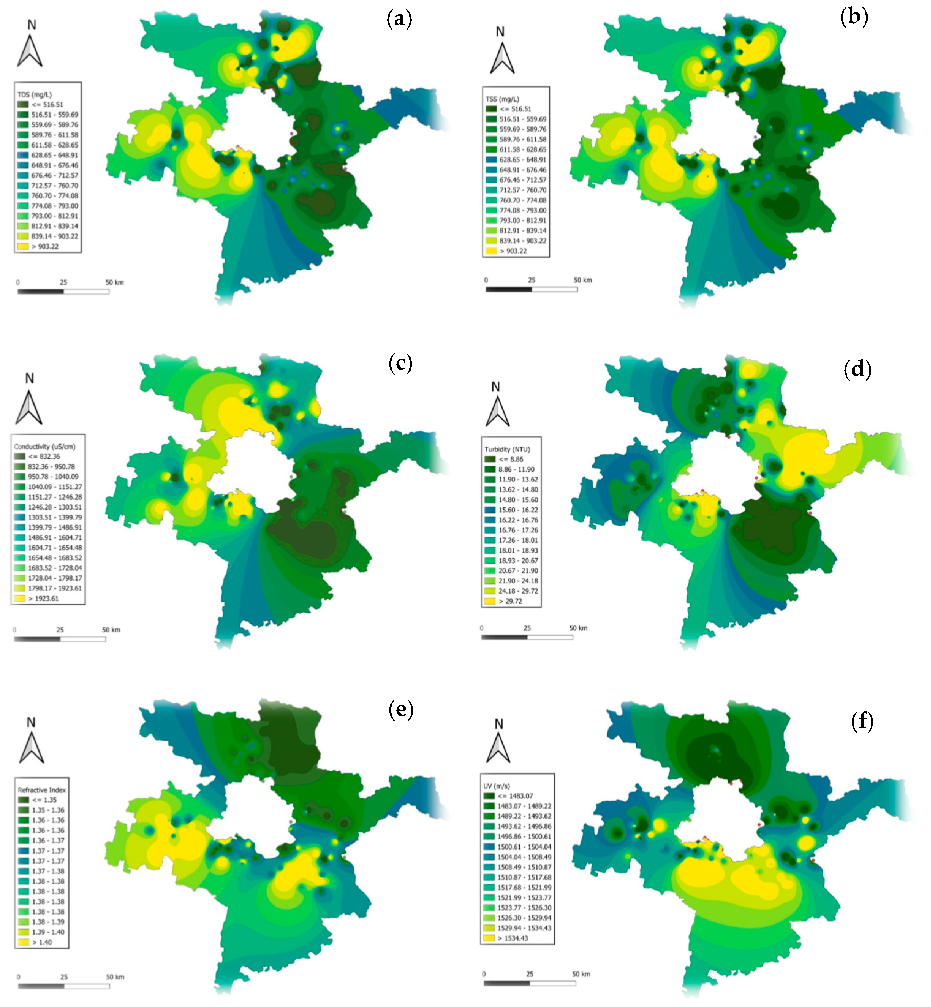
The GIS mapping of physical water quality parameters across the Delhi-surrounding districts highlights significant spatial variability, with direct implications for Delhi’s interconnected water systems (Figure 1). Total dissolved solids (TDS) and total suspended solids (TSS) exhibit higher concentrations in southern regions, exceeding 900 mg/L, due to industrial discharges and agricultural runoff, potentially impacting Delhi’s water quality through shared waterways, while northern areas show values below 600 mg/L. Conductivity also peaks in central and southern zones (>1800 µS/cm), indicating heightened ionic contamination, which may challenge Delhi’s water treatment processes. Turbidity hotspots (>25 NTU) are concentrated in southern areas, reflecting sediment and organic matter accumulation, with lower values (<10 NTU) in northern regions. The refractive index remains consistent (1.35–1.40), with slight central elevations indicating increased dissolved content, while ultrasonic velocity (1450–1550 m/s) shows minimal variation, reflecting uniformity in water density.
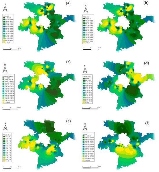
Figure 1.
GIS mapping of physical water quality parameters across Delhi–surrounding districts: (a) TDS; (b) TSS; (c) conductivity; (d) turbidity; (e) refractive index; (f) ultrasonic velocity.
4.1.2. Chemical Parameters
The GIS mapping of chemical parameters demonstrates distinct spatial patterns, highlighting their cascading impact on Delhi’s interconnected water systems. In Figure 2a, pH levels vary from acidic (<4.22) in urbanized zones to near-neutral (>7.35) in less impacted regions, with acidic zones potentially affecting Delhi’s water quality through shared surface water flows. Figure 2b highlights elevated BOD (>17.59 mg/L) near densely populated and stagnant areas, indicating significant organic pollution, which may contribute to oxygen depletion in downstream water sources connected to Delhi. Figure 2c shows critically low DO (<2.35 mg/L) in polluted regions, primarily due to organic matter decomposition and industrial effluents consuming dissolved oxygen, posing risks of hypoxia in aquatic ecosystems. Higher levels (>4.80 mg/L) are observed in well-aerated zones, particularly in areas with active water flow, offering some resilience against oxygen depletion. Figure 2d reveals high water hardness (>292.09 mg/L) in regions influenced by geological leaching and industrial activities, with potential implications for water treatment challenges in Delhi. This spatial analysis underscores the necessity of addressing upstream contamination to safeguard Delhi’s water resources.
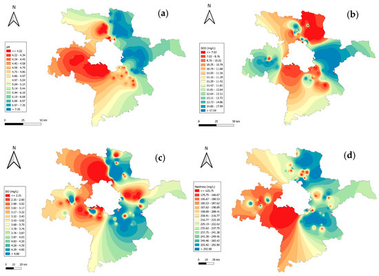
Figure 2.
GIS mapping of chemical parameters across Delhi–surrounding districts: (a) pH; (b) BOD; (c) DO; (d) hardness.
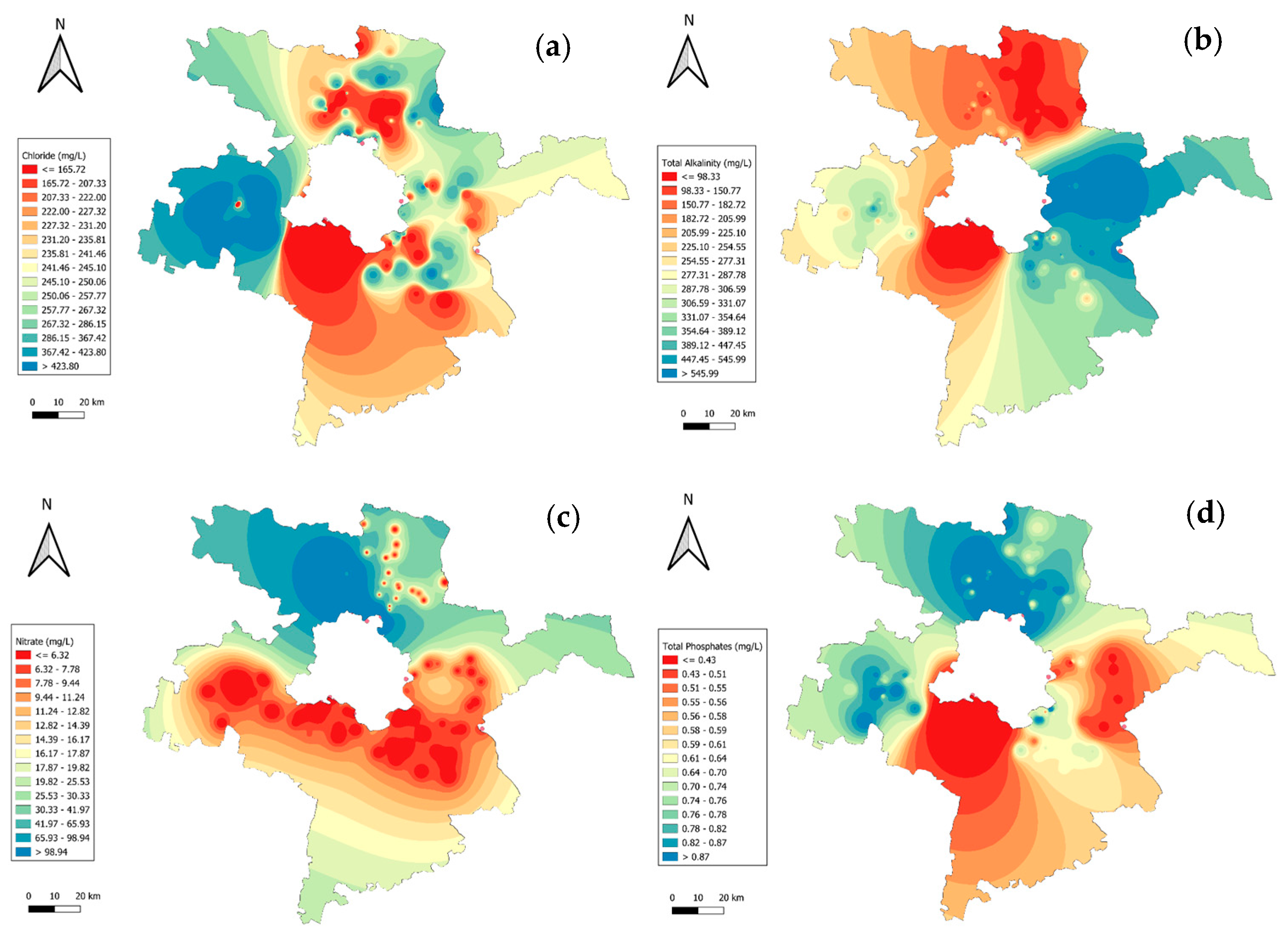
The spatial distribution of chemical parameters in Figure 3 highlights their potential downstream impact on Delhi’s water resources, emphasizing the need for focused mitigation strategies. Chloride concentrations (Figure 3a) ranged from 165.72 to 423.30 mg/L, with elevated levels in central districts, like Sonipat, potentially influencing Delhi’s shared water systems due to industrial discharge. Total alkalinity (Figure 3b) varied between 98.33 and 545.99 mg/L, with prominent values in Gurugram and Jhajjar, attributed to soil composition and agricultural runoff, affecting water usability. Nitrate levels (Figure 3c) ranged from 6.32 to 96.94 mg/L, with southern hotspots in Faridabad indicating excessive fertilizer application, raising concerns over eutrophication in interconnected water bodies. Total phosphates (Figure 3d), with values between 0.43 to 0.87 mg/L, were highest in northern and central regions, linked to wastewater inputs and agricultural activities, which may contribute to nutrient pollution in Delhi’s water sources. This analysis underscores the cascading effects of regional contamination on Delhi’s water quality.
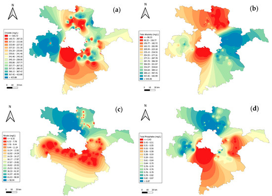
Figure 3.
GIS mapping of chemical parameters across Delhi–surrounding districts: (a) chloride; (b) total alkalinity; (c) nitrate; (d) total phosphates.
4.1.3. Microbiological Parameters
The GIS mapping of microbiological parameters reinforces the environmental implications of microbial contamination and its relevance to the fate and transport of organic pollutants in water systems. As shown in Figure 4a, total coliform concentrations exceed 1600 CFU/100 mL in urbanized zones in Faridabad, highlighting untreated sewage discharges as a significant contributor to organic pollutant loads. Lower concentrations, such as <25 CFU/100 mL observed in Chandu Budhera Canal, Gurugram, reflect localized effective wastewater management. Similarly, Figure 4b reveals fecal coliform levels surpassing 540 CFU/100 mL in urban areas of Gurugram, indicative of poor sanitation and untreated effluents, while rural areas around Delhi, report values as low as 12 CFU/100 mL. These microbial hotspots are closely associated with the transport of persistent organic pollutants (POPs), including industrial chemicals and pharmaceutical residues, as biochemical metabolisms often accelerates pollutant degradation or transformation. The microbial contamination of interconnected water systems directly impacts Delhi’s water quality, compounding the risks posed by organic pollutants.
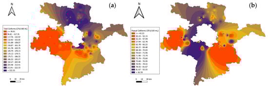
Figure 4.
Spatial distribution of microbiological parameters in Delhi–surrounding districts: (a) total coliforms; (b) fecal coliforms.
These findings emphasize the need for integrated wastewater treatment and ecological remediation strategies to address both microbial and chemical contamination, ensuring the protection of aquatic ecosystems and human health.
4.1.4. Water Quality Index
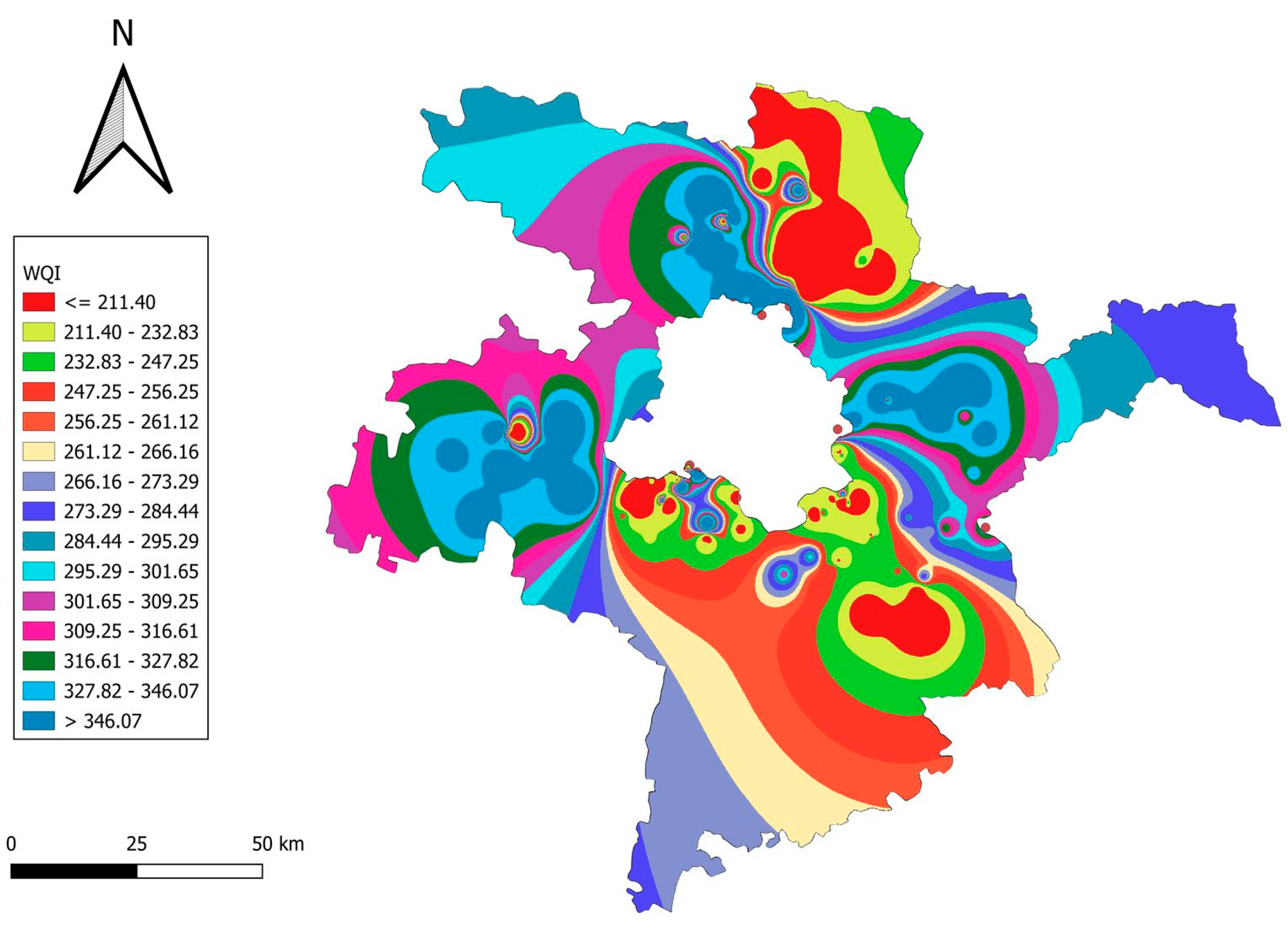
Figure 5 illustrates the spatial distribution of the WQI across districts surrounding Delhi. Industrialized regions, such as Faridabad, Gurugram, and parts of Sonipat, exhibit critically high WQI values (>600), attributed to extensive industrial discharges and untreated organic pollutants. In contrast, rural areas in other districts, like Jhajjar and Baghpat, show comparatively lower WQI values (<200), reflecting minimal anthropogenic impact. Urban hotspots within Ghaziabad and Gautam Buddh Nagar, along with central Delhi’s outskirts, record WQI values ranging between 400 and 707, highlighting the adverse effects of urbanization and insufficient wastewater management. This differentiation underscores the urgent need for targeted remediation measures to safeguard water resources and public health in both urban and peri-urban zones.
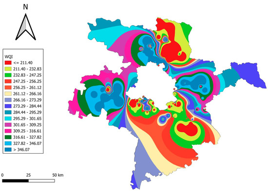
Figure 5.
Spatial distribution of water quality index (WQI) across Delhi–surrounding districts.
4.2. Machine Learning Model Performance
Water quality index (WQI) modeling plays a crucial role in identifying and mitigating environmental risks posed by pollutants in water systems. Traditional WQI calculations rely on complete experimental datasets; however, machine learning (ML) models enhance predictive capability by inferring missing values and estimating WQI in unmonitored regions. This adaptability is particularly critical for rapidly urbanizing and industrializing areas, where continuous real-time monitoring may not be feasible. By capturing complex, nonlinear relationships among water quality parameters, ML-based models enable early detection of emerging contamination risks, supporting data-driven decision-making for sustainable water resource management. This section evaluates the performance of four machine learning models, namely linear regression (LR), random forest (RF), Gaussian process regression (GPR), and support vector machines (SVMs). Their prediction capabilities, measured through correlation coefficient (CC), mean absolute error (MAE), and root mean squared error (RMSE), are discussed in detail.
4.2.1. Performance Analysis of Linear Regression (LR)
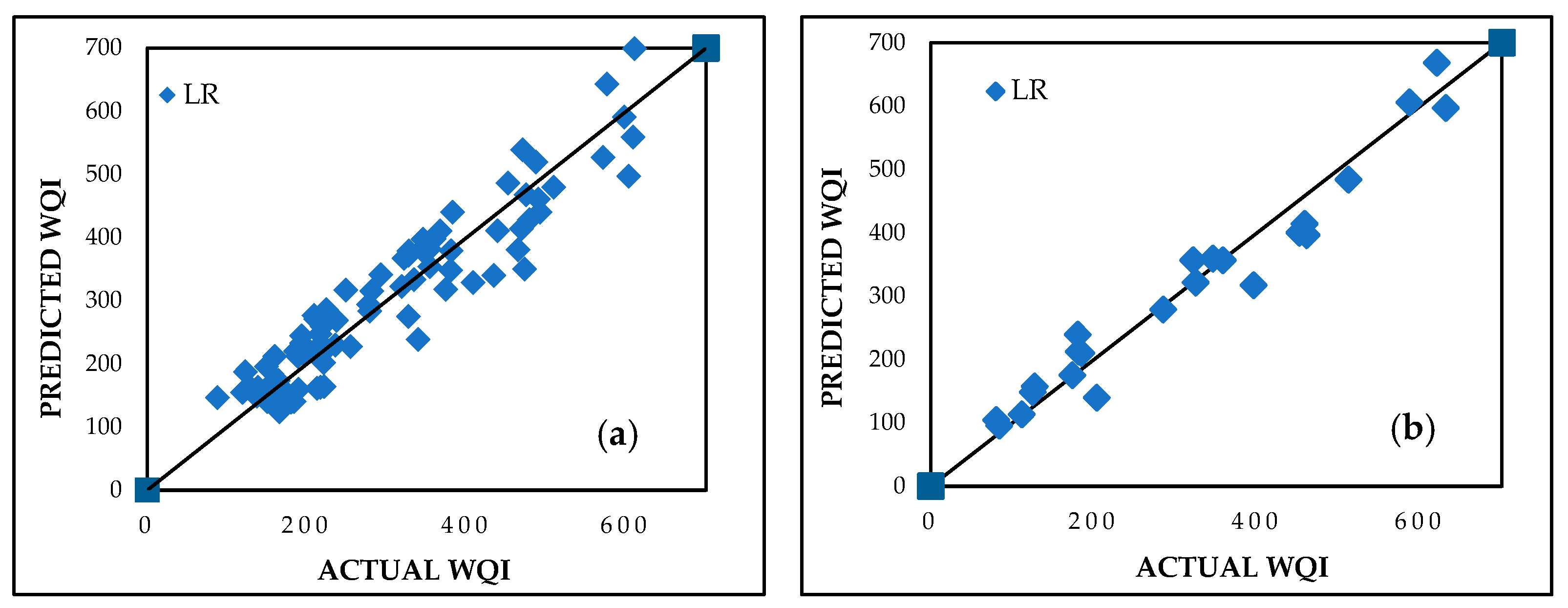
The LR model demonstrated a robust prediction capability for WQI. It was developed using the WEKA 3.8.6 software and is based on the least squares method, which minimizes the sum of squared residuals to estimate the relationship between the independent variables and WQI. The batch size was set to 100, numerical precision was maintained at two decimal places, and default settings for debugging and additional statistics were used to ensure computational efficiency and interpretability. Performance metrics included CC values of 0.9435 and 0.9791, MAE values of 39.7008 and 31.0651, and RMSE values of 48.3181 and 37.8582 for the training and testing datasets, respectively. These results, visualized in Figure 6a,b for the training and testing datasets, respectively, reflect the model’s reliability. Equation (13) presents the derived prediction equation as follows:
where S, s, C, p, B, D, N, P, T, F represent total solids, total suspended solids, conductivity, pH, biochemical oxygen demand, dissolved oxygen, nitrate, total phosphates, total coliforms, and fecal coliforms, respectively.
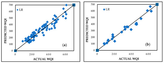
Figure 6.
Predicted vs. actual WQI performance for LR during (a) training and (b) testing stages.
4.2.2. Performance Analysis of Random Forest (RF)
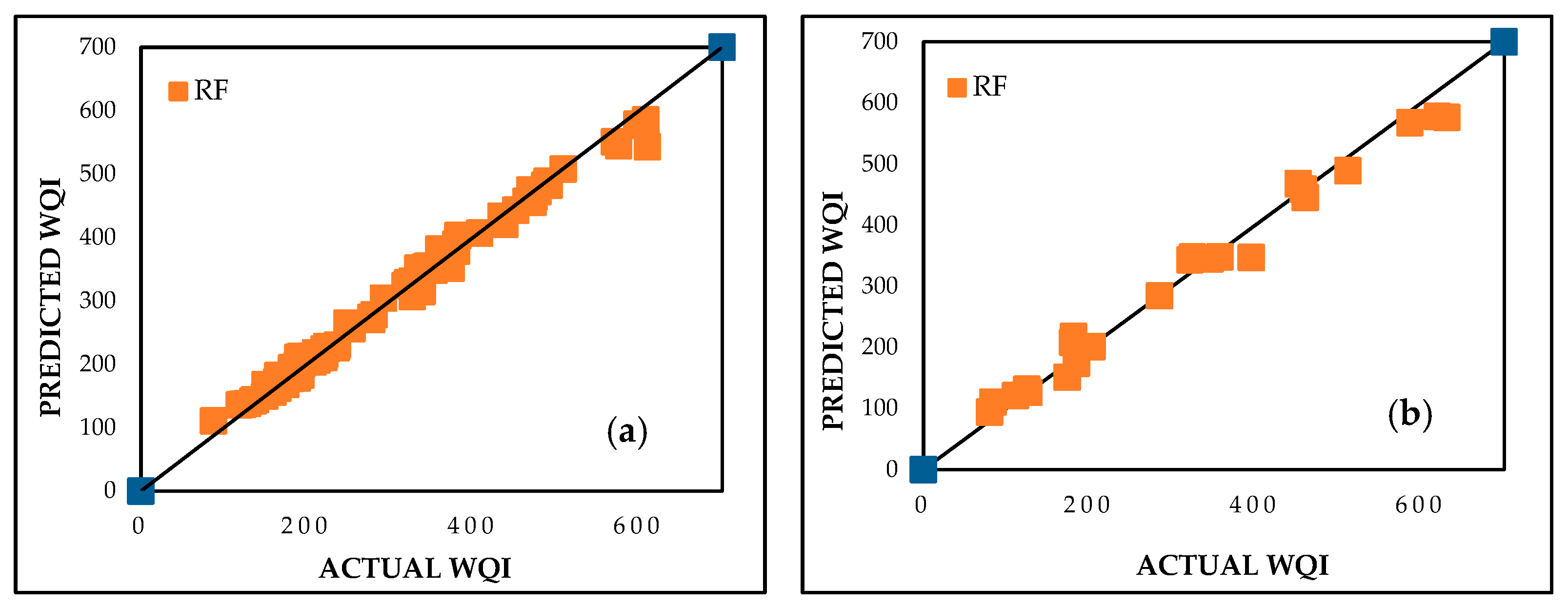
The random forest (RF) model was developed using an iterative trial-and-error process to determine the most suitable hyperparameters. The final configuration consisted of 10 decision trees (K = 10) and 1 feature per split (m = 1) to optimize computational efficiency while preventing overfitting. The RF algorithm excels in handling complex, nonlinear interactions among water quality parameters, making it particularly effective for assessing contamination trends in industrialized and urbanized regions. The RF model achieved exceptional performance with CC values of 0.9963 and 0.9925, MAE values of 10.2745 and 21.7398, and RMSE values of 15.4521 and 29.8107 for the training and testing datasets, respectively. The superior results are visualized in Figure 7. The RF model’s ability to handle nonlinear relationships makes it highly suitable for complex datasets, like WQI, highlighting contamination trends influenced by industrial discharges and urban runoff in the Delhi region.
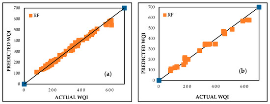
Figure 7.
Predicted vs. actual WQI performance for RF during (a) training and (b) testing stages.
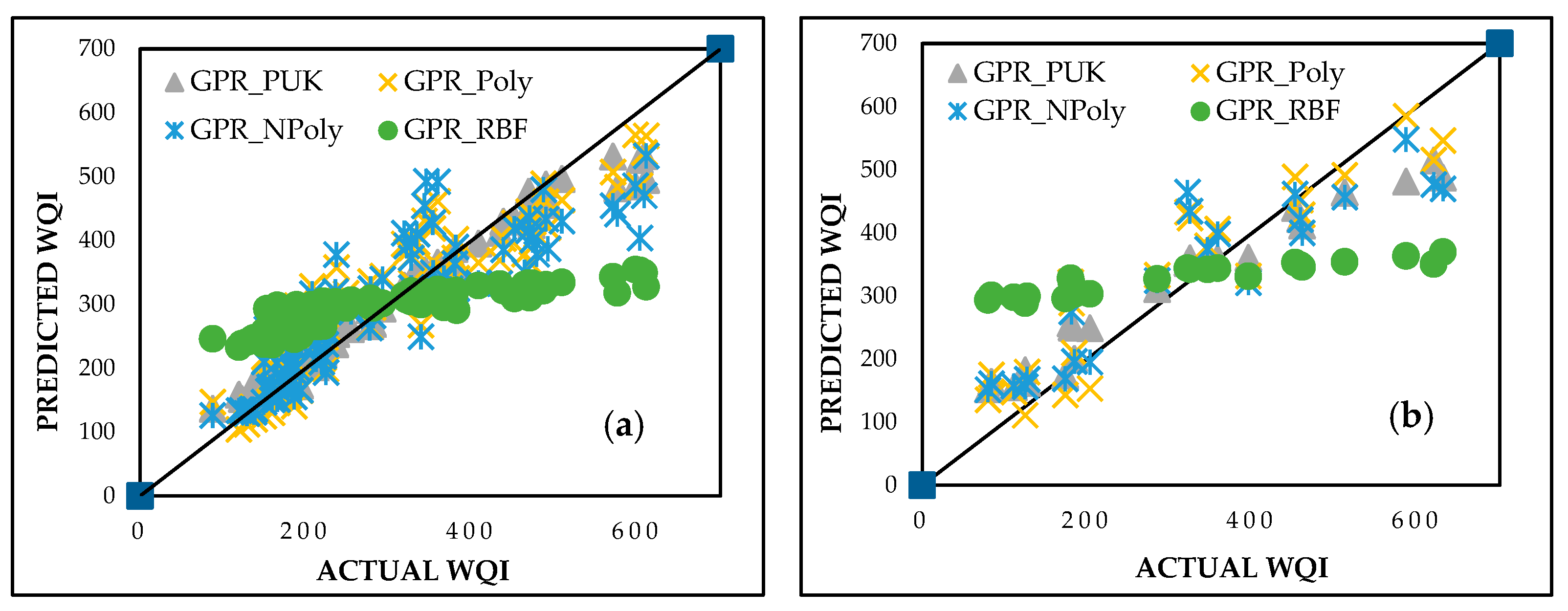
4.2.3. Performance Analysis of Gaussian Process Regression (GPR)
The GPR model was evaluated using four kernel functions, namely polynomial (GPR_Poly), normalized polynomial (GPR_NPoly), Pearson universal kernel (GPR_PUK), and radial basis function (GPR_RBF). The noise parameter was set to 0.01, with kernel-specific hyperparameters optimized for performance. The normalized polynomial kernel was configured with an exponent (d) of 1, while the polynomial kernel had an exponent (d) of 3. For the Pearson VII kernel, the scale (σ) was set to 1, and the shape parameter (ω) was adjusted to 0.1. The radial basis function kernel was applied with a gamma (γ) value of 1 to ensure accurate modeling of complex, nonlinear relationships in the dataset. Among these, GPR_PUK exhibited the best predictive capability, achieving CC values of 0.9818 and 0.9811, MAE values of 24.2197 and 54.0376, and RMSE values of 38.8481 and 68.4466 for the training and testing datasets, respectively. These results are summarized in Table 4 and visualized in Figure 8. The strong predictive accuracy of GPR_PUK highlights its effectiveness in capturing nonlinear relationships in WQI prediction.
Table 4.
Performance evaluation metrics for GPR.
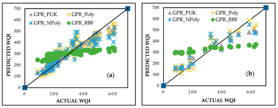
Figure 8.
Predicted vs. actual WQI performance for GPR during (a) training and (b) testing stages.
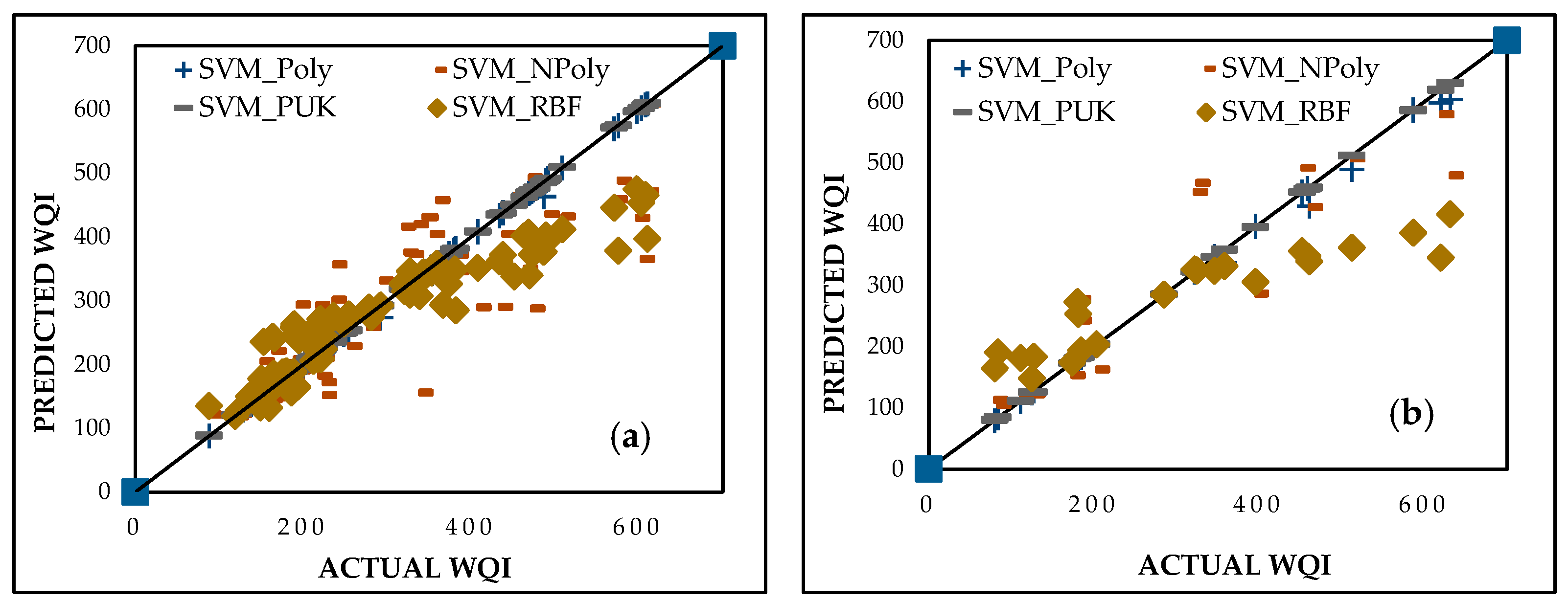
4.2.4. Performance Analysis of Support Vector Machines (SVM)
The support vector machine regression (SVMR) model was developed using four kernel functions, namely polynomial (SVM_Poly), normalized polynomial (SVM_NPoly), Pearson universal kernel (SVM_PUK), and radial basis function (SVM_RBF). The optimal regularization parameter (C) was set to 2, while all other kernel function parameters were kept consistent with those in the GPR model for fair comparisons. The SVM_Poly model outperformed the others, achieving exceptional CC values of 0.9975 and 0.9997 for the training and testing datasets, respectively. Its MAE values were 1.4494 and 5.6085 and its RMSE values were 21.7967 and 11.4158 for the respective datasets. These metrics, presented in Table 5 and visualized in Figure 9, emphasize the model’s accuracy and suitability for predicting WQI in diverse environmental conditions.
Table 5.
Performance evaluation metrics for SVM.
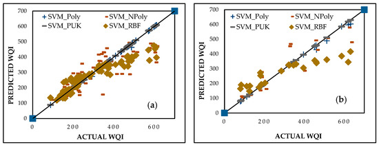
Figure 9.
Predicted vs. actual WQI performance for SVM during (a) training and (b) testing stages.
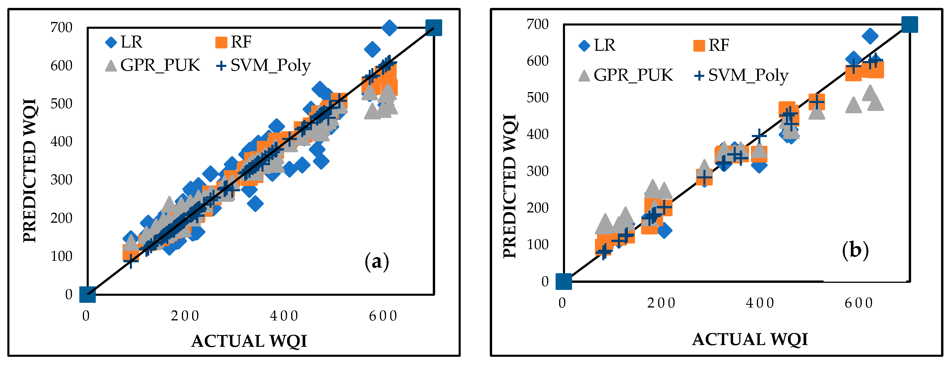
4.2.5. Assessment of Intercomparison of the LR, RF, GPR_PUK, and SVM_Poly Models
The intercomparison of machine learning models, including linear regression (LR), random forest (RF), GPR_PUK, and SVM_Poly, is summarized in Table 6. The SVM_Poly model demonstrates superior performance, achieving CC values of 0.9975 and 0.9997 for the training and testing datasets, respectively, along with the lowest MAE (1.4494 and 5.6085, respectively) and RMSE (21.7967 and 11.4158, respectively). RF follows as a strong contender, with CC values of 0.9963 and 0.9925, respectively, and a relatively low MAE (10.2745 and 21.7398, respectively) and RMSE (15.4521 and 29.8107, respectively). RF and GPR_PUK also deliver robust results, but their accuracy metrics are marginally lower than SVM_Poly. LR shows reliable performance but with higher deviations in predicted values.
Table 6.
Performance metrics of the LR, RF, GPR_PUK, and SVM_Poly models.
Figure 10a,b present the agreement plots between actual and predicted WQI values for training and testing datasets, respectively. SVM_Poly shows the closest alignment, followed by RF and GPR_PUK, while LR displays slightly higher residuals.
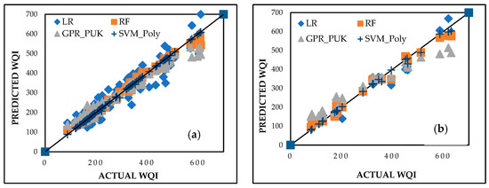
Figure 10.
Predicted vs. actual WQI performance for intercomparison models during (a) training and (b) testing stages.
This evaluation underscores the superiority of SVM_Poly in predicting WQI, ensuring precise assessments critical for managing water quality and mitigating the environmental impacts of pollutants in Delhi and surrounding regions.
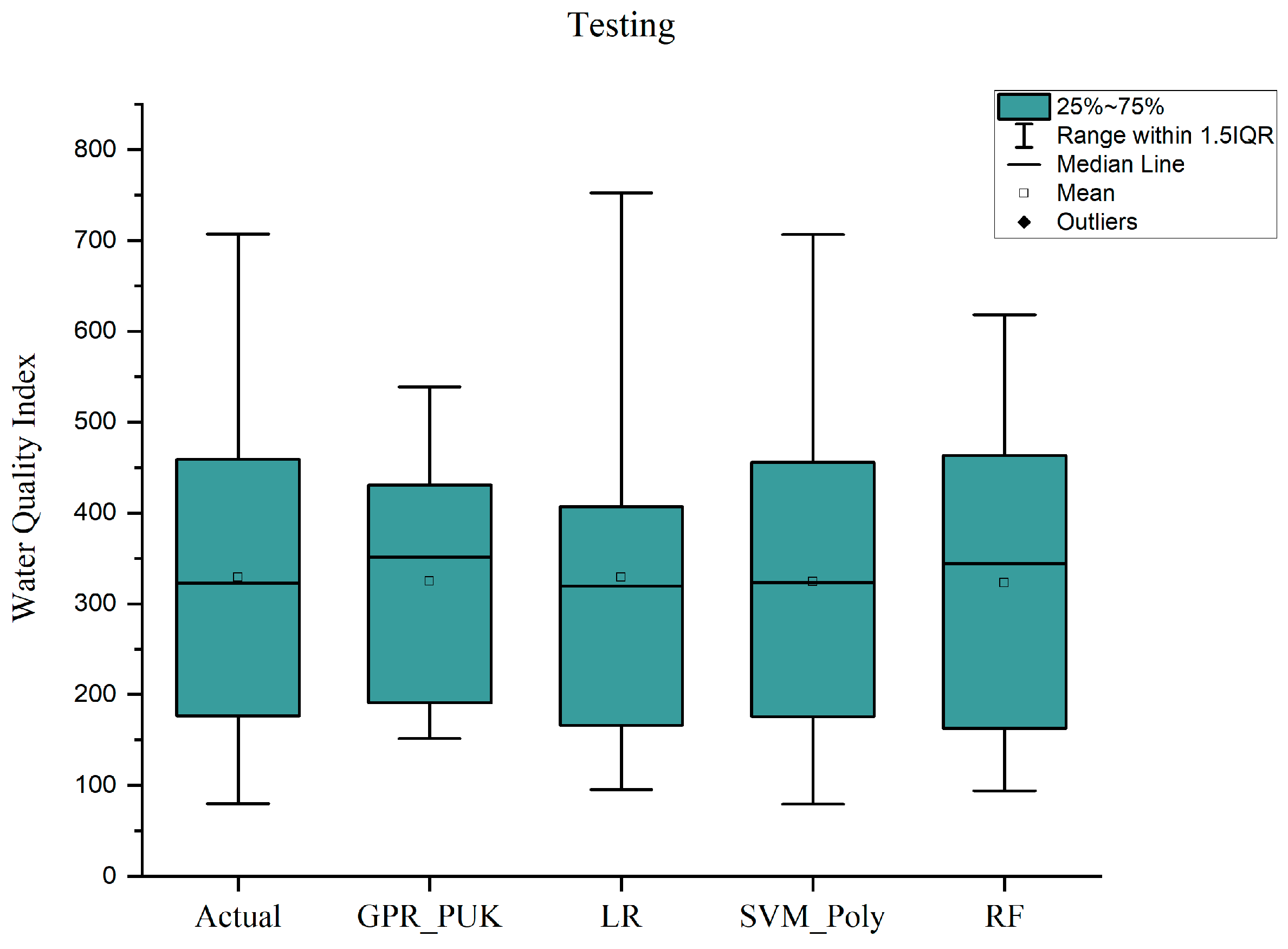
4.3. Visualization of Model Results
The box plot (Figure 11) illustrates the comparison of predicted water quality index (WQI) values across the models (GPR_PUK, LR, SVM_Poly, RF) against the actual data for the testing dataset. The interquartile range (IQR) and median line indicate the distribution of predictions. SVM_Poly demonstrates a closer alignment with the actual data, characterized by minimal variation and reduced outliers. GPR_PUK and RF exhibit slightly larger deviations, while LR shows moderate performance. The tighter range and consistent median of SVM_Poly suggest its superior predictive accuracy, reinforcing its suitability for WQI modeling.

Figure 11.
Box plot of actual vs. predicted WQI for testing dataset.
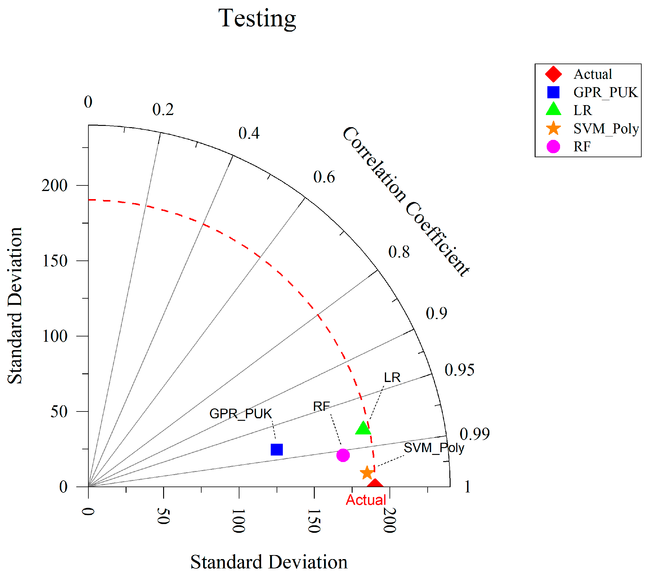
The Taylor diagram (Figure 12) provides a comprehensive evaluation of model performance by comparing correlation coefficients and standard deviations. SVM_Poly stands out with the highest correlation coefficient and minimal standard deviation, closely matching the actual dataset. GPR_PUK, while showing strong performance, exhibits slightly higher deviations. RF and LR demonstrate lower correlation coefficients and larger standard deviations compared to SVM_Poly. The diagram unequivocally identifies SVM_Poly as the most effective model for accurately predicting WQI in the testing dataset.
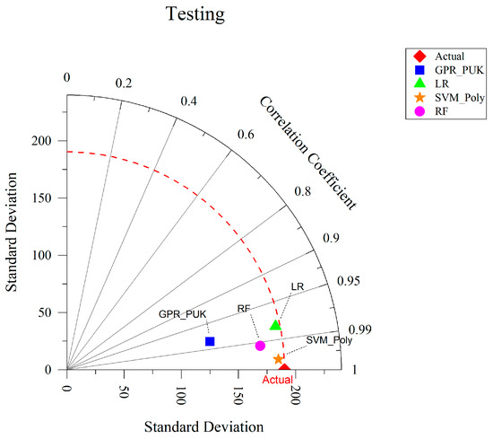
Figure 12.
Taylor’s diagram for WQI prediction performance on the testing dataset.
4.4. Sensitivity Analysis
The sensitivity analysis conducted with the SVM_Poly model identified total suspended solids as the most critical parameter influencing WQI predictions, as shown in Table 7. Its exclusion led to a sharp drop in accuracy, with CC declining to 0.6589 and significant increases in MAE (75.5624) and RMSE (130.7235). BOD emerged as the second-most influential factor, with CC reducing to 0.8112 and corresponding increases in MAE (65.4325) and RMSE (115.6527). Other parameters, like nitrate and conductivity, also contributed notably to the model’s predictive performance. In contrast, fecal coliforms and pH showed a lesser impact. These findings emphasize the importance of certain parameters, like total suspended solids and BOD, in understanding the environmental fate and transport of organic and chemical pollutants, crucial for addressing water quality challenges in urbanized regions, like Delhi-NCR.
Table 7.
Sensitivity analysis of input parameters using SVM_Poly during testing phase.
5. Conclusions
This research presents a novel methodological approach to assessing water quality in the urban–industrial confluence zones (UICZs) surrounding the National Capital Territory (NCT) of India, integrating spatial analytics with advanced machine learning. The analysis of water samples from Gautam Buddha Nagar, Ghaziabad, Faridabad, Sonipat, Gurugram, Jhajjar, and Baghpat revealed significant contamination disparities. Industrial hotspots, such as Faridabad and Gurugram, exhibited critical WQI levels exceeding 600, driven by untreated industrial discharges rich in organic and inorganic pollutants, while rural districts, like Jhajjar and Baghpat, displayed WQI levels below 200, indicative of lower anthropogenic impacts. SVM_Poly demonstrated unparalleled predictive performance with testing CC, RMSE, and MAE values of 0.9997, 11.4158, and 5.6085, respectively, making it the most suitable model for WQI prediction. RF followed, with robust metrics of 0.9925, 29.8107, and 21.7398, while GPR_PUK and LR provided reliable, albeit less accurate, predictions. Sensitivity analysis identified total suspended solids as the most influential parameter, reaffirming the necessity for targeted interventions. The integration of ML-based WQI prediction offers a scalable approach to water quality assessment, reducing dependency on exhaustive field sampling while enabling proactive identification of pollution hotspots in rapidly developing industrial zones. This study’s application of GIS and ML frameworks provides a transformative approach to understanding the fate and transport of organic and inorganic pollutants, particularly within urban–industrial contexts. The study’s integration of GIS and ML frameworks provides a transformative approach to understanding the fate and transport of organic and inorganic pollutants, particularly within urban–industrial contexts. The use of spatial interpolation techniques, such as kriging and inverse distance weighting (IDW) further enhances GIS-based WQI estimation, enabling predictions in unsampled regions and strengthening spatial decision-making in water quality management. The insights underscore the critical need for improved wastewater management and policy-driven actions to protect Delhi’s water ecosystems from escalating ecological risks. This research sets a precedent for leveraging computational models in sustainable water resource management, offering replicable methodologies for global applications.
Author Contributions
Conceptualization, B.K.S. and L.G.; methodology, B.K.S.; software, B.P. and P.S.; validation, B.K.S., B.P. and P.K.S.; formal analysis, L.G.; investigation, B.K.S. and P.K.S.; resources, B.K.S.; data curation, B.P.; writing—original draft preparation, B.K.S.; writing—review and editing, B.K.S. and P.S.; visualization, A.K.S.; supervision, B.K.S.; project administration, B.K.S.; funding acquisition, A.K.S. All authors have read and agreed to the published version of the manuscript.
Funding
This research received no external funding.
Data Availability Statement
The datasets generated during and analyzed during the current study are available from the corresponding author on reasonable request.
Conflicts of Interest
The authors declare no conflicts of interest.
References
- Zhang, Y.; Deng, J.; Qin, B.; Zhu, G.; Zhang, Y.; Jeppesen, E.; Tong, Y. Importance and vulnerability of lakes and reservoirs supporting drinking water in China. Fundam. Res. 2023, 3, 265–273. [Google Scholar] [CrossRef] [PubMed]
- Saxena, V. Water Quality, Air Pollution, and Climate Change: Investigating the Environmental Impacts of Industrialization and Urbanization. Water Air Soil Pollut. 2025, 236, 73. [Google Scholar] [CrossRef]
- Mukhopadhyay, R.; Sarkar, B.; Jat, H.S.; Sharma, P.C.; Bolan, N.S. Soil salinity under climate change: Challenges for sustainable agriculture and food security. J. Environ. Manag. 2021, 280, 111736. [Google Scholar] [CrossRef] [PubMed]
- Rangel-Buitrago, N.; Galgani, F.; Neal, W.J. Addressing the global challenge of coastal sewage pollution. Mar. Pollut. Bull. 2024, 201, 116232. [Google Scholar] [CrossRef]
- Akhtar, N.; Syakir Ishak, M.I.; Bhawani, S.A.; Umar, K. Various natural and anthropogenic factors responsible for water quality degradation: A review. Water 2021, 13, 2660. [Google Scholar] [CrossRef]
- Naz, I.; Fan, H.; Aslam, R.W.; Tariq, A.; Quddoos, A.; Sajjad, A.; Soufan, W.; Almutairi, K.F.; Ali, F. Integrated Geospatial and Geostatistical Multi-Criteria Evaluation of Urban Groundwater Quality Using Water Quality Indices. Water 2024, 16, 2549. [Google Scholar] [CrossRef]
- Kumar, S.; Sarkar, A.; Ali, S.; Shekhar, S. Groundwater system of national capital region Delhi, India. In Groundwater of South Asia; Mukherjee, A., Ed.; Springer: Singapore, 2018; Volume 1, pp. 131–152. [Google Scholar] [CrossRef]
- Shukla, B.K.; Sharma, P.K.; Yadav, H.; Singh, S.; Tyagi, K.; Yadav, Y.; Rajpoot, N.K.; Rawat, S.; Verma, S. Advanced membrane technologies for water treatment: Utilization of nanomaterials and nanoparticles in membranes fabrication. J. Nanopart. Res. 2024, 26, 222. [Google Scholar] [CrossRef]
- Dasgupta, P.; Kumar, V.; Malik, A.; Kumar, M. Wastewater treatment systems for city-based municipal drains for achieving sustainability. Circ. Econ. Sustain. 2023, 3, 585–606. [Google Scholar] [CrossRef]
- Vaid, M.; Sarma, K.; Kala, P.; Gupta, A. The plight of Najafgarh drain in NCT of Delhi, India: Assessment of the sources, statistical water quality evaluation, and fate of water pollutants. Environ. Sci. Pollut. Res. 2022, 29, 90580–90600. [Google Scholar] [CrossRef]
- Sharma, M.; Rawat, S.; Kumar, D.; Awasthi, A.; Sarkar, A.; Sidola, A.; Choudhury, T.; Kotecha, K. The state of the Yamuna River: A detailed review of water quality assessment across the entire course in India. Appl. Water Sci. 2024, 14, 175. [Google Scholar] [CrossRef]
- Gupta, N.; Yadav, S.; Chaudhary, N. Time Series Analysis and Forecasting of Water Quality Parameters along Yamuna River in Delhi. Procedia Comput. Sci. 2024, 235, 3191–3206. [Google Scholar] [CrossRef]
- Rajan, M.; Karunanidhi, D.; Jaya, J.; Preethi, B.; Subramani, T.; Aravinthasamy, P. A comprehensive review of human health hazards exposure due to groundwater contamination: A global perspective. Phys. Chem. Earth A/B/C 2024, 135, 103637. [Google Scholar] [CrossRef]
- Chowdhuri, A.; Das, B.K.; Singh, S.; Gupta, C.K. Assuaging Human Health Concerns Through Analysis of Physicochemical Parameters of Potable Water Samples in Delhi. J. Innov. Inclus. Dev. 2016, 1, 20–25. [Google Scholar]
- Khan, W.U.; Ahmed, S.; Dhoble, Y.; Madhav, S. A critical review of hazardous waste generation from textile industries and associated ecological impacts. J. Indian Chem. Soc. 2023, 100, 100829. [Google Scholar] [CrossRef]
- Mangotra, A.; Singh, S.K. Physicochemical assessment of industrial effluents of Kala Sanghian drain, Punjab, India. Environ. Monit. Assess. 2024, 196, 320. [Google Scholar] [CrossRef]
- Venkatesh, J.; Partheeban, P.; Baskaran, A.; Krishnan, D.; Sridhar, M. Wireless sensor network technology and geospatial technology for groundwater quality monitoring. J. Ind. Inf. Integr. 2024, 38, 100569. [Google Scholar] [CrossRef]
- Bohlok, D.; Mezher, M.; Houshaymi, B.; Fakhoury, M.; Khalil, M.I. Microbiological and physicochemical water quality assessments of the Upper Basin Litany River, Lebanon. Environ. Monit. Assess. 2025, 197, 74. [Google Scholar] [CrossRef]
- Shaban, J.; Al-Najar, H.; Kocadal, K.; Almghari, K.; Saygi, S. The Effect of Nitrate-Contaminated Drinking Water and Vegetables on the Prevalence of Acquired Methemoglobinemia in Beit Lahia City in Palestine. Water 2023, 15, 1989. [Google Scholar] [CrossRef]
- Zhang, P.; Liu, J.; Yang, F.; Xie, S.; Wei, C. Effects of Phosphate and Arsenate on As Metabolism in Microcystis aeruginosa at Different Growth Phases. Water 2024, 16, 940. [Google Scholar] [CrossRef]
- Effendi, H.; Wardiatno, Y. Water quality status of Ciambulawung River, Banten Province, based on pollution index and NSF-WQI. Procedia Environ. Sci. 2015, 24, 228–237. [Google Scholar] [CrossRef]
- Nyenje, P.M.; Foppen, J.W.; Uhlenbrook, S.; Kulabako, R.; Muwanga, A. Eutrophication and nutrient release in urban areas of sub-Saharan Africa—A review. Sci. Total Environ. 2010, 408, 447–455. [Google Scholar] [CrossRef] [PubMed]
- Affum, A.O.; Osae, S.D.; Nyarko, B.J.B.; Afful, S.; Fianko, J.R.; Akiti, T.T.; Adomako, D.; Acquaah, S.O.; Dorleku, M.; Antoh, E.; et al. Total coliforms, arsenic and cadmium exposure through drinking water in the Western Region of Ghana: Application of multivariate statistical technique to groundwater quality. Environ. Monit. Assess. 2015, 187, 1. [Google Scholar] [CrossRef] [PubMed]
- Kamizoulis, G.; Saliba, L. Development of coastal recreational water quality standards in the Mediterranean. Environ. Int. 2004, 30, 841–854. [Google Scholar] [CrossRef] [PubMed]
- Ibangha, I.A.I.; Madueke, S.N.; Akachukwu, S.O.; Onyeiwu, S.C.; Enemuor, S.C.; Chigor, V.N. Physicochemical and bacteriological assessment of Wupa wastewater treatment plant effluent and the effluent-receiving Wupa River in Abuja, Nigeria. Environ. Monit. Assess. 2024, 196, 30. [Google Scholar] [CrossRef]
- Pluym, T.; Waegenaar, F.; De Gusseme, B.; Boon, N. Microbial drinking water monitoring now and in the future. Microb. Biotechnol. 2024, 17, e14532. [Google Scholar] [CrossRef]
- Kefi, M.; Aden, M.M.; Ali, B.B. Water Quality Monitoring for Irrigation by the Integration of Water Quality Index in a Geographic Information System Environment in Chiba Watershed, Nabeul, Tunisia. Water Conserv. Sci. Eng. 2024, 9, 20. [Google Scholar] [CrossRef]
- Gomaa, H.E.; Charni, M.; Alotibi, A.A.; AlMarri, A.H.; Gomaa, F.A. Spatial distribution and hydrogeochemical factors influencing the occurrence of total Coliform and E. coli bacteria in groundwater in a hyperarid area, Ad-Dawadmi, Saudi Arabia. Water 2022, 14, 3471. [Google Scholar] [CrossRef]
- Uddin, M.G.; Nash, S.; Rahman, A.; Olbert, A.I. A comprehensive method for improvement of water quality index (WQI) models for coastal water quality assessment. Water Res. 2022, 219, 118532. [Google Scholar] [CrossRef]
- Kumar, A.; Bojjagani, S.; Maurya, A.; Kisku, G.C. Spatial distribution of physicochemical-bacteriological parametric quality and water quality index of Gomti River, India. Environ. Monit. Assess. 2022, 194, 159. [Google Scholar] [CrossRef]
- Singh, S.; Das, A.; Sharma, P. Predictive modeling of water quality index (WQI) classes in Indian rivers: Insights from the application of multiple Machine Learning (ML) models on a decennial dataset. Stoch. Environ. Res. Risk Assess. 2024, 38, 3221–3238. [Google Scholar] [CrossRef]
- Pandya, H.; Jaiswal, K.; Shah, M. A comprehensive review of machine learning algorithms and its application in groundwater quality prediction. Arch. Comput. Methods Eng. 2024, 31, 4633–4654. [Google Scholar] [CrossRef]
- Palani, S.; Liong, S.Y.; Tkalich, P. An ANN application for water quality forecasting. Mar. Pollut. Bull. 2008, 56, 1586–1597. [Google Scholar] [CrossRef]
- Asadollah, S.B.H.S.; Sharafati, A.; Motta, D.; Yaseen, Z.M. River water quality index prediction and uncertainty analysis: A comparative study of machine learning models. J. Environ. Chem. Eng. 2021, 9, 104599. [Google Scholar] [CrossRef]
- Pande, C.B.; Sidek, L.M.; Varade, A.M.; Elkhrachy, I.; Radwan, N.; Tolche, A.D.; Elbeltagi, A. Forecasting of meteorological drought using ensemble and machine learning models. Environ. Sci. Eur. 2024, 36, 160. [Google Scholar] [CrossRef]
- Weng, M.; Zhang, X.; Li, P.; Liu, H.; Liu, Q.; Wang, Y. Exploring the Impact of Land Use Scales on Water Quality Based on the Random Forest Model: A Case Study of the Shaying River Basin, China. Water 2024, 16, 420. [Google Scholar] [CrossRef]
- Zeng, J.; Nakanishi, T.; Itoh, S. Two-year Monitoring of Microbiological Water Quality in Small Water Supply Systems: Implications for Microbial Risk Management. Environ. Manag. 2024, 74, 256–267. [Google Scholar] [CrossRef]
- Drogkoula, M.; Kokkinos, K.; Samaras, N. A comprehensive survey of machine learning methodologies with emphasis in water resources management. Appl. Sci. 2023, 13, 12147. [Google Scholar] [CrossRef]
- Kumar, M.; Herbert, R.; Jha, P.K.; Deka, J.P.; Rao, M.S.; Ramanathan, A.L.; Kumar, B. Understanding the seasonal dynamics of the groundwater hydrogeochemistry in National Capital Territory (NCT) of India through geochemical modelling. Aquat. Geochem. 2016, 22, 211–224. [Google Scholar] [CrossRef]
- Chowdary, V.M.; Rao, N.H.; Sarma, P.B.S. Decision support framework for assessment of non-point-source pollution of groundwater in large irrigation projects. Agric. Water Manag. 2005, 75, 194–225. [Google Scholar] [CrossRef]
- Chinnakkaruppan, K.; Krishnamoorthy, K.; Agniraj, S. A novel predictive analysis approach for forecasting and classifying surface water data using AWQI standards and machine learning-based rule induction. Earth Sci. Inform. 2025, 18, 130. [Google Scholar] [CrossRef]
- IS 3025 (Part 16); Methods for Determination of Total Dissolved Solids. Bureau of Indian Standards: New Delhi, India, 1984.
- IS 3025 (Part 15); Methods for Determination of Total Solids. Bureau of Indian Standards: New Delhi, India, 1984.
- IS 3025 (Part 17); Methods for Determination of Suspended Solids. Bureau of Indian Standards: New Delhi, India, 1984.
- IS 3025 (Part 14); Methods for Determination of Conductivity. Bureau of Indian Standards: New Delhi, India, 1984.
- IS 3025 (Part 10); Methods for Turbidity Measurement. Bureau of Indian Standards: New Delhi, India, 1984.
- ASTM D1218-12; Standard Test Method for Refractive Index. ASTM International: West Conshohocken, PA, USA, 2012.
- ASTM E494-15; Standard Practice for Measuring Ultrasonic Velocity in Materials. ASTM International: West Conshohocken, PA, USA, 2015.
- IS 3025 (Part 11); Methods for Determination of pH Value. Bureau of Indian Standards: New Delhi, India, 1983.
- IS 3025 (Part 44); Methods for Determination of Biochemical Oxygen Demand. Bureau of Indian Standards: New Delhi, India, 1993.
- IS 3025 (Part 58); Methods for Determination of Chemical Oxygen Demand. Bureau of Indian Standards: New Delhi, India, 2006.
- IS 3025 (Part 38); Methods for Determination of Dissolved Oxygen. Bureau of Indian Standards: New Delhi, India, 1989.
- IS 3025 (Part 21); Methods for Determination of Hardness. Bureau of Indian Standards: New Delhi, India, 1983.
- IS 3025 (Part 32); Methods for Determination of Chloride. Bureau of Indian Standards: New Delhi, India, 1988.
- IS 3025 (Part 23); Methods for Determination of Alkalinity. Bureau of Indian Standards: New Delhi, India, 1986.
- IS 3025 (Part 34); Methods for Determination of Nitrate. Bureau of Indian Standards: New Delhi, India, 1988.
- IS 3025 (Part 31); Methods for Determination of Phosphates. Bureau of Indian Standards: New Delhi, India, 1988.
- IS 1622; Methods of Sampling and Microbiological Examination of Water. Bureau of Indian Standards: New Delhi, India, 1981.
- Shukla, B.K.; Teeli, M.A.; Shukla, S.K.; Chandra, R.; Bharti, N.; Singh, U. A Comprehensive Overview of Vital Water Quality Parameters. Lect. Notes Civ. Eng. 2024, 439, 1–20. [Google Scholar] [CrossRef]
- Shanmugam, N.S.; Chen, S.E.; Tang, W.; Chavan, V.S.; Diemer, J.; Allan, C.; Shukla, T.; Chen, T.; Slocum, Z.; Janardhanam, R. Spatial Interpolation of Bridge Scour Point Cloud Data Using Ordinary Kriging Method. J. Perform. Constr. Facil. 2025, 39, 06024002. [Google Scholar] [CrossRef]
- Kuttimani, R.; Raviraj, A.; Pandian, B.J.; Kar, G. Determination of water quality index in coastal area (Nagapattinam) of Tamil Nadu, India. Chem. Sci. Rev. Lett. 2017, 6, 2208–2221. [Google Scholar]
- Bıyık, E.; Huynh, N.; Kochenderfer, M.J.; Sadigh, D. Active preference-based Gaussian process regression for reward learning and optimization. Int. J. Robot. Res. 2024, 43, 665–684. [Google Scholar] [CrossRef]
- Fooladi, M.; Nikoo, M.R.; Mirghafari, R.; Madramootoo, C.A.; Al-Rawas, G.; Nazari, R. Robust clustering-based hybrid technique enabling reliable reservoir water quality prediction with uncertainty quantification and spatial analysis. J. Environ. Manag. 2024, 362, 121259. [Google Scholar] [CrossRef]
- Piccialli, V.; Schwiddessen, J.; Sudoso, A.M. Optimization meets machine learning: An exact algorithm for semi-supervised support vector machines. Math. Program. 2024, 1–43. [Google Scholar] [CrossRef]
- Reza, M.S.; Hafsha, U.; Amin, R.; Yasmin, R.; Ruhi, S. Improving SVM performance for type II diabetes prediction with an improved non-linear kernel: Insights from the PIMA dataset. Comput. Methods Programs Biomed. Update 2023, 4, 100118. [Google Scholar] [CrossRef]
- Antoniadis, A.; Lambert-Lacroix, S.; Poggi, J.M. Random forests for global sensitivity analysis: A selective review. Reliab. Eng. Syst. Saf. 2021, 206, 107312. [Google Scholar] [CrossRef]
- Ahmed, W.; Ali, K.; Zaman, S.; Raza, A. Molecular insights into anti-alzheimer’s drugs through predictive modeling using linear regression and QSPR analysis. Mod. Phys. Lett. B 2024, 38, 2450260. [Google Scholar] [CrossRef]


Disclaimer/Publisher’s Note: The statements, opinions and data contained in all publications are solely those of the individual author(s) and contributor(s) and not of MDPI and/or the editor(s). MDPI and/or the editor(s) disclaim responsibility for any injury to people or property resulting from any ideas, methods, instructions or products referred to in the content. |
© 2025 by the authors. Licensee MDPI, Basel, Switzerland. This article is an open access article distributed under the terms and conditions of the Creative Commons Attribution (CC BY) license (https://creativecommons.org/licenses/by/4.0/).