A Numerical Simulation Study of Complex Multi-Source Groundwater Based on PKAN

Abstract

Groundwater flow problems involve complex nonlinear and spatiotemporal characteristics, where traditional numerical methods (e.g., finite element, finite difference) often encounter challenges such as low computational efficiency and insufficient accuracy when dealing with complex boundary conditions and heterogeneous media. To address these issues, this study proposes a novel physics-informed Kolmogorov–Arnold network (PKAN) framework that combines the unique variable decomposition mechanism of KAN networks with physical constraints. The framework introduces three key innovations: (1) implementing KAN network’s univariate function decomposition to enhance the network’s ability to express nonlinear features; (2) designing a pre-training network mechanism to effectively handle complex boundary conditions; and (3) innovatively incorporating a distance function to achieve natural transition from boundary to interior solutions. The results demonstrate that in one-dimensional heterogeneous medium transient simulation, PKAN achieves superior prediction accuracy (R² = 0.9966, RMSE = 0.0313) compared to traditional PINN (R² = −0.7194, RMSE = 0.7001). In two-dimensional multi-well pumping system simulations, PKAN (R² = 0.917, RMSE = 0.077) similarly exhibits exceptional performance (PINN: R² = −0.3043, RMSE = 0.3067). Notably, in handling local strong gradient problems, PKAN accurately captures cone of depression characteristics and precisely reproduces inter-well interference effects, with maximum error only one-fourth that of traditional PINN. Sensitivity analysis reveals that a configuration of 50 × 50 uniform sampling points combined with four hidden layers and 64 neurons per layer achieves optimal balance between computational efficiency and simulation accuracy. These findings demonstrate PKAN’s breakthrough in groundwater numerical simulation, offering a novel approach for the efficient solution of complex hydrogeological problems.

1. Introduction

Groundwater flow problems typically involve nonlinear, spatiotemporal equations requiring precise descriptions of physical quantities such as hydraulic head and flow rates across space and time. While classical groundwater flow equations effectively capture core flow characteristics, analytical solutions are often unattainable due to complex hydrogeological conditions and uncertainties. Consequently, researchers rely on numerical methods to obtain approximate solutions. Traditional numerical approaches like Finite Element Method (FEM), Finite Difference Method (FDM), and Finite Volume Method (FVM) have been widely applied in groundwater simulation, supporting numerous engineering applications across various physical scenarios [1,2,3]. However, as groundwater simulation problems become increasingly complex, traditional numerical methods face challenges [3,4,5,6], particularly in handling complex boundary conditions, heterogeneous media, and extraction wells, often encountering issues with computational intensity, poor convergence, and limited accuracy. Furthermore, these methods typically depend on extensive grid discretization, where mesh quality significantly impacts numerical solution accuracy and convergence, especially in complex geometric or multi-scale problems, limiting their practical engineering applications.

Recent years have witnessed rapid advancement in deep learning and artificial intelligence, with physics-informed neural networks (PINN) gaining substantial attention in scientific computing [7]. PINN incorporates physical equations into neural network loss functions, enabling solution learning without extensive labeled data. This approach not only avoids traditional discretization errors but also effectively handles nonlinear problems and complex boundary conditions through neural networks’ strong approximation capabilities [8]. By directly embedding partial differential equations and boundary conditions into the loss function, the training process automatically satisfies these physical constraints, efficiently handling high-dimensional problems (e.g., time-space joint simulation) [9].

PINN has demonstrated superiority across multiple applications [10,11], particularly in complex scenario simulation. Mahmoudabadbozchelou [12] investigated PINN’s performance in various complex fluids with different non-Newtonian constitutive models; Liu [13] proposed a hard–soft physics-informed neural network (HS-PINN) to simulate pressure fluctuations around production wells; and Wang [14] developed a two-dimensional transient bioheat model based on PINN to study temperature rise induced by ultrasonic propagation. However, traditional PINN faces challenges [15] in groundwater flow simulation: firstly, while the fully connected neural network (MLP) excels in handling nonlinear problems, it lacks sufficient interpretability when dealing with physically informed groundwater flow problems, often struggling with solution accuracy and stability; secondly, PINN’s loss function depends on physical equation residuals, potentially leading to convergence issues when handling complex source-sink terms and time-varying problems [16]. Despite existing optimization measures like hard constraints and multi-region solutions, significant limitations persist in handling complex scenarios. Recent studies have highlighted the importance of properly characterizing the spatial variability of hydraulic conductivity across different scales when modeling groundwater flow, particularly in heterogeneous aquifers subject to pumping. Brunetti et al. demonstrated that the spatial variability of aquifers’ hydraulic properties can be satisfactorily described through scaling laws, which enable relating small (laboratory) scales to larger (formation/regional) ones [17]. Their experimental investigation revealed how heterogeneity enhances with increasing scale of observation. Similarly, Severino et al. provided a comprehensive analysis of the correlation structure of steady well-type flows through heterogeneous porous media, showing that the variance of hydraulic conductivity significantly influences the spatial distribution of hydraulic head, especially near pumping wells [18]. These studies emphasize that accurately modeling the degree of heterogeneity (variance of lnK) and appropriately selecting the reference scale are critical factors when simulating groundwater flow under pumping conditions. These studies emphasize that accurately modeling the degree of heterogeneity (variance of lnK) and appropriately selecting the reference scale are critical factors when simulating groundwater flow under pumping conditions. These complex spatial heterogeneity characteristics undoubtedly increase the difficulty of traditional numerical modeling approaches, including PINN.

Neural network architectures based on the Kolmogorov–Arnold theorem (KAN) have garnered attention for their unique advantages [19]. KAN networks construct powerful and interpretable activation functions by decomposing multivariate functions into linear combinations of univariate functions. This design enhances network fitting capability while addressing the interpretability limitations of traditional multilayer perceptrons (MLP) [20]. Research indicates KAN networks demonstrate superior adaptability and accuracy compared to traditional neural network architectures in complex numerical simulation tasks, particularly in solving complex partial differential equations [21].

Based on these developments, this paper introduces a novel neural network architecture—PKAN. This method enhances the traditional physics-informed neural network (PINN) structure and incorporates pre-training network mechanisms to accommodate complex boundary conditions and nonlinear characteristics in groundwater simulation. PKAN retains KAN networks’ efficient expression capabilities while improving simulation physical consistency and computational efficiency through physical prior information and constraint mechanisms. The paper’s main contribution lies in innovatively applying KAN networks to groundwater numerical simulation and designing a PKAN architecture suitable for complex groundwater flow problems. Through testing various complex scenarios, PKAN achieves high-precision simulation of groundwater head distribution without labeled data. Compared to traditional PINN, PKAN demonstrates significant performance advantages, particularly in simulation accuracy, stability, and adaptability to complex scenarios, providing robust technical support and scientific guidance for groundwater simulation.

2. Methods and Cases

2.1. Methods

The KAN network is a type of neural network based on the Kolmogorov–Arnold representation theorem [22,23,24], which proves that any multivariate continuous function can be decomposed into a combination of single-variable functions and addition operations, which can be expressed mathematically as the following:

$$\mathsf{\psi }({\mathrm{x}}_1,\dots ,{\mathrm{x}}_{\mathrm{d}})={\sum }_{\mathrm{q}=1}^{2\mathrm{d}+1}{\mathsf{\Phi }}_{\mathrm{q}}({\sum }_{\mathrm{p}=1}^{\mathrm{d}}{\mathsf{\varphi }}_{\mathrm{q},\mathrm{p}}({\mathsf{\zeta }}_{\mathrm{p}}))$$

(1)

where the function ${\mathsf{\varphi }}_{\mathrm{q},\mathrm{p}}$ is a univariate function used to map each input ${\mathsf{\zeta }}_{\mathrm{p}}$ so that ${\mathsf{\varphi }}_{\mathrm{q},\mathrm{p}}:[0,1]\to \mathrm{R}$, and ${\mathsf{\varphi }}_{\mathrm{q}}:\mathrm{R}\to \mathrm{R}$ is used for further transformation.

In KAN, a KAN layer is defined by a collection of univariate functions:

$$\mathsf{\Phi }=\{{\mathsf{\varphi }}_{\mathrm{q},\mathrm{p}}\},\mathrm{p}=1,2,\dots ,{\mathrm{n}}_{\mathrm{i}\mathrm{n}},\mathrm{q}=1,2,\dots ,{\mathrm{n}}_{\mathrm{o}\mathrm{u}\mathrm{t}}$$

(2)

The KAN architecture is viewed as a deep multi-layer structure, where each layer consists of neurons that perform linear transformations followed by nonlinear activations. For an input vector ζ, the network’s output is calculated through a series of combinations, written as follows:

$$\mathrm{K}\mathrm{A}\mathrm{N}\left(\mathsf{\zeta }\right)=({\mathsf{\Phi }}_{\mathrm{L}-1}\circ {\mathsf{\Phi }}_{\mathrm{L}-2}\circ \cdots \circ {\mathsf{\Phi }}_0)\mathsf{\zeta }$$

(3)

where L represents the total number of layers in the network.

In addition, unlike MLP, a distinctive feature of KAN is the use of a specialized activation function, which can be expressed as follows:

$$\mathsf{\varphi }\left(\mathsf{\zeta }\right)={\mathrm{w}}_{\mathrm{b}}\mathrm{b}\left(\mathsf{\zeta }\right)+{\mathrm{w}}_{\mathrm{s}}\mathrm{s}\mathrm{p}\mathrm{l}\mathrm{i}\mathrm{n}\mathrm{e}\left(\mathsf{\zeta }\right)$$

(4)

Among them, $\mathrm{b}(\mathsf{\zeta })={\displaystyle \frac{\mathsf{\zeta }}{1+\exp (-\mathsf{\zeta })}}$ is a sigmoid-like function [25], and $\mathrm{s}\mathrm{p}\mathrm{l}\mathrm{i}\mathrm{n}\mathrm{e}(\mathsf{\zeta })={\sum }_{\mathrm{i}=0}^{\mathrm{k}}{\mathrm{c}}_{\mathrm{i}}{\mathrm{B}}_{\mathrm{i}}(\mathsf{\zeta })$ is a combination of B-spline basis functions ${\mathrm{B}}_{\mathrm{i}}\left(\mathsf{\zeta }\right)$, which are polynomials of a specific degree, where ${\mathrm{c}}_{\mathrm{i}}$, ${\mathrm{w}}_{\mathrm{b}}$, and ${\mathrm{w}}_{\mathrm{s}}$ are all trainable parameters [26].

The hierarchical structure of KAN enables the network to naturally capture the multi-scale features in physical problems, which provides a theoretical basis for constructing the structure of physical information neural networks. In order to improve the network’s expressive power, the KAN network first needs to transform the input:

$${\mathsf{\zeta }}_{\mathrm{p}}^1={\mathrm{T}}_{\mathrm{p}}(\mathrm{t},\mathrm{x})={\mathrm{w}}_{\mathrm{p}}^{\mathrm{t}}\mathrm{t}+{\mathrm{w}}_{\mathrm{p}}^{\mathrm{x}}\mathrm{x}+{\mathrm{b}}_{\mathrm{p}},\mathrm{p}=1,\dots ,\mathrm{d}$$

(5)

where ${\mathrm{T}}_{\mathrm{p}}$ is a learnable affine transformation.

For the lth layer (l = 2, …, L − 1), the input–output relationship is as follows:

$${\mathsf{\zeta }}_{\mathrm{p}}^{\mathrm{l}}={\sum }_{\mathrm{q}=1}^{2\mathrm{d}+1}{\mathsf{\Phi }}_{\mathrm{q}}^{\mathrm{l}-1}({\sum }_{\mathrm{p}=1}^{\mathrm{d}}{\mathsf{\varphi }}_{\mathrm{q},\mathrm{p}}^{\mathrm{l}-1}({\mathsf{\zeta }}_{\mathrm{p}}^{\mathrm{l}-1}))$$

(6)

The univariate function ${\mathsf{\varphi }}_{\mathrm{q},\mathrm{p}}^{\mathrm{l}}$ of each layer uses a composite activation function:

$${\mathsf{\varphi }}_{\mathrm{q},\mathrm{p}}^{\mathrm{l}}(\mathsf{\zeta })={\mathrm{w}}_{\mathrm{b}}^{\mathrm{l}}{\mathrm{b}}^{\mathrm{l}}(\mathsf{\zeta })+{\mathrm{w}}_{\mathrm{s}}^{\mathrm{l}}{\mathrm{s}\mathrm{p}\mathrm{l}\mathrm{i}\mathrm{n}\mathrm{e}}^{\mathrm{l}}(\mathsf{\zeta })+{\mathrm{w}}_{\mathrm{r}}^{\mathrm{l}}{\mathrm{r}\mathrm{a}\mathrm{t}\mathrm{i}\mathrm{o}\mathrm{n}\mathrm{a}\mathrm{l}}^{\mathrm{l}}(\mathsf{\zeta })+{\mathrm{w}}_{\mathrm{f}}^{\mathrm{l}}{\mathrm{f}\mathrm{o}\mathrm{u}\mathrm{r}\mathrm{i}\mathrm{e}\mathrm{r}}^{\mathrm{l}}(\mathsf{\zeta })$$

(7)

Each item can be expressed as follows:

$${\mathrm{b}}^{\mathrm{l}}(\mathsf{\zeta })={\mathsf{\alpha }}^{\mathrm{l}}\mathsf{\zeta }\cdot \mathsf{\sigma }({\mathsf{\beta }}^{\mathrm{l}}\mathsf{\zeta })$$

(8)

$${\mathrm{s}\mathrm{p}\mathrm{l}\mathrm{i}\mathrm{n}\mathrm{e}}^{\mathrm{l}}(\mathsf{\zeta })={\sum }_{\mathrm{i}=0}^{\mathrm{k}}{\mathrm{c}}_{\mathrm{i}}^{\mathrm{l}}{\mathrm{B}}_{\mathrm{i}}^{\mathrm{l}}(\mathsf{\zeta })$$

(9)

$${\mathrm{r}\mathrm{a}\mathrm{t}\mathrm{i}\mathrm{o}\mathrm{n}\mathrm{a}\mathrm{l}}^{\mathrm{l}}(\mathsf{\zeta })={\displaystyle \frac{{\sum }_{\mathrm{i}=0}^{\mathrm{n}}{\mathrm{a}}_{\mathrm{i}}^{\mathrm{l}}{\mathsf{\zeta }}^{\mathrm{i}}}{1+{\sum }_{\mathrm{j}=1}^{\mathrm{m}}{\mathrm{b}}_{\mathrm{j}}^{\mathrm{l}}{\mathsf{\zeta }}^{\mathrm{j}}}}$$

(10)

$${\mathrm{f}\mathrm{o}\mathrm{u}\mathrm{r}\mathrm{i}\mathrm{e}\mathrm{r}}^{\mathrm{l}}\left(\mathsf{\zeta }\right)={\sum }_{\mathrm{k}=1}^{\mathrm{K}}\left({\mathsf{\gamma }}_{\mathrm{k}}^{\mathrm{l}}\mathrm{s}\mathrm{i}\mathrm{n}\left(2\mathsf{\pi }{\mathsf{\omega }}_{\mathrm{k}}^{\mathrm{l}}\mathsf{\zeta }\right)+{\mathsf{\delta }}_{\mathrm{k}}^{\mathrm{l}}\mathrm{c}\mathrm{o}\mathrm{s}\left(2\mathsf{\pi }{\mathsf{\omega }}_{\mathrm{k}}^{\mathrm{l}}\mathsf{\zeta }\right)\right)$$

(11)

where ${\mathrm{b}}^{\mathrm{l}}(\mathsf{\zeta })$ represents the improved SiLU function, ${\mathrm{s}\mathrm{p}\mathrm{l}\mathrm{i}\mathrm{n}\mathrm{e}}^{\mathrm{l}}(\mathsf{\zeta })$ represents the adaptive B-spline, ${\mathrm{r}\mathrm{a}\mathrm{t}\mathrm{i}\mathrm{o}\mathrm{n}\mathrm{a}\mathrm{l}}^{\mathrm{l}}(\mathsf{\zeta })$ represents the rational function term, and ${\mathrm{f}\mathrm{o}\mathrm{u}\mathrm{r}\mathrm{i}\mathrm{e}\mathrm{r}}^{\mathrm{l}}\left(\mathsf{\zeta }\right)$ represents the Fourier feature term.

Based on this, we can build a PKAN framework, that is, use the KAN network to solve partial differential equations. For a given partial differential equation [27] problem, we use the following:

$$\begin{array}{cc}\mathrm{F}\left[\mathrm{u}\right(\mathrm{t},\mathrm{x}\left)\right]=0,& (\mathrm{t},\mathrm{x})\in \mathsf{\Omega }\times (0,\mathrm{T})\\ \mathrm{B}\left[\mathrm{u}\right(\mathrm{t},\mathrm{x}\left)\right]=0,& (\mathrm{t},\mathrm{x})\in \partial \mathsf{\Omega }\times (0,\mathrm{T})\\ \mathrm{I}\left[\mathrm{u}\right(\mathrm{t},\mathrm{x}\left)\right]=0,& (\mathrm{t},\mathrm{x})\in \mathsf{\Omega }\times \{\mathrm{t}=0\}\end{array}$$

(12)

The solution of PKAN is as follows:

$${\mathrm{u}}_{\mathrm{K}\mathrm{A}\mathrm{N}}(\mathrm{t},\mathrm{x})={\mathrm{N}}_{\mathrm{K}\mathrm{A}\mathrm{N}}(\mathrm{t},\mathrm{x};\mathsf{\theta })={\sum }_{\mathrm{l}=1}^{\mathrm{L}}({\sum }_{\mathrm{q}=1}^{2\mathrm{d}+1}{\mathsf{\Phi }}_{\mathrm{q}}^{\mathrm{l}}({\sum }_{\mathrm{p}=1}^{\mathrm{d}}{\mathsf{\varphi }}_{\mathrm{q},\mathrm{p}}^{\mathrm{l}}({\mathsf{\zeta }}_{\mathrm{p}}^{\mathrm{l}})))$$

(13)

At this point, the objective function of PKAN and its various losses can be constructed as follows:

$${\mathrm{L}}_{\mathrm{t}\mathrm{o}\mathrm{t}\mathrm{a}\mathrm{l}}={\mathsf{\lambda }}_1{\mathrm{L}}_{\mathrm{P}\mathrm{D}\mathrm{E}}+{\mathsf{\lambda }}_2{\mathrm{L}}_{\mathrm{B}\mathrm{C}}+{\mathsf{\lambda }}_3{\mathrm{L}}_{\mathrm{I}\mathrm{C}}$$

(14)

$${\mathrm{L}}_{\mathrm{P}\mathrm{D}\mathrm{E}}={\displaystyle \frac{1}{{\mathrm{N}}_{\mathrm{f}}}}{\sum }_{\mathrm{i}=1}^{{\mathrm{N}}_{\mathrm{f}}}{\mathrm{w}}_{\mathrm{i}}^{\mathrm{f}}|\mathrm{F}[{\mathrm{N}}_{\mathrm{K}\mathrm{A}\mathrm{N}}({\mathrm{t}}_{\mathrm{f}}^{\mathrm{i}},{\mathrm{x}}_{\mathrm{f}}^{\mathrm{i}};\mathsf{\theta })]{|}^2$$

(15)

$${\mathrm{L}}_{\mathrm{B}\mathrm{C}}={\displaystyle \frac{1}{{\mathrm{N}}_{\mathrm{b}}}}{\sum }_{\mathrm{i}=1}^{{\mathrm{N}}_{\mathrm{b}}}{\mathrm{w}}_{\mathrm{i}}^{\mathrm{b}}|\mathrm{B}[{\mathrm{N}}_{\mathrm{K}\mathrm{A}\mathrm{N}}({\mathrm{t}}_{\mathrm{b}}^{\mathrm{i}},{\mathrm{x}}_{\mathrm{b}}^{\mathrm{i}};\mathsf{\theta })]{|}^2$$

(16)

$${\mathrm{L}}_{\mathrm{I}\mathrm{C}}={\displaystyle \frac{1}{{\mathrm{N}}_{\mathrm{i}}}}{\sum }_{\mathrm{i}=1}^{{\mathrm{N}}_{\mathrm{i}}}{\mathrm{w}}_{\mathrm{i}}^{\mathrm{i}}|\mathrm{I}[{\mathrm{N}}_{\mathrm{K}\mathrm{A}\mathrm{N}}(0,{\mathrm{x}}_{\mathrm{i}}^{\mathrm{i}};\mathsf{\theta })]{|}^2$$

(17)

where ${\mathrm{L}}_{\mathrm{P}\mathrm{D}\mathrm{E}}$ is the PDE residual loss, ${\mathrm{L}}_{\mathrm{B}\mathrm{C}}$ is the boundary condition loss, ${\mathrm{L}}_{\mathrm{I}\mathrm{C}}$ is the initial condition loss, ${\mathrm{w}}_{\mathrm{i}}^{\mathrm{f}}$, ${\mathrm{w}}_{\mathrm{i}}^{\mathrm{b}}$, ${\mathrm{w}}_{\mathrm{i}}^{\mathrm{i}}$ are updated through residual adaptiveness [28,29,30].

In order to further achieve a better convergence effect, this study introduces a distance function and a pre-trained network to transform the multi-objective optimization problem into a single-objective optimization problem. At this time, the new output of the network can be expressed as follows:

$$\mathrm{h}(\mathrm{x},\mathrm{y},\mathrm{t};\mathsf{\theta })={\mathrm{h}}^{\mathrm{\ast }}(\mathrm{x},\mathrm{y},\mathrm{t})+\mathrm{d}(\mathrm{x},\mathrm{y},\mathrm{t}){\mathrm{u}}_{\mathrm{K}\mathrm{A}\mathrm{N}}(\mathrm{x},\mathrm{y},\mathrm{t};\mathsf{\theta })$$

(18)

where ${\mathrm{h}}^{\mathrm{\ast }}(\mathrm{x},\mathrm{y},\mathrm{t})$ [7] is a function that can describe both boundary conditions and initial conditions, and $\mathrm{d}(\mathrm{x},\mathrm{y},\mathrm{t})$ [31] is a distance function, that is, when the solution domain is located at the initial boundary point, the function value is 0.

For complex working conditions, it is difficult to use a simple function to represent ${\mathrm{h}}^{\mathrm{\ast }}(\mathrm{x},\mathrm{y},\mathrm{t})$. Therefore, we use a pre-trained network to fit the initial boundary value network:

$${\mathrm{h}}^{\mathrm{\ast }}(\mathrm{x},\mathrm{y},\mathrm{t})={\mathrm{N}}_{\mathrm{B}\mathrm{I}\mathrm{C}}(\mathrm{x},\mathrm{y},\mathrm{t};{\mathsf{\theta }}_{\mathrm{B}\mathrm{I}\mathrm{C}})=\{\begin{array}{cc}{\mathrm{h}}_0(\mathrm{x},\mathrm{y}),& \mathrm{t}=0\\ {\mathrm{h}}_{\mathrm{b}}(\mathrm{x},\mathrm{y},\mathrm{t}),& (\mathrm{x},\mathrm{y})\in \partial \mathsf{\Omega },\mathrm{t}>0\end{array}$$

(19)

The pre-trained network loss can be expressed as follows:

$${\mathcal{L}}_{\mathrm{B}\mathrm{I}\mathrm{C}}={\displaystyle \frac{1}{\mathrm{N}}}{\sum }_{\mathrm{i}=1}^{\mathrm{N}}|{\mathrm{N}}_{\mathrm{B}\mathrm{I}\mathrm{C}}({\mathrm{x}}_{\mathrm{i}},{\mathrm{y}}_{\mathrm{i}},{\mathrm{t}}_{\mathrm{i}};{\mathsf{\theta }}_{\mathrm{B}\mathrm{I}\mathrm{C}})-{\mathrm{h}}_{\mathrm{d}\mathrm{a}\mathrm{t}\mathrm{a}}({\mathrm{x}}_{\mathrm{i}},{\mathrm{y}}_{\mathrm{i}},{\mathrm{t}}_{\mathrm{i}}){|}^2$$

(20)

At this point, the loss function of PKAN can be expressed as follows:

$${\mathrm{L}}_{\mathrm{t}\mathrm{o}\mathrm{t}\mathrm{a}\mathrm{l}}={\displaystyle \frac{1}{{\mathrm{N}}_{\mathrm{f}}}}{\sum }_{\mathrm{i}=1}^{{\mathrm{N}}_{\mathrm{f}}}{\mathrm{w}}_{\mathrm{i}}^{\mathrm{f}}|\mathrm{F}[{\mathrm{N}}_{\mathrm{K}\mathrm{A}\mathrm{N}-\mathrm{h}}({\mathrm{t}}_{\mathrm{f}}^{\mathrm{i}},{\mathrm{x}}_{\mathrm{f}}^{\mathrm{i}};\mathsf{\theta })]{|}^2$$

(21)

The above steps can achieve an efficient solution for the complex boundary value problems. Its core innovation is to replace the traditional MLP structure with the KAN structure. Secondly, the fitting of boundary conditions and initial conditions is realized through the pre-trained network ${\mathrm{N}}_{\mathrm{B}\mathrm{I}\mathrm{C}}$, and the distance function $\mathrm{d}\left(\mathrm{x},\mathrm{y},\mathrm{t}\right)$ is naturally transitioned to the solution of internal solutions. It ensures that physical constraints, boundary conditions, and initial conditions are met at the same time. The network only needs to focus on the PDE residual term. The fusion of the two greatly improves the convergence. The entire PKAN structure diagram is shown in Figure 1:

2.2. Cases

The mathematical model describing groundwater flow in porous media for two-dimensional groundwater flow takes the following basic form:

$${\displaystyle \frac{\partial }{\partial \mathrm{x}}}({\mathrm{K}}_{\mathrm{x}}{\displaystyle \frac{\partial \mathrm{h}}{\partial \mathrm{x}}})+{\displaystyle \frac{\partial }{\partial \mathrm{y}}}({\mathrm{K}}_{\mathrm{y}}{\displaystyle \frac{\partial \mathrm{h}}{\partial \mathrm{y}}})+\mathrm{Q}=\mathrm{S}{\displaystyle \frac{\partial \mathrm{h}}{\partial \mathrm{t}}}$$

(22)

where h represents hydraulic head, K represents hydraulic conductivity, S represents specific storage, Q represents source/sink terms, and x, y, t represent the solution domain. The above equation describes the fundamental mathematical equation of groundwater movement. In practical applications, boundary conditions and initial conditions must be considered as definite conditions, which can be expressed as follows:

$$h(x,y,z,0)=h_0(x,y,z)$$

(23)

$$h{|}_{{\Gamma }_1}=h_1(x,y,z,t)$$

(24)

$$-K{\displaystyle \frac{\partial h}{\partial n}}{|}_{{\Gamma }_2}=q_2(x,y,z,t)$$

(25)

$$-K{\displaystyle \frac{\partial h}{\partial n}}{|}_{{\Gamma }_3}=\alpha (h-h_3)$$

(26)

To validate the excellent performance of the proposed framework (PKAN) in complex groundwater problems, this study selected groundwater flow problems with complex source/sink terms in both 1D and 2D dimensions. Comparative analyses were conducted with traditional PINN and finite element results, with both scenario configurations shown in

Table 1. Overview of groundwater simulation settings.

Dim	Domain	Boundary	f	$\mathit{K}$
1D	[0, 500]	$s1(x,y)=20$	$W(t)=0.1\ast e^{(-0.05t)}$	$K=30\ast (1+\mathrm{x}/500)$
2D	[−500, 500]2	$s1(x,y,t)=50$	$W(t)={\displaystyle \sum _{i=1}^3}{Q}_i\delta (x-x_i)$	$K\ast (\mathrm{s}\mathrm{i}\mathrm{n}\mathsf{\pi }\mathrm{x}+\mathrm{c}\mathrm{o}\mathrm{s}\mathsf{\pi }\mathrm{x})$

.

In the one-dimensional model, the computational domain Ω is set to [0, 500] meters, representing a cross-section of an aquifer with a horizontal extent of 500 m. The model uses a first-type boundary condition with a constant hydraulic head at 20 m at x = 0, simulating a fixed head boundary (e.g., connection to a surface water body). The source/sink term employs an exponential decay function W(t) = 0.1 × 10^(−0.05t), characterizing temporal variations in recharge intensity, which might represent infiltration that decreases over time. The hydraulic conductivity K uses a linear function K = 30(1 + x/500) m/day to describe medium heterogeneity, varying from 30 m/day at x = 0 to 60 m/day at x = 500. This represents a moderate level of spatial variability that allows us to examine heterogeneity effects while maintaining computational feasibility, similar to experimental setups described in the recent literature [17]. This gradual increase in conductivity might represent a geological setting where grain size or sorting gradually changes along the flow path.

The two-dimensional model extends to a [−500, 500]² m² planar region (1 km × 1 km area) with equipotential head boundary conditions set at 50 m along the entire boundary. The model includes three fully penetrating extraction wells located at coordinates (x₁ = 0, y₁ = −300), (x₂ = −300, y₂ = 300), and (x₃ = 300, y₃ = 300) meters, respectively. Each well extracts groundwater at a rate of Q₁ = Q₂ = Q₃ = 10⁵ m³/day. This multi-well configuration was designed to study interference effects between wells at different spacing, a common challenge in managing wellfields. The hydraulic conductivity in the 2D model incorporates periodic variations described by K* (sin(πx) + cos(πx)) m/day, where K* is the baseline conductivity value of 30 m/day. This formulation captures the spatial heterogeneity of the stratum structure that might result from depositional processes in alluvial or fluvial environments. These simulation scenarios were specifically designed to represent realistic hydrogeological conditions at field scales ranging from hundreds to thousands of meters, where heterogeneity effects become significant but are still manageable with appropriate numerical approaches. The 1D model represents processes that might occur along a flow line in an aquifer, while the 2D model captures the complex flow patterns that develop in horizontal wellfields where well interference is a critical management concern.

This configuration comprehensively considers key factors such as groundwater system flow characteristics across different spatial dimensions, temporal variability of source/sink terms, and spatial heterogeneity of the medium. It effectively tests the PKAN framework’s numerical stability and computational accuracy in solving strongly coupled nonlinear seepage problems. The model maintains the physical complexity of hydrogeological problems by incorporating heterogeneous hydraulic conductivity and complex source/sink terms, providing a validation basis for in-depth assessment of the PKAN framework’s applicability.

2.3. Model Setup and Evaluation Metrics

This study implements PKAN model training and evaluation using the PyTorch 2.3.0 deep learning framework. The model runs on an NVIDIA RTX 4090 GPU with 32GB of memory to ensure efficient training. The architecture employs a multi-layer KAN neural network structure with 4 hidden layers, each containing 64 neurons, to ensure sufficient expressive capacity for capturing complex nonlinear characteristics of groundwater flow. The Adam optimizer is selected for parameter optimization, combining momentum and adaptive learning rate advantages to effectively handle non-convex optimization problems while remaining insensitive to hyperparameters. The initial learning rate is set to 10⁻³.

To generate benchmark solutions for model evaluation, we utilized the COMSOL Multiphysics 6.0 software to solve the governing equations using the finite element method (FEM). For the 1D model, we employed quadratic elements with a maximum element size of 5 m, resulting in approximately 250 elements. For the 2D model, we used a triangular mesh with refinement near the well locations (minimum element size of 2 m near wells, gradually increasing to 20 m away from wells), leading to approximately 8500 elements. The FEM model was validated against analytical solutions for simplified cases before applying it to our heterogeneous cases. A grid convergence study ensured that numerical errors in the FEM solution were less than 0.5% when compared to analytical solutions where available. This validation process confirms that our FEM benchmark provides a reliable reference for evaluating the PINN and PKAN approaches.

To comprehensively evaluate model performance, this study employs Root Mean Square Error (RMSE) and coefficient of determination (R²) as primary evaluation metrics. RMSE directly reflects the deviation between predicted and true values, calculated as follows:

$$\mathrm{R}\mathrm{M}\mathrm{S}\mathrm{E}=\sqrt{{\displaystyle \frac{1}{\mathrm{n}}}{\sum }_{\mathrm{i}=1}^{\mathrm{n}}({\mathrm{y}}_{\mathrm{i}}-{\hat{\mathrm{y}}}_{\mathrm{i}}{)}^2}$$

(27)

where ${\mathrm{y}}_{\mathrm{i}}$ represents true values, ${\hat{\mathrm{y}}}_{\mathrm{i}}$ represents predicted values, and n is the sample size. Lower RMSE values indicate higher model prediction accuracy.

The coefficient of determination R² measures the model’s ability to explain data variability, calculated as follows:

$${\mathrm{R}}^2=1-{\displaystyle \frac{{\sum }_{\mathrm{i}=1}^{\mathrm{n}}({\mathrm{y}}_{\mathrm{i}}-{\hat{\mathrm{y}}}_{\mathrm{i}}{)}^2}{{\sum }_{\mathrm{i}=1}^{\mathrm{n}}({\mathrm{y}}_{\mathrm{i}}-\overline{\mathrm{y}}{)}^2}}$$

(28)

where ȳ represents the mean of true values. R² ranges from [0, 1], with values closer to 1 indicating better model fit. The combination of these evaluation metrics enables comprehensive model performance assessment from different perspectives.

Additionally, to verify model performance sensitivity to training data scale, experiments were conducted using different sample sizes (500, 1000, 2000, 5000 points) and sampling methods (uniform, random). Analysis of simulation accuracy under different sampling densities examines the PKAN framework’s performance capabilities and computational efficiency across various data scales.

3. Results

3.1. One-Dimensional Groundwater Simulation

Figure 2 illustrates the comparative results of PKAN and PINN against the finite element method (FEM) for 1D groundwater simulation. Using FEM results as the benchmark, traditional PINN shows notable prediction biases. While capturing the general trend of hydraulic head distribution, PINN significantly underestimates peak values, indicating accuracy loss in regions with strong local gradients. This limitation likely stems from PINN’s difficulty in balancing physical constraints, particularly with complex time-varying source terms. The maximum error (approximately 2.025) occurs at peak regions, with errors diminishing away from these zones but remaining relatively high overall.

In contrast, PKAN demonstrates superior performance. Its predicted hydraulic head distribution closely aligns with FEM solutions, accurately capturing both peak locations and head ranges (20.000–22.025). This high accuracy can be attributed to PKAN’s unique computational mechanism and pre-training simulation, enabling better resolution of physical constraints while overcoming PINN’s limitations in handling local strong gradients and multiple losses. PKAN’s maximum error (0.108) represents a nearly 20-fold reduction compared to traditional PINN. Statistical analysis reveals R² values of −0.7194 and 0.9966, and RMSE values of 0.7001 and 0.0313 for PINN and PKAN, respectively.

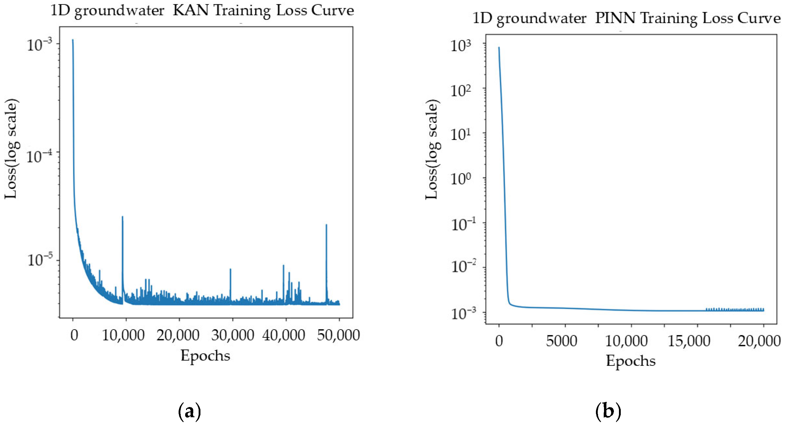
Loss curve analysis (Figure 3) further validates PKAN’s effectiveness. PKAN demonstrates rapid convergence, reducing loss values from 10⁻¹ to 10⁻⁵ in early training stages, while traditional PINN requires 2500 epochs to reach 10⁻³. Although PKAN exhibits local fluctuations around 10,000, 30,000, and 45,000 epochs, it maintains low loss levels (10⁻⁵), reflecting dynamic adjustment capabilities. Traditional PINN stabilizes after 15,000 epochs but maintains higher loss levels (10⁻³), suggesting local optima entrapment. PKAN’s superior training characteristics stem from its innovative design, including pre-training mechanisms and interlayer variation mechanisms, enhanced loss function design, and dynamic balancing strategies.

3.2. Two-Dimensional Groundwater Simulation

Two-dimensional spatial simulation better reveals complex groundwater flow characteristics. This study designed a three-well extraction scenario to compare PAKN, PINN, and finite element methods (Figure 4). The finite element results demonstrate that pumping activities created distinct drawdown cones, with hydraulic head dropping to 48.74 m near the wells while maintaining higher levels (approximately 50.54 m) in regions distant from well points. This distribution pattern accurately reflects the typical characteristics of multi-well pumping systems.

The traditional PINN method exhibits notable limitations in handling such complex spatial distributions. Although it broadly captures the spatial variation trends of hydraulic heads, significant numerical distortions emerge in local areas near extraction points, with maximum errors reaching 1.215. These simulation deviations reflect PINN’s inherent deficiencies in handling multi-source problems with sharp gradient variations.

In contrast, the PKAN framework demonstrates superior performance in 2D simulation, particularly in heterogeneous fields. First, PKAN accurately reproduces the hydraulic head extrema (48.74–50.54 m) at source-sink locations, showing excellent agreement with reference solutions. Second, in transition zones between source-sink points, PKAN precisely captures the continuous, gradual variation characteristics of hydraulic heads, demonstrating exceptional spatial resolution capability. Most significantly, the error distribution map shows a maximum error of only 0.324, nearly four times lower than traditional PINN, with errors primarily concentrated within extremely small ranges around extraction points.

Similarly, we analyzed the loss curves (Figure 5) of both approaches in a 2D simulation. PKAN’s training characteristics (left figure) exhibit richer dynamic properties. The initial loss value rapidly decreases from 10⁻¹ to 10⁻⁴, indicating quick model comprehension of primary hydraulic head distribution features. Notably, multiple sharp fluctuations appear throughout training, reflecting the model’s dynamic response to various physical constraints: larger fluctuations likely correspond to weight adjustments in high-gradient regions near well points, while smaller ones may arise from fine-tuning hydraulic responses in well interference zones.

In contrast, traditional PINN’s loss curve (right figure) shows a relatively monotonic convergence process. Though it achieves a rapid descent from 10³ to 10⁻¹ in the first 2000 epochs, the curve subsequently plateaus, maintaining at the 10⁻¹ level. This convergence characteristic reflects traditional PINN’s limitations in handling multi-center strong gradient problems: once reaching certain optimization levels, the model struggles to further improve accuracy, especially in complex scenarios requiring simultaneous satisfaction of control equations and multiple pumping boundary conditions.

From an optimization dynamics perspective, PKAN’s loss curve characteristics reveal two key advantages in 2D problems: first, lower final loss values (10⁻⁴ level) indicate a more precise description of complex hydraulic fields; second, sustained optimization capability demonstrates stronger adaptability in handling multi-scale features and balancing various physical constraints. Statistical analysis shows PINN network achieved an R² value of −0.3043 and RMSE of 0.3067, while PKAN achieved an R² value of 0.917 and RMSE of 0.077.

3.3. Sensitivity Analysis of PKAN Framework

This study conducted a sensitivity analysis of the PKAN framework (

Table 2. Sensitivity analysis results of the PKAN framework.

Sample Size	Neurons Layer	R2	RMSE	Training Time (s)
10 × 10	64	−35.639	1.6258	1517.31617
20 × 20	64	0.2746	0.228	2138.73427
50 × 50	64	0.917	0.077	16,316.60415
100 × 100	64	0.9359	0.0679	40,164.68628
Method	Configuration	R2	RMSE	Training Time (s)
Random	32 neurons/layer, 2500 points	0.5665	0.1768	1516.86485
Random	32 neurons/layer, 10,000 points	0.8991	0.0852	1499.43390
Random	64 neurons/layer, 2500 points	0.6654	0.1553	1602.19821
Random	64 neurons/layer, 10,000 points	0.7485	0.1346	2334.11892
Uniform	64 neurons/layer, 2500 points	0.9015	0.0842	16,316.60415
Neurons Layer	Configuration	R2	RMSE	Training Time (s)
32	Uniform 20 × 20	−0.1663	0.2900	1542.64965
64	Uniform 20 × 20	0.2746	0.2280	2138.73427
128	Uniform 20 × 20	0.7471	0.1350	5045.00634
32	Uniform 50 × 50	0.8907	0.0887	8171.88816

) for groundwater simulation, focusing on sampling strategies [32] and network architecture. The analysis maintained consistent three-well pumping conditions to ensure result comparability.

For sampling strategies, we examined spatial sampling density (random sampling of 2500 and 10,000 points; uniform grid sampling from 10 × 10 to 100 × 100) with fixed temporal sampling. Results show that uniform grid sampling at 50 × 50 significantly improved model performance (R² = 0.917, RMSE = 0.077). While increasing to 100 × 100 marginally improved R² to 0.9359, it substantially increased computational time from 16,316 to 40,164 s. Uniform sampling demonstrated superior performance compared to random sampling, with R² = 0.9015 for uniform sampling (50 × 50) versus R² = 0.7485 for random sampling (10,000 points) using 64 neurons.

Network architecture analysis revealed that with 20 × 20 sampling, increasing neurons per layer from 32 to 128 improved R² from −0.1663 to 0.7471. However, with 50 × 50 sampling, 32 neurons achieved satisfactory performance (R² = 0.8907). Based on computational efficiency and prediction accuracy trade-offs, we recommend a standard configuration of 50 × 50 uniform sampling points with 64 neurons per layer for the PKAN framework. This configuration provides reliable groundwater system numerical simulation results at reasonable computational cost.

4. Discussion

Our research demonstrates that PKAN represents a significant advancement in groundwater flow simulation, particularly when dealing with heterogeneous media and complex well configurations. The exceptional performance of PKAN in both 1D and 2D scenarios emerges from its innovative integration of Kolmogorov–Arnold network principles with physics-informed constraints. This architectural design effectively addresses the fundamental challenge of balancing mathematical expressiveness with physical consistency, particularly evident in handling local steep gradients near extraction wells where heterogeneity effects are most pronounced.

The sensitivity analysis of our model reveals important insights into scale-dependent heterogeneity effects in groundwater systems. We observed that as the scale increases, the influence of heterogeneity on flow patterns becomes more significant, requiring higher model resolution to accurately capture these effects. This is especially evident in multi-well pumping scenarios, where the interference patterns between wells create complex flow structures highly sensitive to the underlying heterogeneity. Our findings confirm that the variance of hydraulic conductivity (expressed as variance of lnK) significantly impacts simulation accuracy, with higher variances requiring more sophisticated modeling approaches.

The distinct training characteristics of PKAN, notably its rapid convergence to 10⁻⁵ loss levels and sustained optimization capability, reveal important insights into the learning dynamics of physics-informed neural networks in heterogeneous environments. The observed fluctuations in the loss curve demonstrate the model’s active adaptation to different physical constraints across various spatial scales, suggesting a more effective balance between exploration and exploitation compared to PINN’s tendency to settle in local optima.

While PKAN demonstrates superior accuracy in capturing heterogeneity effects, its computational requirements warrant careful consideration. The sensitivity analysis reveals a critical trade-off between sampling density and computational cost-increasing from 50 × 50 to 100 × 100 sampling points yields only a marginal improvement in accuracy but dramatically increases computational time. This relationship has significant implications for implementing PKAN in scenarios with strongly heterogeneous aquifers or multi-scale problems. The optimal configuration of 50 × 50 uniform sampling with four hidden layers and 64 neurons per layer provides sufficient resolution to capture relevant heterogeneity effects while maintaining computational efficiency.

Several challenges remain to be addressed in future research. The substantial computational resources required for training, particularly when modeling highly heterogeneous systems, necessitate the development of more efficient training strategies. Further validation is needed for multi-field coupling problems across different scales, non-standard boundary conditions, transient flow with variable boundary conditions in heterogeneous media, and three-dimensional applications with complex spatial heterogeneity patterns. The current computational requirements limit PKAN’s applicability in the real-time modeling of highly heterogeneous systems, suggesting the need for research into model acceleration techniques or hybrid approaches that can adapt to varying degrees of heterogeneity.

5. Conclusions

This study proposed a physics-informed Kolmogorov–Arnold network (PKAN) framework for solving complex groundwater flow problems. Through systematic testing and analysis of one- and two-dimensional cases, the following main conclusions were drawn:

(1) The PKAN framework demonstrates significant advantages in handling complex groundwater flow problems. In one-dimensional heterogeneous transient simulations, PKAN’s prediction accuracy (R² = 0.9966, RMSE = 0.0313) substantially outperforms traditional PINN (R² = −0.7194, RMSE = 0.7001). In two-dimensional multi-well pumping system simulations, PKAN also exhibits excellent performance (R² = 0.917, RMSE = 0.077), while traditional PINN performs relatively poorly (R² = −0.3043, RMSE = 0.3067).

(2) PKAN significantly improves model training efficiency and stability through innovative network architecture design. Loss curve analysis indicates that PKAN can quickly converge to a loss level of 10⁻⁵ in the early training stages while maintaining continuous optimization capability during long-term training. This excellent training characteristic benefits from the introduction of pre-training mechanisms and inter-layer variation mechanisms, enabling a better balance between physical constraints and numerical stability. PKAN shows unique advantages in handling local steep gradient problems. Particularly in two-dimensional multi-well pumping systems, PKAN not only accurately captures drawdown cone morphological characteristics but also precisely reproduces interference effects between multiple wells, with maximum errors only one-quarter that of traditional PINN. This demonstrates PKAN’s excellence in handling complex boundary conditions and multi-scale features.

(3) Sensitivity analysis results indicate that sampling strategy and network structure significantly influence PKAN’s performance. A configuration of 50 × 50 uniform sampling points with four hidden layers and 64 neurons per layer achieves optimal balance between computational efficiency and simulation accuracy.

However, the PKAN framework still has aspects requiring further improvement. While PKAN achieves high simulation accuracy, its training process currently requires substantial time and computational resources, somewhat limiting its potential applications in large-scale real-time simulations. We recognize the need to extend our work to 3D simulations and validate it under real field conditions. Additionally, model performance shows sensitivity to network structure and hyperparameter selection, potentially requiring detailed parameter tuning for different application scenarios. Furthermore, the current PKAN framework primarily focuses on solving flow equations, and its capabilities in handling multi-field coupling problems common in practical engineering (such as temperature fields and solute transport), as well as complex situations like irregular boundaries and discontinuous media, require further verification.

References

- Trefry, M.G.; Muffels, C. FEFLOW: A finite-element ground water flow and transport modeling tool. Groundwater 2007, 45, 525–528. [Google Scholar]
- Xie, H.-Y.; Jiang, X.-W.; Tan, S.-C.; Wan, L.; Wang, X.-S.; Liang, S.-H.; Zeng, Y. Interaction of soil water and groundwater during the freezing–thawing cycle: Field observations and numerical modeling. Hydrol. Earth Syst. Sci. 2021, 25, 4243–4257. [Google Scholar]
- Zhang, J.; Hou, R.-Z.; Yu, K.; Dong, J.-Q.; Yin, L.-H. Research Paper Impact of water table on hierarchically nested groundwater flow system. J. Groundw. Sci. Eng. 2024, 12, 131. [Google Scholar]
- Sun, J.; Hu, L.; Li, D.; Sun, K.; Yang, Z. Data-driven models for accurate groundwater level prediction and their practical significance in groundwater management. J. Hydrol. 2022, 608, 127630. [Google Scholar]
- Vilhelmsen, T.N.; Christensen, S.; Mehl, S.W. Evaluation of MODFLOW-LGR in connection with a synthetic regional-scale model. Groundwater 2012, 50, 118–132. [Google Scholar]
- Walter, D.A.; Masterson, J.P.; Finkelstein, J.S.; Monti, J., Jr.; Misut, P.E.; Fienen, M.N. Simulation of Groundwater Flow in the Regional Aquifer System on Long Island, New York, for Pumping and Recharge Conditions in 2005–15; US Geological Survey: Reston, VA, USA, 2020; ISBN 2328-0328. [Google Scholar]
- Raissi, M.; Perdikaris, P.; Karniadakis, G.E. Physics-informed neural networks: A deep learning framework for solving forward and inverse problems involving nonlinear partial differential equations. J. Comput. Phys. 2019, 378, 686–707. [Google Scholar]
- Sun, J.; Liu, Y.; Wang, Y.; Yao, Z.; Zheng, X. BINN: A deep learning approach for computational mechanics problems based on boundary integral equations. Comput. Methods Appl. Mech. Eng. 2023, 410, 116012. [Google Scholar]
- Li, Z.; Kovachki, N.; Azizzadenesheli, K.; Liu, B.; Bhattacharya, K.; Stuart, A.; Anandkumar, A. Fourier neural operator for parametric partial differential equations. arXiv 2020, arXiv:2010.08895. [Google Scholar]
- Karniadakis, G.E.; Kevrekidis, I.G.; Lu, L.; Perdikaris, P.; Wang, S.; Yang, L. Physics-informed machine learning. Nat. Rev. Phys. 2021, 3, 422–440. [Google Scholar]
- Sirignano, J.; Spiliopoulos, K. DGM: A deep learning algorithm for solving partial differential equations. J. Comput. Phys. 2018, 375, 1339–1364. [Google Scholar]
- Mahmoudabadbozchelou, M.; Karniadakis, G.E.; Jamali, S. nn-PINNs: Non-Newtonian physics-informed neural networks for complex fluid modeling. Soft Matter 2022, 18, 172–185. [Google Scholar]
- Liu, A.; Li, J.; Bi, J.; Chen, Z.; Wang, Y.; Lu, C.; Jin, Y.; Lin, B. A novel reservoir simulation model based on physics informed neural networks. Phys. Fluids 2024, 36, 116617. [Google Scholar]
- Wang, Y.; Alkhadhr, S.; Almekkawy, M. Pinn simulation of the temperature rise due to ultrasound wave propagation. In Proceedings of the 2021 IEEE International Ultrasonics Symposium (IUS), Xi’an, China, 11–16 September 2021; pp. 1–4. [Google Scholar]
- Shen, C. A transdisciplinary review of deep learning research and its relevance for water resources scientists. Water Resour. Res. 2018, 54, 8558–8593. [Google Scholar]
- Xu, R.; Wang, N.; Zhang, D. Solution of diffusivity equations with local sources/sinks and surrogate modeling using weak form theory-guided neural network. Adv. Water Resour. 2021, 153, 103941. [Google Scholar]
- Brunetti, G.F.A.; De Bartolo, S.; Fallico, C.; Rivera Velásquez, M.F.; Severino, G. Experimental investigation to characterize simple versus multi scaling analysis of hydraulic conductivity at a mesoscale. Stoch. Environ. Res. Risk Assess. 2022, 36, 1131–1142. [Google Scholar]
- Severino, G.; Fallico, C.; Brunetti, G.F.A. Correlation Structure of Steady Well-Type Flows Through Heterogeneous Porous Media: Results and Application. Water Resour. Res. 2024, 60, e2023WR036279. [Google Scholar]
- Hildebrand, F.B. Introduction to Numerical Analysis; Courier Corporation: Chelmsford, MA, USA, 1987. [Google Scholar]
- Liu, Q.; Liu, Z.; Zhu, X.; Xiu, Y. Deep active learning by model interpretability. arXiv 2020, arXiv:2007.12100. [Google Scholar]
- Liu, Z.; Wang, Y.; Vaidya, S.; Ruehle, F.; Halverson, J.; Soljačić, M.; Hou, T.Y.; Tegmark, M. Kan: Kolmogorov-arnold networks. arXiv 2024, arXiv:2404.19756. [Google Scholar]
- Braun, J.; Griebel, M. On a constructive proof of Kolmogorov’s superposition theorem. Constr. Approx. 2009, 30, 653–675. [Google Scholar]
- Hecht-Nielsen, R. Kolmogorov’s mapping neural network existence theorem. In Proceedings of the International Conference on Neural Networks, San Diego, CA, USA, 21–24 June 1987; pp. 11–14. [Google Scholar]
- Kolmogorov, A.N. On the Representation of Continuous Functions of Several Variables by Superpositions of Continuous Functions of a Smaller Number of Variables; American Mathematical Society: Providence, RI, USA, 1961. [Google Scholar]
- Sidharth, S.S.; Keerthana, A.R.; Gokul, R.; Anas, K.P. Chebyshev polynomial-based kolmogorov-arnold networks: An efficient architecture for nonlinear function approximation. arXiv 2024, arXiv:2405.07200. [Google Scholar]
- Shukla, K.; Toscano, J.D.; Wang, Z.; Zou, Z.; Karniadakis, G.E. A comprehensive and FAIR comparison between MLP and KAN representations for differential equations and operator networks. arXiv 2024, arXiv:2406.02917. [Google Scholar] [CrossRef]
- Bathe, K.-J. Finite Element Procedures; Prentice Hall, Pearson Education: Saddle River, NJ, USA, 2006. [Google Scholar]
- Bai, J.; Liu, G.-R.; Gupta, A.; Alzubaidi, L.; Feng, X.-Q.; Gu, Y. Physics-informed radial basis network (PIRBN): A local approximating neural network for solving nonlinear partial differential equations. Comput. Methods Appl. Mech. Eng. 2023, 415, 116290. [Google Scholar] [CrossRef]
- He, S.; Reif, K.; Unbehauen, R. Multilayer neural networks for solving a class of partial differential equations. Neural Netw. 2000, 13, 385–396. [Google Scholar] [CrossRef]
- Lagaris, I.E.; Likas, A.; Fotiadis, D.I. Artificial neural networks for solving ordinary and partial differential equations. IEEE Trans. Neural Netw. 1998, 9, 987–1000. [Google Scholar] [CrossRef]
- Sun, L.; Gao, H.; Pan, S.; Wang, J.-X. Surrogate modeling for fluid flows based on physics-constrained deep learning without simulation data. Comput. Methods Appl. Mech. Eng. 2020, 361, 112732. [Google Scholar]
- Zhang, X.; Zhu, Y.; Wang, J.; Ju, L.; Qian, Y.; Ye, M.; Yang, J. GW-PINN: A deep learning algorithm for solving groundwater flow equations. Adv. Water Resour. 2022, 165, 104243. [Google Scholar] [CrossRef]