Article

Spatial and Temporal Shifts and Driving Mechanisms of Embodied Carbon in Water Transport Trade in BRICS Countries

1
School of International Economics and Trade, Fujian Business University, Fuzhou 350012, China
2
College of Civil Engineering, Fuzhou University, Fuzhou 350108, China
*
Author to whom correspondence should be addressed.
Water 2025, 17(7), 1070; https://doi.org/10.3390/w17071070
Submission received: 17 February 2025 / Revised: 28 March 2025 / Accepted: 1 April 2025 / Published: 3 April 2025

Abstract

:
From an ecological protection perspective, clarifying the spatial and temporal transfer characteristics of embodied carbon in water transport trade among BRICS countries and its driving mechanisms is of great significance for the precise formulation of emission reduction policies. This study integrates the multi-regional input–output model with the LMDI decomposition method to quantitatively analyze the bi-directional flow of embodied carbon in water transport trade among BRICS countries from 1995 to 2018, along with its spatio-temporal differentiation patterns. The driving mechanisms are decomposed across three dimensions: scale, structure, and intensity. By adopting a dual perspective of time-series and spatial correlation, the study systematically uncovers the cross-regional transfer patterns of embodied carbon emissions in water transport trade and examines the interaction pathways of various effects throughout their dynamic evolution. The study finds that (1) the embodied carbon in water transport trade among BRICS countries shows a trend of transnational transfer, with China being the largest net exporter (35.15 Mt in 2018), India and South Africa as net importers (−32.00 Mt and −1.89 Mt in 2018, respectively), and Brazil and Russia shifting from net importers to net exporters; (2) from a temporal perspective, the scale effect drives the growth of embodied carbon emissions (contribution values: 1.23~119.72 Mt for export trade; 4.88~34.36 Mt for import trade), while the intensity effect has a suppressive role (contribution values: −59.08~−1.48 Mt for export trade; −20.56~−5.31 Mt for import trade), and the structural effect is complex in its impact on emissions (contribution values: −17.72~0.45 Mt for export trade; −6.84~13.93 Mt for import trade). Optimizing the trade structure can help reduce carbon emissions; (3) from a spatial perspective, carbon emissions are higher in Southeast Asia and the Northern Hemisphere, and changes in China’s carbon emissions (total effect in 2018: 57.01 Mt in export trade and 7.98 Mt in import trade) significantly affect other BRICS countries. Based on the conclusions of the study, it is suggested that BRICS countries should strengthen cooperation to achieve regional emission reduction targets by optimizing the trade structure of water transport, promoting energy structure reforms, advancing green transport technologies and equipment, and establishing a carbon emission regulatory system.

1. Introduction

The global shipping industry handles approximately 90% of international trade, but its immense contribution to economic activities comes at a significant environmental cost—shipping. As a major source of greenhouse gas emissions, shipping increasingly drives climate change, and pollution costs have become progressively apparent [1]. Extensive research has been conducted on the environmental impacts of ships and related industries. For example, Premsamarn et al. [2] analyzed Automatic Identification System (AIS) data from the Gulf of Thailand to evaluate the emission reduction effects of Emission Control Area (ECA) policies on NOX, SOX, and particulate matter (PM). They identified tankers as the primary regional pollutant source and recommended measures such as low-sulfur fuels and route optimization to significantly reduce emissions, thereby providing a scientific basis for maritime emission reduction strategies in Southeast Asian countries. Similarly, Sha et al. [3] examined vessel entry and exit data from 189 global ports, systematically analyzing emission characteristics across different vessel types, seasons, and geographic regions. Their study confirmed that tankers and container ships are the main contributors to emissions, and they noted that hubs such as Singapore, Rotterdam, and Antwerp exhibit the highest emission intensities, which supports refined port-level emission management. Additionally, da Silva et al. [4] developed an AIS-based ship emission estimation framework by decoding vessel trajectories, integrating technical parameters with operational characteristics, and incorporating port-terminal vessel identification algorithms, significantly improving emission accounting accuracy. Notably, Yeh et al. [5] analyzed exhaust components from 16 different vessel types and found that naphthalene (Nap) accounts for 77–97% of polycyclic aromatic hydrocarbons (PAHs), with some vessels exceeding safety thresholds, posing direct threats to air quality and public health in port cities.
Due to its global and persistent nature, embodied carbon emissions from water transport have drawn considerable attention. Zheng et al. [6] employed input–output analysis combined with the Logarithmic Mean Divisia Index (LMDI) decomposition model to reveal that, despite ongoing efforts to achieve a low-carbon transition, the expansion of economic scale remains the dominant driver of carbon emissions in China’s water transport sector, while improvements in energy efficiency and the adoption of clean technologies have effectively mitigated this trend. In this context, carbon intensity metrics have become key tools in balancing economic growth with emission reduction targets. Jaramillo et al. [7] compared four carbon intensity indicators for port tugboats, finding that those based on energy consumption are more practical due to their low variability and strong correlation with operational characteristics, whereas average load indicators, due to high dispersion, are less applicable. This highlights the importance of aligning indicator design closely with vessel-specific attributes. To achieve deep decarbonization, Raftis et al. [8] systematically evaluated the potential of alternative fuels for inland shipping, noting that while liquefied natural gas (LNG) was initially viewed as a transitional solution, battery and hydrogen technologies are emerging as focal points in Europe and Asia. Furthermore, Billington et al. [9] provided empirical evidence that renewable diesel, when used to replace conventional low-sulfur diesel, can reduce tugboat exhaust CO2 emissions by 6%, offering a feasible pathway for short-term emission reductions.
Accurately quantifying embodied carbon in trade is fundamental for devising effective emission reduction strategies. Embodied carbon refers to the total greenhouse gas emissions generated throughout the production and supply chain of goods and services [10]. The primary methods for its calculation are as follows: (1) bottom-up Life Cycle Assessment (LCA), which is suitable for countries with comprehensive data or specific product analyses but is challenging to extend to the macro level [11]; (2) the IPCC standardized approach, which uses standard coal equivalence and sectoral emission factors to ensure cross-regional comparability for macro-scale studies [12]; and (3) input–output analysis (IOA), a top-down method that quantifies economy-wide emissions and analyzes inter-industry linkages, widely applied in energy and environmental research [13]. These methods provide a scientific basis for identifying high-carbon segments and optimizing supply chain management [14,15]. Furthermore, Al-Abdulqader et al. [16] conducted a cross-country empirical study demonstrating that carbon trading systems are more effective than carbon tax policies in driving emission reductions, emphasizing the need for tailored carbon pricing mechanisms that account for national economic structures and political contexts.
Despite significant advances, a systematic analysis of the spatiotemporal transfer and driving mechanisms of embodied carbon in water transport trade among BRICS countries (Brazil, Russia, India, China, and South Africa) [17] is still lacking. This study utilizes OECD Multi-Regional Input–Output (MRIO) tables and the LMDI decomposition method to elucidate the spatiotemporal patterns and driving factors of carbon emissions in the water transport sector among BRICS nations, thereby providing theoretical support and practical guidance for the formulation of differentiated emission reduction policies and regional low-carbon cooperation.

2. Methodology

2.1. Basic Principles of Input–Output Analysis

The input–output method visualizes the interrelations among various sectors in the national economy by constructing an input–output table. This method uses direct consumption coefficients to establish a functional relationship between production and consumption. According to traditional economic theory, total demand equals total supply; combined with the concept of intermediate products, the input–output balance is expressed as follows:
X = A X + Y
where X represents the total output column vector, Y is the final demand matrix (comprising domestic final demand Y D and export demand Y E ), and A is the direct consumption coefficient matrix, indicating the direct inputs required from various sectors to produce one unit of the final product.
Through derivation, total output can be further expressed as follows:
X = ( I A ) 1 Y = C Y
Here, ( I A ) 1 is known as the Leontief inverse or complete demand coefficient matrix C , whose elements represent the total inputs required from each sector to obtain one unit of a sector’s final product.
The use of complete demand coefficients allows for a more comprehensive reflection of resource consumption during production, which is critical for precise assessments of carbon emissions and resource consumption.

2.2. Calculation Methods for Trade-Embodied Carbon Emissions

2.2.1. Fundamental Formula for Measuring Trade-Embodied Carbon Emissions

Let e d denote the direct carbon emission per unit output (i.e., the direct carbon emission coefficient) for each industry sector, where the elements of the row vector e d = e 1 d , e 2 d , , e j d represent the direct carbon emission coefficients for the respective sectors. Let F d represent the total carbon emissions for all sectors in a country, i.e.,
F d = e d X
where X is the total output column vector. Substituting Equation (3) into Equation (2), we obtain
F d = e d X = e d ( I A ) 1 Y = E d Y
where E d represents the complete carbon emission coefficient, i.e., ( I A ) 1 , and Y is the final demand vector.
Consequently, the calculation formula for trade-embodied carbon emissions, T C , is given by
T C = e d ( I A ) 1 T V
where T V denotes the trade volume (export volume, import volume, or net export volume).

2.2.2. Classification and Calculation Formulas for Trade-Embodied Carbon Emissions

Drawing upon previous studies [18], the embodied carbon emissions involved in the production process are further subdivided according to the production and consumption countries into four categories:
Category I: embodied carbon emissions from domestic production with domestic consumption:
X = e d ( I A d ) 1 Y D = E d Y D
where e d represents the domestic direct carbon emission coefficient, ( I A d ) 1 is the domestic full-demand matrix, and Y D is the final domestic use vector.
Category II: embodied carbon emissions from domestic production but exported:
X = e d ( I A d ) 1 Y E
where Y E represents the export vector.
Category III: embodied carbon emissions from direct consumption of imports:
X = E d A m I A d 1 Y D + E i m Y m
where E d A m I A d 1 Y D represents the portion of imported products used domestically after processing, and E i m Y m represents the portion of imported products directly used for domestic consumption. E d A m I A d 1 denotes the domestic full carbon emission coefficient for imports, E i m denotes the full carbon emission coefficient of the importing country, and Y m is the final use vector for imported products.
Category IV: embodied carbon emissions from re-export of imported intermediate inputs:
X = E d A m ( I A d ) 1 Y E
Based on this, the aggregates are defined as follows:
Total embodied carbon on the production side (EEP):
E E P = X + X = e d I A d 1 ( Y D + Y E ) = e d ( I A d ) 1 Y
Total embodied carbon on the consumption side (EEC):
E E C = X + X = E d Y D + E d A m I A d 1 Y D + E i m Y m
Export embodied carbon (EEE):
E E E = X + X = E d Y E + E d A m ( I A d ) 1 Y E
Imported embodied carbon (EEI):
E E I = X + X = E d A m I A d 1 Y + E i m Y m
Net embodied carbon transfer (EETB):
E E T B = E E E E E I = E E P E E C

2.3. LMDI Decomposition Model in Temporal Dimension

Grossman and Krueger [19] examined the mechanisms by which trade liberalization impacts environmental pollution, proposing that international trade influences environmental quality through scale, structure, and intensity effects. The scale effect refers to the increase in energy consumption and carbon emissions resulting from trade expansion, while the structure effect reflects changes in trade composition impacting pollutant emissions. The intensity effect indicates that technological innovation can reduce carbon emissions, thereby improving overall environmental quality. Based on an extended Kaya–LMDI framework, this study develops a model for analyzing the driving factors behind embodied carbon emissions in water transport trade:
C w = T × T w T × C w T w
where C w is the total trade-embodied carbon emissions of the country’s water transport sector (in million tons); T is the total foreign trade of the country (in million USD); and T w is the foreign trade volume of the country’s waterway transport sector (in million USD).
The equation is further transformed, as shown below:
C w = Q × S w × R w
where Q = T represents the trade scale (i.e., total trade volume), reflecting the scale effect; S w denotes the trade structure of water transport, i.e., the proportion of water transport in overall trade, which reflects the structural characteristics of the transportation mode and embodies the structure effect; and R w represents the embodied carbon emission intensity of water transport (embodied carbon emission per unit trade volume), reflecting the intensity effect.
Using the LMDI additive decomposition model, the change in trade-embodied carbon emissions of the country’s water transport sector from year 0 to year t (total effect C w ) is determined by the scale effect C Q , structural effect C S , and intensity effect C R , with the following relationship between the effects:
The total effect is decomposed as follows:
C w = C w t C w 0 = Q t S w t R w t Q 0 S w 0 R w 0 = C Q + C S + C R
The formulas for calculating each effect are as follows:
Scale effect:
C Q = C w t C w 0 l n C w t l n C w 0 ln C Q t C Q 0
Structural effect:
C s = C w t C w 0 l n C w t l n C w 0 ln C S t C S 0
Intensity effect:
C R = C w t C w 0 l n C w t l n C w 0 ln C R t C R 0

2.4. LMDI Decomposition Model in Spatial Dimension

To quantify the spatial differences in the influencing factors of trade-embodied carbon in the water transport industry across different regions (BRICS countries), and to facilitate direct comparisons of spatial differences, the average of the water transport trade-embodied carbon of BRICS countries is used as a benchmark. A spatial LMDI decomposition model is constructed to analyze the spatial differences in the influencing factors of trade-embodied carbon in 1995, 2003, 2011, and 2018. The model is built as follows:
The change in water transport trade-embodied carbon between region i and benchmark u is expressed as follows:
C w ( i u ) = C w i C w u = C Q ( i u ) + C S ( i u ) + C R ( i u )
The formulas for calculating each effect are as follows:
Scale effect:
C Q ( i u ) = C w i C w u l n C w i l n C w u ln C Q i C Q u
Structural effect:
C S ( i u ) = C w i C w u l n C w i l n C w u ln C s i C s u
Intensity effect:
C R ( i u ) = C w i C w u l n C w i l n C w u ln C R i C R u
where C w i is the water transport trade-embodied carbon emissions of region i during the study period, and C w u is the average trade-embodied carbon emissions of the water transport industry across all regions during the study period, i.e., those of benchmark region u ; C Q u , C s u , and C R u are the benchmark values for scale effect, structural effect, and intensity effect, respectively; C Q ( i u ) , C S ( i u ) , and C R ( i u ) are the differences in the contributions of scale, structure, and intensity effects to trade-embodied carbon emissions between region i and the benchmark region u .

2.5. Data Sources and Processing

2.5.1. Data Sources

This study uses the Inter-Country Input–Output (ICIO) Tables from the Organization for Economic Co-operation and Development (OECD) as its primary database. Compared to other mainstream international input–output databases (e.g., EORA, EXIOBASE, WIOD), the OECD ICIO database offers the following advantages: (1) extensive coverage—it comprehensively covers time-series data from 1995 to 2018 for the BRICS countries (Brazil, Russia, India, China, South Africa), meeting the needs of long-term dynamic analysis for emerging economies; (2) standardized industry classification—it is constructed based on the United Nations’ International Standard Industrial Classification (ISIC Rev.4), which organizes industries into 45 sectors, ensuring data comparability across countries; (3) traceability of carbon emission data—the accompanying Trade in Embodied CO2 Database provides industry-specific direct emission factors and detailed energy consumption data, supporting precise calculation of embodied carbon emission.
Therefore, this study is based on the OECD database, selecting 1995–2018 as the primary research period, with the research subject being the water transport sector. The input–output data and import–export trade data are sourced from the OECD ICIO, and the carbon emission coefficient data are obtained from the OECD Trade in Embodied CO2 Database.

2.5.2. Industry Scope Definition

To ensure data availability and consistency in statistical definitions, this study employs the non-competitive input–output tables from the OECD ICIO, whose industry classification strictly follows ISIC Rev.4. ISIC Rev.4, developed by the United Nations Statistics Division under the Economic and Social Council. It is the internationally recognized standard for classifying economic activities, ensuring consistency and comparability of cross-country data. In the ICIO framework, the classification of economic sectors directly maps to the four-digit codes of ISIC Rev.4.
This study focuses on the embodied carbon emission in water transport trade, with data extracted from the OECD ICIO. The research subject is the D50 water transport sector, which corresponds to ISIC Rev.4′s Class 501 (sea and coastal water transport) and Class 502 (inland water transport). This classification covers all water transport activities for both goods and passengers (see Table 1). Through the mapping between ISIC Rev.4 and the ICIO, this study ensures data consistency with international standards and provides a clear industry scope for the analysis.

3. Results and Discussion

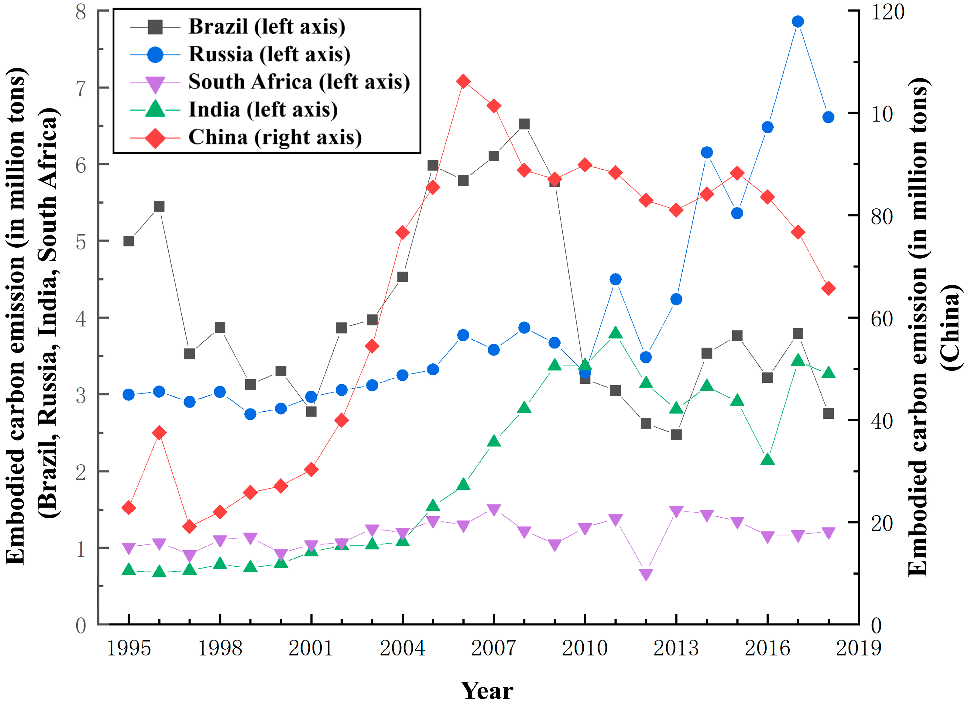
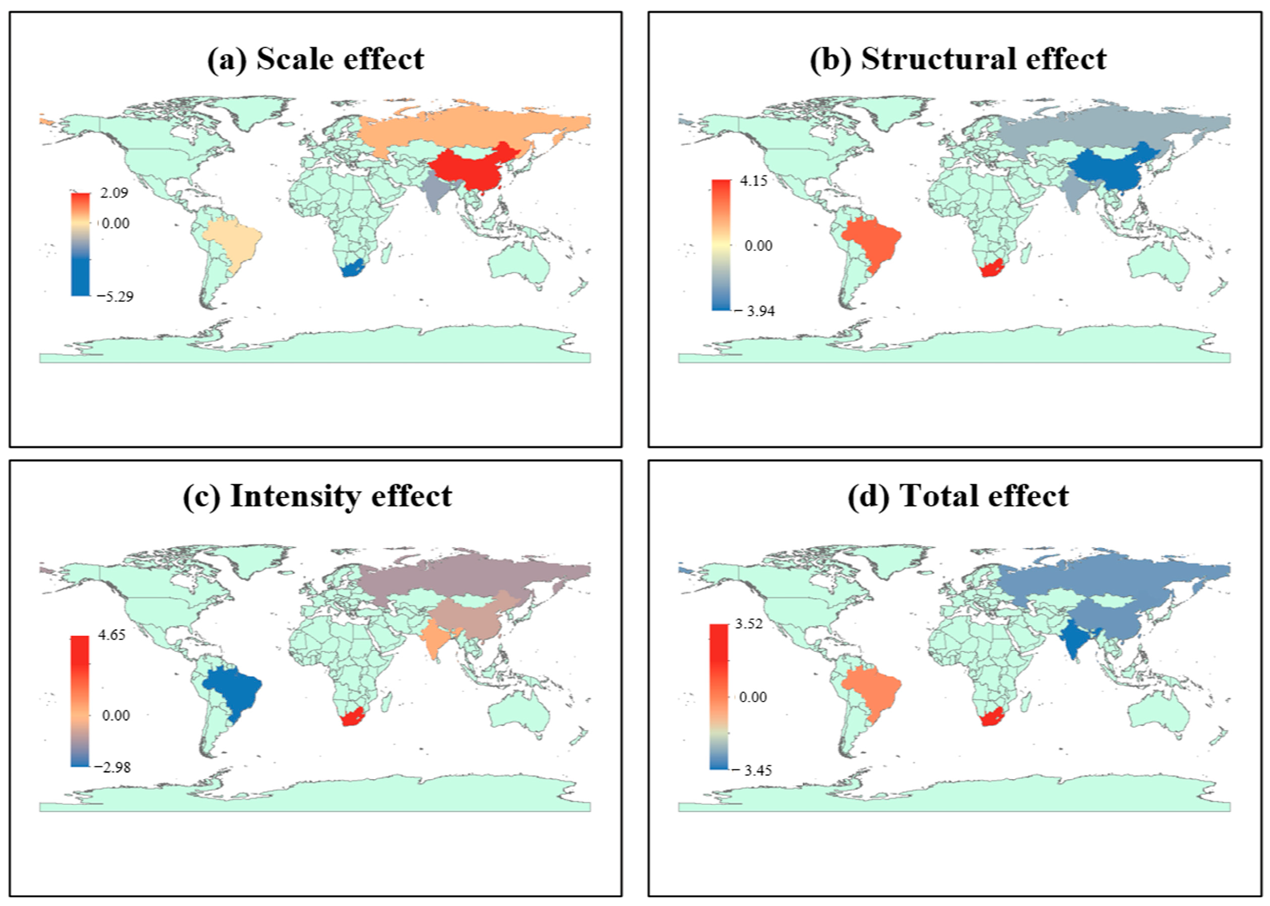
3.1. Evolution of the Pattern of Net Trade-Embodied Carbon Flows

The embodied carbon in export trade was calculated and is shown in Figure 1. China’s waterway transport industry continues to lead in total embodied carbon for export trade, increasing from 22.81 Mt in 1995 to 65.74 Mt in 2018, with an average annual growth rate of 4.71 percent. Notably, its growth rate shows phased fluctuations: it grew at an average annual rate of 6.24 percent from 2003 to 2011 due to trade expansion, and then slowed down to −9.35 percent from 2015 to 2018 due to the impact of emission reduction policies. Among the other four countries, Brazil’s embodied carbon in export trade in the waterway transport industry showed a “U-shaped” fluctuation: it dropped by 44.3 percent from 1995 to 2001, and then rebounded to 6.11 Mt (an increase of 120 percent) from 2001 to 2007. India’s embodied carbon in export trade in the waterway transport industry has been growing steadily, from 0.7 Mt in 1995 to 3.27 Mt in 2018, with the growth rate of the waterway transport industry in the past two years continuing to rise. South Africa’s total embodied carbon in export trade in the waterway transport sector was the lowest, fluctuating gently, increasing from 1.01 Mt in 1995 to 1.21 Mt in 2018. Notably, during the global financial crisis (2007–2010), embodied carbon in export trade in China’s waterway transport sector declined by 11.39 percent, while Russia led the trend of growth, and India maintained positive growth, reflecting the resilience of its trade.
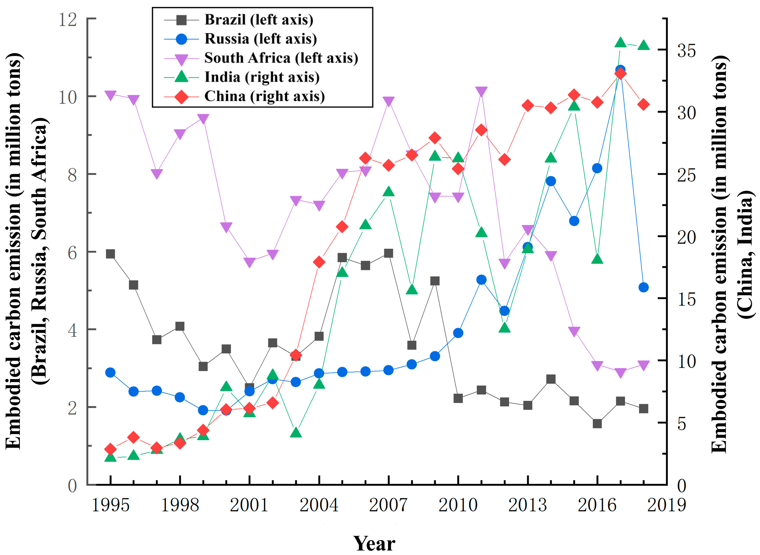
The embodied carbon in import trade was calculated and is shown in Figure 2. India’s embodied carbon emissions in water transport import trade have experienced the highest growth rate, surging from 2.15 Mt in 1995 to 35.27 Mt in 2018, with an average annual growth rate of 12.93%. Notably, this growth accelerated after 2010, with an average annual increase of 3.77% from 2010 to 2018. China ranks second in terms of growth rate, with the highest total embodied carbon emissions in water transport import trade, reaching 30.59 Mt in 2018. However, its growth rate is slower than India’s, with an average annual increase of 10.85%. In contrast, Brazil, Russia, and South Africa showed a downward trend. Brazil’s embodied carbon emissions in water transport import trade decreased from 5.94 Mt in 1995 to 1.96 Mt in 2018, reflecting an average annual decline of 4.68%. Russia’s emissions rose from 2.89 Mt to 5.08 Mt, though this was influenced by a peak of 10.67 Mt in 2017. South Africa saw its emissions drop from 10.05 Mt to 3.10 Mt, with an average annual decrease of 4.98%, indicating a significant reduction.
Looking at the data in phases, the global financial crisis of 2008 triggered a pullback in import carbon emissions across several countries. For instance, China’s import carbon emissions fell from 26.51 Mt in 2008 to 25.43 Mt in 2010, while Brazil’s emissions dropped from 3.59 Mt to 2.22 Mt in the same period. In contrast, India’s emissions increased from 15.61 Mt to 26.24 Mt, reflecting a rebound of 68%. After 2015, South Africa experienced a sharp decline in import carbon emissions, from 9.90 Mt to 3.10 Mt, aligning with its low-carbon port renovation policies.
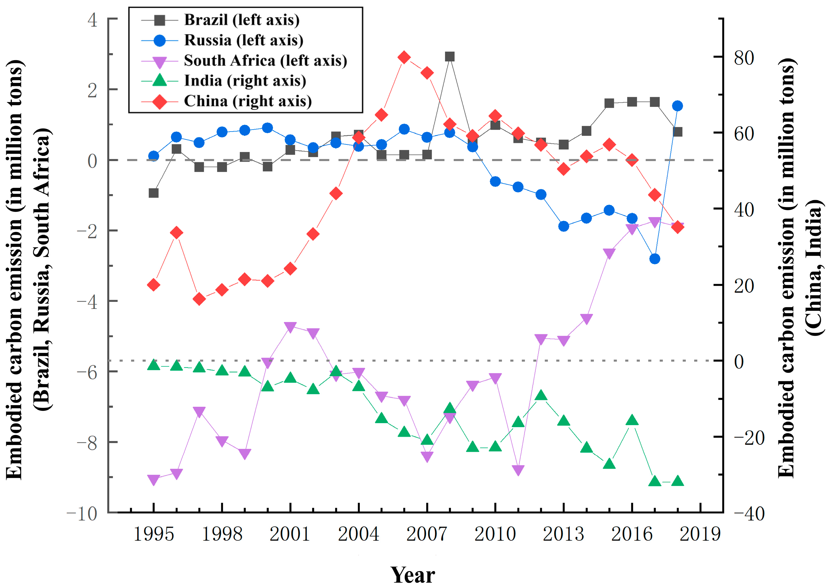
The embodied carbon in net export trade was calculated and is shown in Figure 3. China has consistently been a net exporter, with its net transfer increasing from 19.95 Mt in 1995 to a peak of 79.91 Mt in 2006, before declining to 35.15 Mt in 2018, a decrease of 56.01%. This decline supports the assertion that “emission reduction policies have begun to show results.” India’s net import gap has continued to expand, from −1.45 Mt in 1995 to −32.00 Mt in 2018, with an average annual growth rate of 11.3%. Since 2000, Brazil has shifted from a net importer (−0.19 Mt) to a net exporter (0.79 Mt in 2018), though with significant fluctuations, peaking at 2.93 Mt in 2008. Russia, after a role reversal in 2009, remained a net importer from 2010 to 2017, but in 2018 became a net exporter of 1.53 Mt, reflecting its shift in energy export structure. South Africa’s net import gap has gradually narrowed from −9.04 Mt in 1995 to −1.89 Mt in 2018, due to reductions in its import scale and improvements in energy efficiency.

3.2. Decomposition of Driving Effects in Temporal Dimension

Leveraging the temporal LMDI model, this study decomposes the driving factors of embodied carbon emissions within the export and import trade of the water transport industry across BRICS nations from 1995 to 2018, with a particular focus on the temporal heterogeneity characteristics of scale, structure, and intensity effects. The findings reveal significant national disparities and stage-wise fluctuations in both export and import trade effects (Table 2: Export trade, Table 3: Import trade).
The scale effect is the core driver of carbon emission growth, but the paths differ significantly across countries. Specifically, in terms of exports, China’s export scale effect contribution is the highest, reaching 119.72 Mt from 1995 to 2018, with a total contribution rate of 278.91%. Notably, from 2003 to 2011, the contribution rate surged to 296.87%, primarily due to the sharp increase in port throughput driving bulk commodity exports. India’s export scale effect contribution is relatively low, at just 4.33 Mt, but from 2011 to 2018, its contribution rate turned negative, dropping by −144.86%, reflecting stagnation in water transport exports, likely due to bottlenecks in port infrastructure. South Africa’s scale effect showed significant volatility, with a contribution rate of 929.12% from 2003 to 2011, mainly driven by a short-term surge in coal exports. However, from 2011 onwards, the contribution turned negative, possibly due to fluctuations in international energy prices leading to a contraction in exports. Russia’s export scale effect remained overall positive, contributing 7.95 Mt, but from 2011 to 2018, it turned negative (−0.68 Mt). Brazil’s export scale effect was relatively stable, with a contribution of 5.98 Mt, experiencing a slight decline only from 2011 to 2018.
In terms of imports, scale expansion is particularly evident in developing countries. India’s import scale effect contributed the most, with 32.06 Mt from 1995 to 2018, accounting for 96.79% of its total embodied carbon emissions. However, after 2010, the growth rate slowed to 28.46%, reflecting the gradual substitution of imports by domestic manufacturing. China’s import scale effect exhibited a phased characteristic: from 2003 to 2011, the contribution rate was 141.52%, corresponding to the deep integration of global supply chains; after 2011, it surged to 528.28%, indicating the carbon leakage risks associated with domestic consumption upgrades.
Structural effects exhibit regional heterogeneity. China’s structural effect contribution remains positive, indicating its impact on embodied carbon emissions is above the average, promoting carbon emissions. Brazil’s contribution value sharply dropped to −0.18 Mt in 2011, but it remained positive in other years with a decreasing trend, suggesting that while its impact was above the average, it was gradually converging towards the mean. The structural effect contributions of the other three countries were all negative, indicating their structural effects were below the average, thus inhibiting export-related embodied carbon emissions. Overall, before 2011, the structural effect differences between countries expanded, but in recent years, due to industrial adjustments and optimization, these contributions have decreased, narrowing the spatial distribution gap between countries.
The import structural optimization effect is significantly influenced by policy tools. South Africa’s import structural effect contribution rate was 91.01% (contribution value of −6.42 Mt) from 2011 to 2018, closely linked to its implementation of a green tariff policy. Brazil’s import structural effect was unusually negative from 2003 to 2011 (−93.62%), primarily due to the substitution of iron ore imports with local mining. India’s import structural effect contributed 54.79% (contribution value of 8.25 Mt) from 2011 to 2018, reflecting its expanding industry’s increasing dependence on high-carbon intermediate goods.
Intensity effects generally play a role in emission reduction. In terms of exports, intensity effects reflect the differences in technological advancements, with China showing the most notable improvement. From 1995 to 2018, China’s intensity effect contributed −59.08 Mt, with a contribution rate of −137.62%. Particularly from 2003 to 2011, the contribution rate reached −232.55%, confirming that China’s energy efficiency revolution in the water transport sector had begun to show results. India’s intensity effect was overall negative, with a cumulative contribution rate of −76.19%, but from 2011 to 2018, it turned positive, with a contribution rate of 87.23%, indicating that the technological upgrades in India’s water transport industry lagged behind its economic growth. Russia’s intensity effect exhibited fluctuations, being positive from 2011 to 2018, with a contribution rate of 54.09%, and negative in other years.
For imports, the intensity effect reveals the asymmetry of technological spillovers. China’s import intensity effect from 2011 to 2018 had a contribution rate of −483.46%, the highest among the five countries. This could be attributed to the adoption of ultra-large container ships (ULCVs), which reduced carbon emissions per unit of freight, reflecting China’s strong ability to absorb low-carbon technologies. South Africa, in contrast, had a contribution rate of −4.51% during the same period, reflecting limited improvements in technology. Brazil’s import intensity effect was unusually positive in 2003–2011 (685.32%), which may be linked to the rebound effect due to the failure of biofuel technology promotion.
In terms of total effects, from 1995 to 2018, China’s export total effect was 42.93 Mt, ranking the highest among the five countries, with the scale effect contributing 278.91%. India had the fastest growth, with a total effect of 2.56 Mt, and the structural effect contributed 41.45%. Russia’s total effect increased from 0.12 Mt from 1995 to 2003 to 2.11 Mt from 2011 to 2018, driven by energy strategy adjustments.
For import total effects, from 1995 to 2018, India had the largest total effect, contributing 33.12 Mt, predominantly driven by the scale effect (96.79%). China’s import total effect was 27.73 Mt, far exceeding other countries, with technological improvements (intensity effect) offsetting some of the growth (−74.15%). South Africa’s import total effect worsened from −2.72 Mt (1995–2003) to −6.95 Mt (2011–2018), primarily driven by structural effects (contribution rate of 98.36%).

3.3. Characteristics of the Distribution in Spatial Dimensions

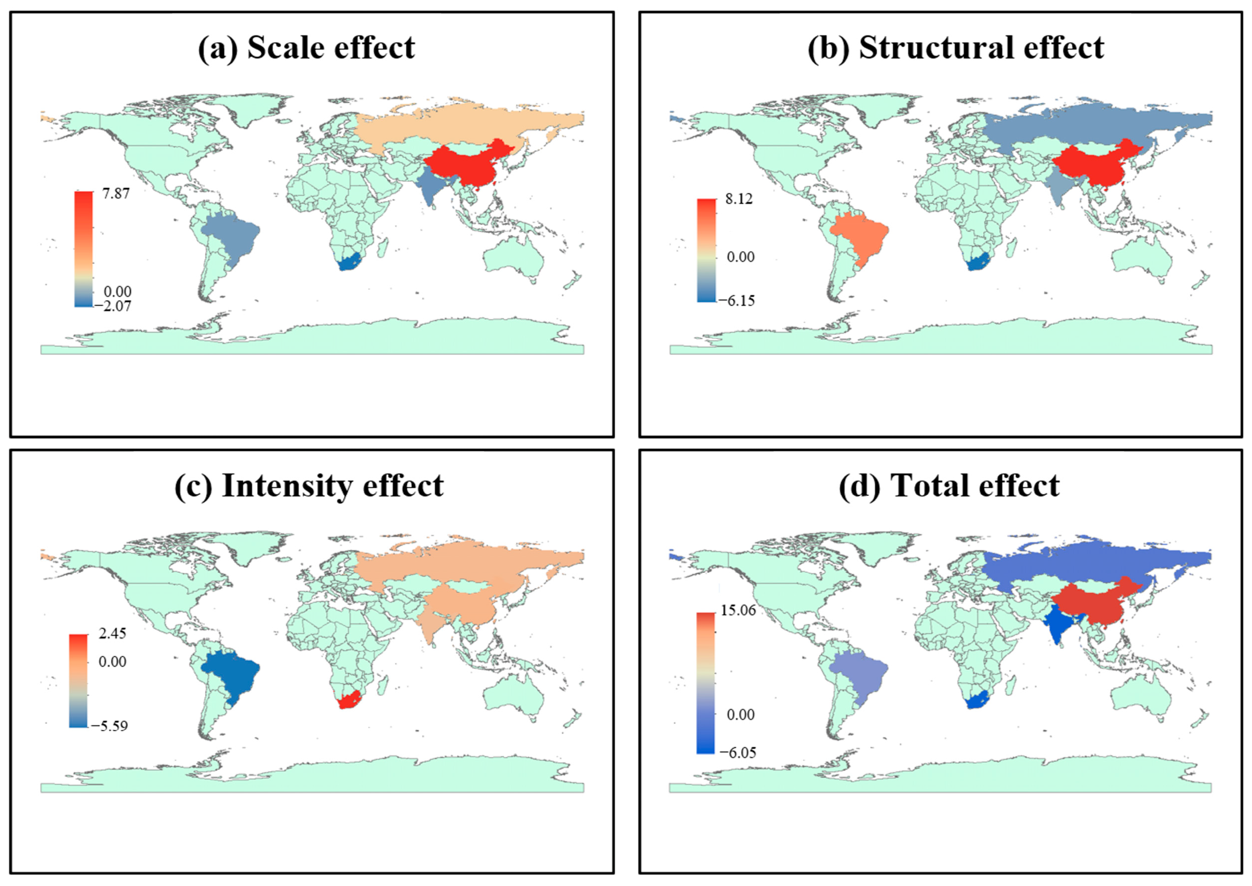
This study employs the spatial LMDI model, using the average embodied carbon emissions in the import/export trade of the water transport industry in the BRICS countries from 1995 to 2018 as a benchmark. The model reveals the spatial heterogeneity characteristics of the scale, structure, intensity, and total effects. By comparing the differences between each influencing factor and the average level, the model facilitates direct comparisons between regions. A positive decomposition result indicates that the factor’s impact on carbon emissions is above the average, contributing to an increase in emissions. Conversely, a negative result suggests that the factor’s impact is below the average, leading to a suppression of carbon emissions.

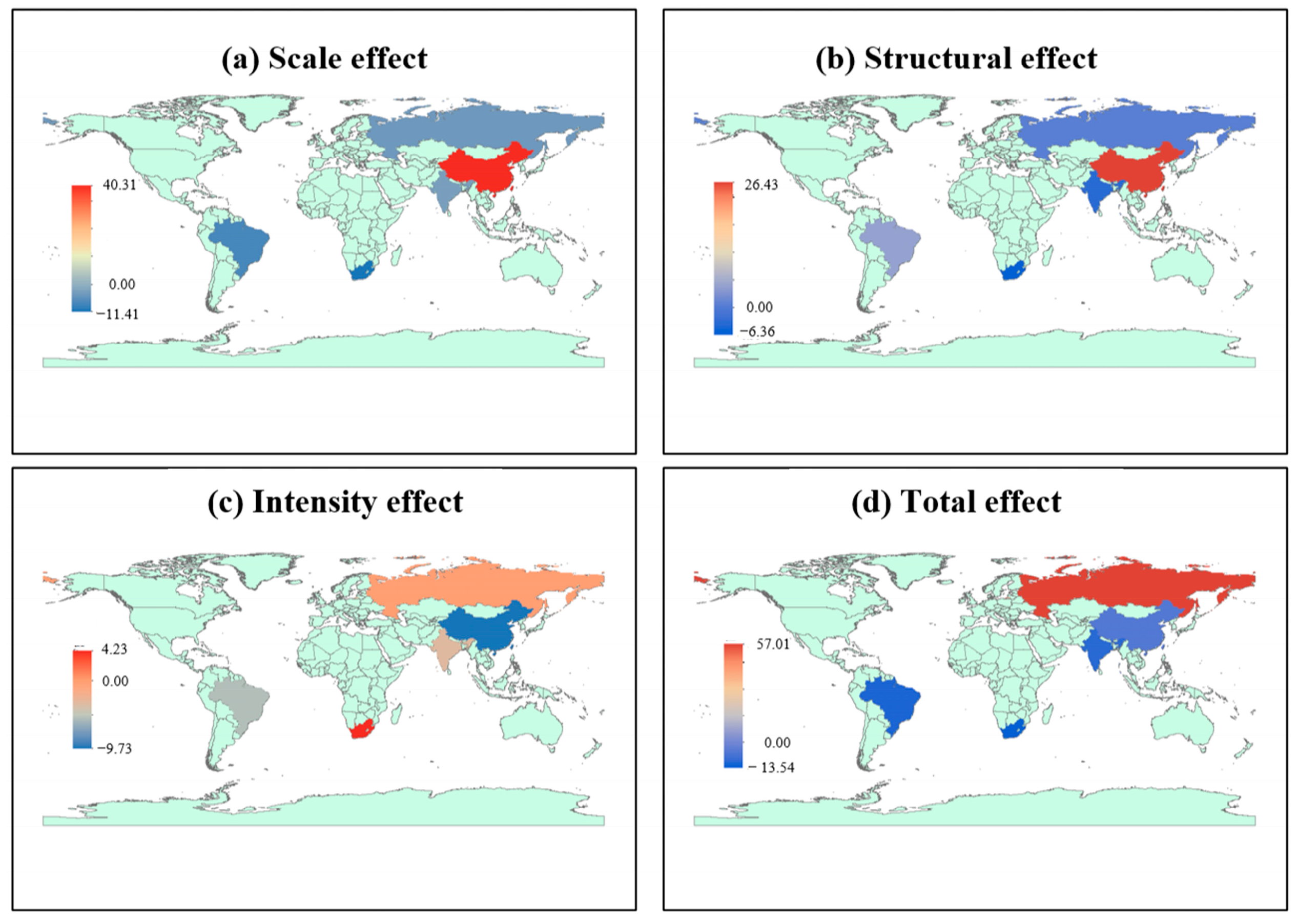
3.3.1. Spatial Dimension Analysis of Embodied Carbon in Export Trade

The spatial differentiation characteristics of export-related embodied carbon in the water transport trade of BRICS countries exhibit distinct country-specific differences (see Figure 4 and Figure 5).
In terms of scale effects, the export scale effects of the BRICS countries significantly influence the spatial differences in embodied carbon emissions. China’s export scale effect contribution is the highest, increasing from 7.87 Mt in 1995 to 40.31 Mt in 2018, and peaking at 46.92 Mt in 2011, far exceeding the average level of the five countries. This indicates that the expansion of China’s trade volume plays a dominant role in the growth of embodied carbon emissions. The contributions of the other four countries are negative, indicating that their export scale effects are below the average level and have a suppressive effect on carbon emissions. Since 2003, due to international trade friction, China’s export growth has slowed, while the total trade volume of the other four countries has increased, reducing the spatial differences in scale effects.
Structural effects show obvious regional heterogeneity. China’s structural effect contribution remains positive, indicating that its structural effect has a greater impact than the average level, promoting carbon emissions. Brazil’s contribution sharply dropped to −0.18 Mt in 2011, but remained positive in other years, showing a decreasing trend. This suggests that Brazil’s structural effect, though above the average level, is gradually converging to the mean. The contributions of the other three countries are all negative, indicating that their structural effects are below the average, thus suppressing carbon emissions. Overall, before 2011, the structural effect differences between the countries expanded. However, in recent years, due to industrial adjustments and optimization, the contribution rates have declined, narrowing the spatial distribution gap between the countries.
The intensity effects reflect technological differences. South Africa’s spatial intensity effect contribution has always been positive, with a contribution of 4.23 Mt in 2018, indicating that its energy efficiency level is above the average of the five countries. The intensity effect contributions of Brazil, Russia, and India are all negative, suggesting that their energy efficiency improvements and environmental policies are less effective than the regional average. Before 2003, China’s intensity effect was below the average, but its contribution value of 1.93 Mt in 2003 exceeded the average level, reflecting that during this period, China’s water transport trade expanded at the cost of the environment. After 2011, China’s intensity effect turned negative, indicating that technological progress in China’s water transport industry effectively suppressed spatial embodied carbon emissions.
In terms of total effects, from 1995 to 2018, China’s export total effect was always positive and far exceeded the average of the five countries, with a contribution of 42.93 Mt. Russia and India had contribution values close to the mean, indicating the “high in the East, low in the West” spatial distribution of embodied carbon emissions in BRICS exports. From the perspective of changes, the export embodied carbon is gradually shifting towards Southeast Asia, and countries are narrowing the spatial distribution gap with average levels.

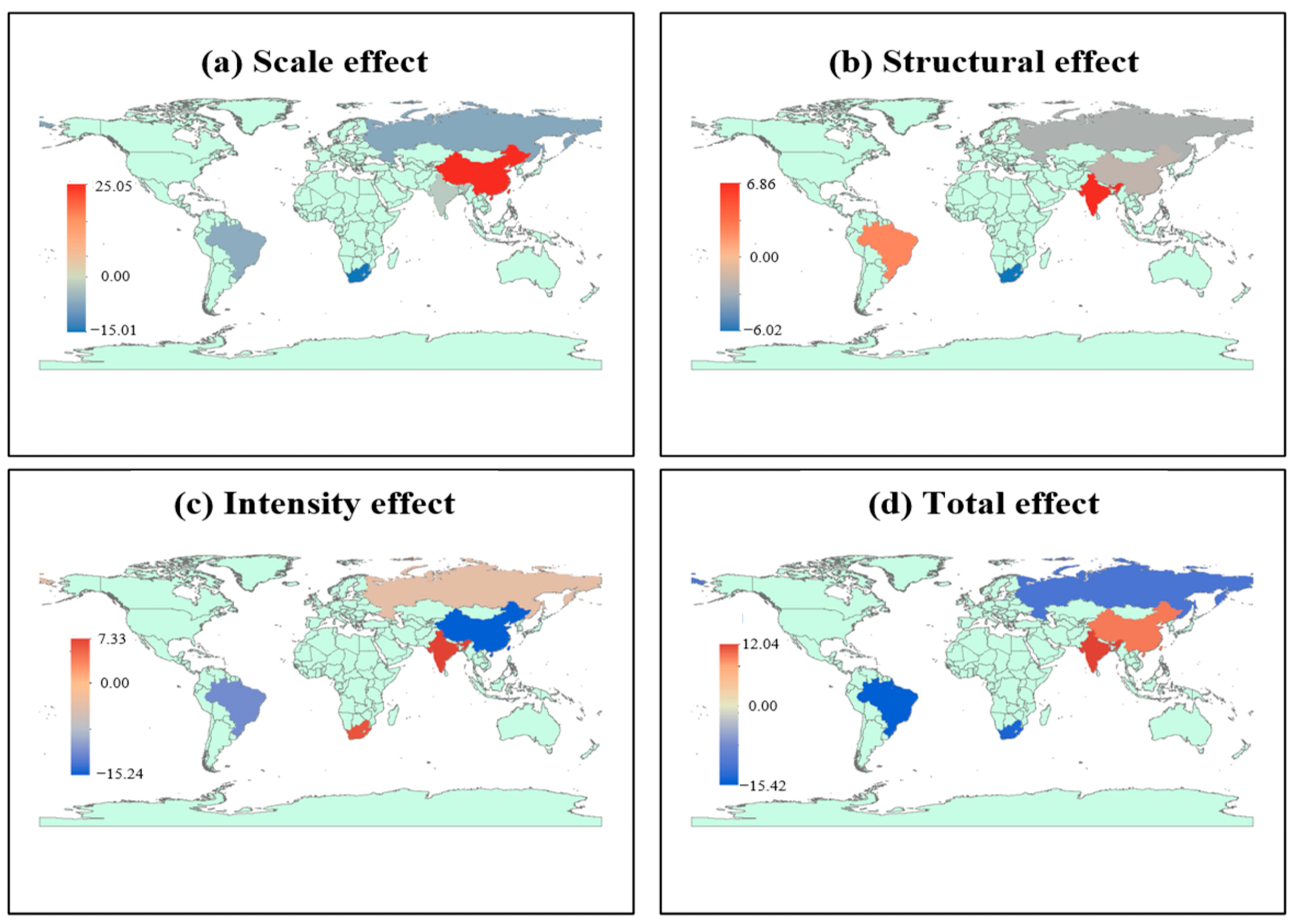
3.3.2. The Spatial Dimension Analysis of Embodied Carbon in Import Trade

The spatial differentiation characteristics of embodied carbon in the import trade of the BRICS countries exhibit significant asymmetry compared to export trade, with the driving mechanisms of the scale, structure, and intensity effects showing distinct country-specific heterogeneity (see Figure 6 and Figure 7).
In terms of import scale effects, the spatial distribution of the countries is similar to that of export trade. China’s import scale effect contribution steadily increased from 2.09 Mt in 1995 to 25.05 Mt in 2018; although its growth rate was slower than exports, it still shows significant growth. The import scale effect contributions of the other four countries remained negative, suppressing the spatial emissions of embodied carbon in water transport trade. Over time, the gap between each country’s scale effect and the average level has widened, indicating that the spatial distribution differences in the embodied carbon emissions from import trade in water transport have increased.
Import structural effects exhibited significant fluctuations. Brazil’s import structural effect contribution decreased from 2.97 Mt in 1995 to 2.70 Mt in 2018, but it remained above the average level, indicating that Brazil’s water transport industry’s structural effect promoted carbon emissions. South Africa’s contribution turned negative in 2018 (−6.02 Mt), and this value was much lower than the average level of the five countries, further widening the gap with the mean. India, in contrast, had a positive contribution in 2018 (6.86 Mt), indicating that its import structural effect promoted carbon emissions. China and Russia’s import structural effects remained negative, and their gap with the average level gradually shrank. Meanwhile, Brazil, India, and South Africa showed increasing gaps, demonstrating that different import trade structures either promoted or suppressed the embodied carbon emissions in water transport trade.
In terms of import intensity effects, South Africa’s contributions were high and consistently positive. Brazil and Russia’s contributions were negative, suggesting their impact was lower than the average level. Both India and China experienced sudden changes in their intensity effect contribution rates in 2003. However, the trends were opposite: China shifted from promoting carbon emissions growth to suppressing it, indicating that technological advancements in China’s import trade and increased environmental awareness effectively suppressed spatial embodied carbon emissions.
Throughout the study period, the total effects of each country showed a “dual-core drive” pattern. Brazil, Russia, and South Africa had total effects below the average level of the five countries, while China and India had total effects above the average level, promoting carbon emission growth. India’s growth continued to rise, while China’s growth showed a slight decline. In terms of spatial distribution changes, the embodied carbon from import trade is gradually shifting towards Southeast Asia, with all countries, except India, striving to reduce embodied carbon emissions from water transport export trade.

3.4. Discussion on How to Manage Carbon Emissions

This study employs a multi-regional input–output framework combined with the LMDI decomposition method to comprehensively analyze embodied carbon emissions in water transport trade among BRICS countries from 1995 to 2018. Our findings reveal significant spatiotemporal heterogeneity in the driving factors across the five BRICS nations. In export trade, China consistently acts as the primary net exporter, with its embodied carbon emissions peaking prior to the implementation of effective emission reduction policies; in contrast, India’s import embodied carbon has surged rapidly, reflecting an increasing reliance on high-carbon intermediate products. Meanwhile, Brazil, Russia, and South Africa exhibit substantial fluctuations, indicating diverse stages of industrial restructuring and policy intervention. These results suggest that, particularly for China and India, scale effects continue to drive carbon emission growth, while improvements in energy efficiency and the adoption of clean technologies significantly mitigate these emissions.
From a practical standpoint, precise quantification of embodied carbon emissions is essential for designing effective emission reduction policies. With a clear understanding of each country’s carbon contribution, targeted measures—such as adopting low-carbon fuels, upgrading shipping technology, and implementing regional carbon pricing—should be pursued. As Agarwala [20] notes, hydrogen propulsion systems may offer a promising decarbonization pathway for maritime shipping. Overall, our study provides a solid empirical and theoretical basis for managing global maritime carbon emissions and formulating coordinated reduction strategies.

4. Summaries and Conclusions

This study employs a multi-regional input–output model combined with the LMDI decomposition method to quantify embodied carbon emissions in water transport trade among BRICS countries from 1995 to 2018. By decomposing the effects into scale, structure, and intensity components, our analysis reveals distinct spatiotemporal dynamics. China consistently leads in export trade, with its net export embodied carbon peaking in 2006 before declining markedly due to effective emission reduction policies. In contrast, India’s import trade experiences a rapid scale effect that intensifies carbon emissions, while Brazil, Russia, and South Africa display variable transitions between net import and export statuses. Temporal analysis shows that scale effects are the primary drivers of carbon growth, although technological progress significantly offsets this in China. Spatially, embodied carbon emissions follow a “high in the East, low in the West” pattern. Overall, these findings underscore that achieving a sustainable, low-carbon transformation in the water transport sector is imperative. We assert that targeted, region-specific policies and coordinated decarbonization strategies are essential for mitigating carbon leakage and fostering global climate action.

Author Contributions

Methodology, S.Z.; Data curation, P.Q.; Writing—original draft, S.Z.; Writing—review & editing, C.C.; Supervision, S.Z. All authors have read and agreed to the published version of the manuscript.

Funding

This research was funded by China’s Fujian Provincial Department of Education Social Sciences Research Project for Young and Middle-Aged Faculty (General Program): Research on the Evaluation of Green Development Level and Improvement Path in Fujian Province (Grant number: JAS24101).

Data Availability Statement

The original contributions presented in this study are included in the article. Further inquiries can be directed to the corresponding author.

Conflicts of Interest

The authors declare no conflict of interest.

References

  1. Kondratenko, A.A.; Zhang, M.Y.; Tavakoli, S.; Altarriba, E.; Hirdaris, S. Existing technologies and scientific advancements to decarbonize shipping by retrofitting. Renew. Sustain. Energy Rev. 2025, 212, 115430. [Google Scholar] [CrossRef]
  2. Premsamarn, P.; Win, T.K.; Watanabe, D. Assessing the impact of emission control areas policy on ship emissions in the Gulf of Thailand using AIS data. Marit. Technol. Res. 2025, 7, 275311. [Google Scholar] [CrossRef]
  3. Sha, M.; Zhai, J.Y.; Wan, Z.; Wu, Z.D.; Jin, Y.; Zhu, E.Y. Insights into the global characteristics of shipping exhaust emissions at berth. J. Mar. Sci. Eng. 2024, 12, 1527. [Google Scholar] [CrossRef]
  4. da Silva, J.N.R.; Santos, T.A.; Teixeira, A.P. Methodology for predicting maritime traffic ship emissions using automatic identification system data. J. Mar. Sci. Eng. 2024, 12, 320. [Google Scholar] [CrossRef]
  5. Yeh, C.K.; Tzu, F.M.; Chen, P.Y.; Shen, H.C.; Yuan, C.S.; Lin, C.; Pu, H.P.; Ngo, H.H.; Bui, X.T. Emission characteristics of naphthalene from ship exhausts under global sulfur cap. Sci. Total Environ. 2023, 902, 166172. [Google Scholar] [CrossRef] [PubMed]
  6. Zheng, S.S.; Chen, C.; Xie, S.K. An LMDI-Based analysis of carbon emission changes in China’s waterway transportation sector. Sustainability 2025, 17, 325. [Google Scholar] [CrossRef]
  7. Jaramillo, J.; Gutierrez, J.; Macia, Y.M. Comparative analysis of carbon intensity indicators applicable to harbor tugboats. Sustainability 2025, 17, 1706. [Google Scholar] [CrossRef]
  8. Raftis, C.C.; Vanelslander, T.; van Hassel, E. A global analysis of emissions, decarbonization, and alternative fuels in inland navigation—A systematic literature review. Sustainability 2023, 15, 14173. [Google Scholar] [CrossRef]
  9. Billington, J.A.; Yang, B.; Sobieralski, W.; Fehrenbacher, C.; Hoch, G.M.; Damiano, A.L.; Nadafianshahamabadi, R.; Mitchell, A.R.; Quiros, D.C. Climate and emissions benefits of renewable diesel: In-use testing of a tier 2 commercial harbor craft. Emiss. Control Sci. Technol. 2025, 11, 2. [Google Scholar] [CrossRef]
  10. Hu, Y.J.; Wang, B.L.; Dong, X.Y. A burden-sharing model shaping the embodied carbon emission and considering regions’ efforts to reduce emissions in China’s power sector. J. Environ. Manag. 2025, 373, 123440. [Google Scholar] [CrossRef] [PubMed]
  11. Hosseinzadeh-Bandbafha, H.; Tabatabaei, M.; Aghbashlo, M.; Khanali, M.; Khalife, E.; Shojaei, T.R.; Mohammadi, P. Data supporting consolidating emission indices of a diesel engine powered by carbon nanoparticle-doped diesel/biodiesel emulsion fuels using life cycle assessment framework. Data Brief 2020, 30, 105428. [Google Scholar] [CrossRef] [PubMed]
  12. Huang, T.Y.; Ding, L.P.; Yu, Y.Q.; Huang, L.; Yang, L.Y. From AR5 to AR6: Exploring research advancement in climate change based on scientific evidence from IPCC WGI reports. Scientometrics 2023, 128, 5227–5245. [Google Scholar] [CrossRef]
  13. Yu, Y.; Li, S.; Sun, H.; Taghizadeh-Hesary, F. Energy carbon emission reduction of China’s transportation sector: An input–output approach. Econ. Anal. Policy 2021, 69, 378–393. [Google Scholar] [CrossRef]
  14. Lee, G.; Kim, H.; Min, K.; Hwang, T.; Kim, E.; Lee, J.; Kang, D. Carbon emission reduction strategies in urban water sectors: A case study in Incheon Metropolitan city, South Korea. Sustainability 2025, 17, 1887. [Google Scholar] [CrossRef]
  15. Al-Ayouty, I. Towards environmental sustainability: An input–output analysis to measure industry-level carbon dioxide emissions in Egypt. Sustainability 2025, 17, 1035. [Google Scholar] [CrossRef]
  16. Al-Abdulqader, K.S.; Ibrahim, A.J.; Ong, J.; Khalifa, A.A. Does carbon pricing matter? Evidence from a global sample. Energies 2025, 18, 1030. [Google Scholar] [CrossRef]
  17. Asif, M.; Li, J.Q.; Zia, M.A.; Hashim, M.; Bhatti, U.A.; Bhatti, M.A.; Hasnain, A. Environmental sustainability in BRICS economies: The nexus of technology innovation, economic growth, financial development, and renewable energy consumption. Sustainability 2024, 16, 6934. [Google Scholar] [CrossRef]
  18. Lin, B.; Sun, C. Evaluating carbon dioxide emissions in international trade of China. Energy Policy 2010, 38, 613–621. [Google Scholar] [CrossRef]
  19. Grossman, G.M.; Krueger, A.B. Economic growth and the environment. Q. J. Econ. 1995, 110, 353–377. [Google Scholar] [CrossRef]
  20. Agarwala, N. Is hydrogen a decarbonizing fuel for maritime shipping? Marit. Technol. Res. 2024, 6, 271244. [Google Scholar] [CrossRef]
Figure 1. Trends in embodied carbon in BRICS export trade in the waterway transport sector.
Water 17 01070 g001
Figure 2. Trends in embodied carbon in BRICS import trade in the waterway transport sector.
Water 17 01070 g002
Figure 3. Trends in embodied carbon in BRICS net export trade in the waterway transport sector.
Water 17 01070 g003
Figure 4. Spatial LMDI decomposition of the embodied carbon in the export trade of the water transport industry of the BRICS countries in 1995.
Water 17 01070 g004
Figure 5. Spatial LMDI decomposition of the embodied carbon in the export trade of the water transport industry of the BRICS countries in 2018.
Water 17 01070 g005
Figure 6. Spatial LMDI decomposition of the embodied carbon in import trade of the water transport industry of BRICS countries in 1995.
Water 17 01070 g006
Figure 7. Spatial LMDI decomposition of the embodied carbon in import trade of the water transport industry of BRICS countries in 2018.
Water 17 01070 g007
Table 1. Water transport classification code mapping.
Industry ClassificationICIO Industry Name and CodeISIC Rev.4 Industry Code
Water transportD50 Water transport50 Water transport
501 Sea and coastal water transport
502 Inland water transport
Table 2. Decomposition of driving factors of embodied carbon in export trade of waterway transportation industry.
CountryEffectContribution Value (Mt)
1995~20032003~20112011~20181995~2018
BrazilScale effect1.90 4.46 −0.33 5.98
Structural effect−4.23 −0.90 0.02 −4.51
Intensity effect1.30 −4.49 0.02 −3.72
Total effect−1.03 −0.92 −0.30 −2.25
RussiaScale effect1.60 5.05 −0.68 7.95
Structural effect−0.06 −0.78 1.65 0.33
Intensity effect−1.42 −2.89 1.14 −4.67
Total effect0.12 1.38 2.11 3.62
IndiaScale effect0.67 3.40 0.76 4.33
Structural effect0.18 0.28 −0.82 0.19
Intensity effect−0.52 −0.92 −0.46 −1.95
Total effect0.33 2.75 −0.52 2.56
ChinaScale effect43.60 100.75 23.93 119.72
Structural effect−4.51 12.11 −37.14 −17.72
Intensity effect−7.50 −78.92 −9.39 −59.08
Total effect31.59 33.94 −22.60 42.93
South AfricaScale effect0.35 1.25 −0.19 1.23
Structural effect0.40 0.01 0.07 0.45
Intensity effect−0.51 −1.11 −0.04 −1.48
Total effect0.24 0.13 −0.17 0.20
Table 3. Decomposition of driving factors of embodied carbon in import trade of waterway transportation industry.
CountryEffectContribution Value (Mt)
1995~20032003~20112011~20181995~2018
BrazilScale effect0.264.28−0.444.88
Structural effect−1.240.820.160.29
Intensity effect−1.66−5.97−0.19−9.15
Total effect−2.63−0.87−0.48−3.98
RussiaScale effect0.625.33−0.945.60
Structural effect0.700.660.331.90
Intensity effect−1.57−3.360.42−5.31
Total effect−0.252.63−0.192.19
IndiaScale effect2.2018.424.2832.06
Structural effect1.772.718.2513.73
Intensity effect−2.02−5.012.52−12.67
Total effect1.9516.1115.0533.12
ChinaScale effect6.7025.6510.8034.36
Structural effect1.2716.821.1313.93
Intensity effect−0.41−24.34−9.89−20.56
Total effect7.5618.122.0427.73
South AfricaScale effect2.089.10−0.956.68
Structural effect−0.10−0.57−6.42−6.84
Intensity effect−4.70−5.710.32−6.80
Total effect−2.722.81−7.05−6.95
Disclaimer/Publisher’s Note: The statements, opinions and data contained in all publications are solely those of the individual author(s) and contributor(s) and not of MDPI and/or the editor(s). MDPI and/or the editor(s) disclaim responsibility for any injury to people or property resulting from any ideas, methods, instructions or products referred to in the content.

