Abstract
Coliform bacteria pollution poses a significant challenge to water quality in the Brunei River, a critical resource in Brunei Darussalam. This study investigates the impact of seasonal variations and population growth on coliform concentrations across eight monitoring stations while addressing data limitations in forecasting future trends. Seasonal variations, analyzed using box plots, revealed significantly higher coliform levels during the rainy season, driven by urban and residential runoff. Population growth, assessed using propensity score matching, showed that stations in densely populated areas experienced elevated contamination levels. Temporal trends, analyzed using the Rescaled Adjusted Partial Sums (RAPS) method, indicated a declining trend from 2013 to 2018, followed by a sharp increase post-2018, linked to urbanization, wastewater discharge, and overburdened sewage infrastructure, particularly in upstream stations. To forecast coliform levels, ARIMA, Logistic Regression, and Bidirectional Long Short-Term Memory (BiLSTM) models were employed and their predictive performance evaluated. Despite the constraints of a small dataset, the BiLSTM model outperformed others in most stations, emphasizing its ability to capture complex temporal relationships. Furthermore, a Mann–Kendall trend analysis of the BiLSTM predicted data over a five-year period and revealed significant upward trends in coliform levels. This study highlights the potential of combining advanced predictive models with robust analytical techniques and focused data collection efforts to support sustainable water quality management in data-scarce environments.
1. Introduction
The Brunei River, one of the major rivers in Brunei Darussalam, plays a vital role in supporting both ecological systems and human communities [1] (pp. 54–59). Its hydrological significance extends to providing essential support for biodiversity and sustaining the needs of the residents around the river. The river’s hydrological characteristics are influenced by factors such as rainfall, river flow rates, population growth, anthropogenic activities, saltwater intrusion, and land use patterns [2,3,4,5]. These factors shape the dynamics of water flow and its quality, and, consequently, influence the distribution and concentration of indicator microorganisms, especially coliform bacteria. Coliforms are aerobic and facultatively anaerobic, Gram-negative, non-spore-forming, rod-shaped organisms capable of fermenting lactose with the production of acid and gas [6]. They are a group of bacteria commonly found in soil, vegetation, and water bodies [7,8]. Given their widespread presence in the environment, they serve as one of the key indicators for assessing the quality of rivers for fishing, agriculture, and recreational activities.
Total coliform (TC) bacteria and their subsets, fecal coliform (FC) and Escherichia coli (E. coli), are always present in untreated waste from humans and endothermic animals [7]. Although typically non-pathogenic, the presence of TC in the water serves as an indicator of potential contamination by pathogenic microorganisms. This often points to an existing contamination route from sources of bacteria, such as septic systems or animal waste, to the water supply [9,10]. The Food and Agriculture Organization [11] recommends that good quality fish and shellfish should have total bacterial counts of less than 105 per gram, with fecal coliform and total coliform counts not exceeding 10 per gram and 100 per gram, respectively, and Salmonella should not be present. However, a recent study [12] showed alarmingly high TC counts, reaching up to 1.6 × 10⁵ MPN in some monitoring stations in the Brunei River. Epidemiological studies have linked exposure to waters with high coliform bacteria levels to an increased risk of gastrointestinal and respiratory diseases such as cholera, gastroenteritis, and dysentery [13,14]. This significant disparity may indicate severe fecal contamination, causing serious risks to both aquatic ecosystems and human health [15]. Fish harvested from rivers and estuaries can also harbor pathogenic bacteria [11], including Clostridium botulinum types A, B, E, and F, as well as Vibrio parahaemolyticus. Additionally, handling practices may also introduce coliforms and Gram-positive bacteria, particularly staphylococci. Therefore, adequate precautions must be taken to prevent fish contamination during and after harvesting. As a result, coliform bacteria concentration has been given important attention for Brunei River pollution control.
Many studies have used the coliform group as an indicator of potential enteric pathogen presence in surface waters [16,17,18,19]. For example, ref. [16] disclosed that fecal coliform bacteria levels in coastal provinces in Canada are influenced by factors such as human population, precipitation, and river discharge. Yet, surrounding land use patterns, direct sewage discharge, agriculture activities, sedimentation, and urban and stormwater runoff are common factors affecting coliform bacteria levels in surface waters [20,21]. Coliform bacteria can be resuspended in shallow waters following sedimentation due to tidal movements, winds, dredging, storm surges, increased stream flow, and recreational activities like boating [22]. Elevated concentrations of TC bacteria in surface waters are often observed during periods of high precipitation, particularly within commercial, residential, and agricultural areas [23,24]. Previous research has shown that high rainfall events contribute to the elevated coliform concentrations in surface waters through processes such as sediment resuspension, microbial reactivation, surface runoff, and stormwater inputs [20,25,26,27].
Additionally, the seasonal variability of rainfall alternating between wet and dry seasons also affects river pollution [28]. During the wet season, high rainfall leads to more microbial runoff, thus increasing the bacterial concentrations in water bodies. Urban development exacerbates the coliform bacteria influx challenges due to increased impervious surfaces such as roads and rooftops, which limit the ground’s natural ability to absorb rainfall [29]. This alteration in the landscape frequently leads to an increase in runoff volume and speed, thereby magnifying the transport of coliform bacteria and other pollutants into rivers. It is important to note that population growth also raises the levels of coliform bacteria in rivers near rural and urban regions [30,31], forcing governments to seek strategies to monitor, predict, and control rapidly growing bacteria levels in water bodies. Higher population densities tend to increase residential wastewater generation, particularly in areas with limited or non-existent wastewater treatment facilities. Therefore, with the ongoing rise in rainfall and population in Brunei Darussalam [32,33], it becomes crucial to closely analyze the interactions between these factors and their impact on the TC bacteria concentrations.
Several temporal analyses have been used to provide a comprehensive framework for examining the trends, distribution, and forecasting of monitoring data for groundwater and surface water over time and across different geographic locations. In this study, we employed different methods to analyze the interactions of coliform bacteria levels with seasons (rainy and dry) and population growth. These methods are box plots [12] for seasonal variation analysis, the Mann–Kendall test for trend detection [34], propensity score matching for casual relationships of population growth [35], the Rescaled Adjusted Partial Sums (RAPS) method for annual fluctuations within a time series [36], and Autoregressive Integrated Moving Average (ARIMA) [37], Logistic Regression [38], and Long Short-Term Memory for forecasting future TC values [39,40,41,42]. By integrating data from diverse sources, our research objectives are to (a) determine how coliform bacteria concentration in the Brunei River responds to seasons, annual variations, and population growth and (b) predict the future trends of coliform bacteria levels in the Brunei River by comparing three models (ARIMA, LSTM, and Logistic Regression). Information on how population changes and hydrological factors affect the TC bacteria concentration is crucial for effective water resource management.
2. Materials and Methods
- Study Area
The Brunei River is the shortest and most polluted major river in Brunei Darussalam, spanning approximately 41 km [12], which flows through Brunei Muara (Figure 1). Despite its relatively short length, it plays a critical role in the ecology and socio-economic structure of the Brunei Muara District, the smallest but most populous district in the country. The river traverses Bandar Seri Begawan, the nation’s capital, and supports traditional settlements such as Kampong Ayer (Figure 1), a stilted water village. Its hydrology is shaped by tropical climatic conditions, tidal influences, surrounding topography, and human activities.
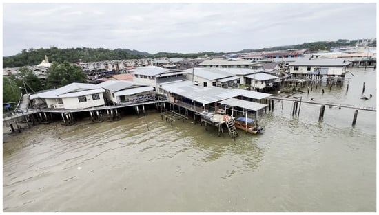
Figure 1.
Traditional stilt village (Kampong Ayer) in Sungai Brunei.
The river is a gaining river divided into two main sections: the upper reaches, which provide freshwater to the western regions of the country [2], and the lower reaches, which function as a breeding ground for coastal fisheries. The river is flanked by extensive mangroves and interwoven with a labyrinth of interconnecting channels that ultimately discharge into Brunei Bay towards the northeast direction. As the Brunei River approaches Brunei Bay, its lower reaches transition into an estuarine system strongly influenced by tides. The river experiences a semidiurnal tidal regime [43] from the South China Sea, with a daily tidal range fluctuating between 1 and 2.5 m. Tidal intrusion extends upstream, altering water levels, salinity, and flow direction in the lower river [3]. During high tides, seawater can penetrate several kilometers inland, creating a brackish environment that impacts the river’s self-purification capacity. Along its course, the river receives additional water flow from several tributaries, including the Damuan, Butir, Kedayan, and Kianggeh rivers, contributing to its flow and water composition. The river’s catchment primarily consists of alluvial deposits overlying the Belait Formation [12] while the landscape features a mix of low-lying swampy plains, peat swamp forests, and hilly terrain.
Brunei’s climate, shaped by equatorial monsoon winds, significantly influences the river’s hydrology. The northeast monsoon dominates from December to March, while the southwest monsoon occurs from May to September, with transitional periods in April, October, and November. The region experiences its primary peak in rainfall from October to January, with December being the wettest month. A secondary rainfall peak occurs from May to July, notably in May, while the driest periods extend from late January to March and from late July to September. Temperatures remain warm year-round, ranging from 28 °C to 32 °C [44], and total annual rainfall exceeds 2300 mm throughout the country.
Despite its ecological significance, the lower stretches of the Brunei River face substantial pollution challenges. The primary sources of contamination include untreated sewage effluent and stormwater runoff, especially from areas surrounding Bandar Seri Begawan and Kampong Ayer. During the rainy seasons, these pollution levels are exacerbated by surface runoff, which transports contaminants from both urban and agricultural areas into the river.
- Data Collection
Eight monitoring stations (B, D, E, G, J, N, P, Q) were strategically selected along the Brunei River (coordinates: 4°52′–4°56′ N, 114°54′–115°0′ E) based on their proximity to both point source and non-point source pollution areas (Figure 2).
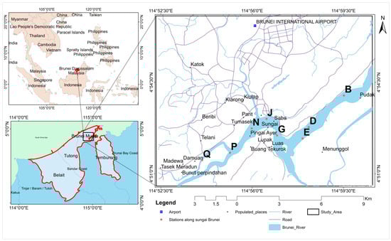
Figure 2.
Location map of the study area.
These stations were chosen to capture a comprehensive understanding of the river’s water quality, focusing on areas that are heavily impacted by urban, agricultural, and residential activities contributing to pollution. The data for this study were collected from September 2013 to June 2022. Population data for the study period were obtained from the Department of Economic Planning and Statistics, Ministry of Finance and Economy, Brunei. Coliform bacteria data concentrations were collected and quantified using a multiple tube fermentation approach [45] at the wastewater laboratory of the Department of Drainage and Sewerage (DDS), Public Works Department, Brunei Darussalam.
- Data Transformation
To ensure the data conformed to normality, a log transformation was applied. Given the non-normal distribution of the continuous time series coliform data, the transformation was necessary to normalize the data and improve the validity of statistical analyses [46]. This approach helps reduce skewness and ensures the data fit the assumptions required for more robust statistical tests. In addition to normalizing the data, the log transformation was employed to mitigate the influence of extreme values or outliers. Using the log to base 10 (log10) transformation, the data became less sensitive to extreme variations, allowing for a more accurate and stable analysis of the coliform bacteria concentrations [47]. This step ensures that very high or low values do not disproportionately affect the overall analysis.
- Box plot
Box plots were used to visually summarize data distributions, showing key statistics: minimum, Q1, median, Q3, and maximum values [48]. The interquartile range (IQR) captures data variability, while whiskers and outliers show the spread and unusual values, respectively.
- Propensity Score Matching (PSM)
Propensity score matching (PSM) was used to assess the causal relationship between population growth and coliform bacteria concentrations across the eight monitoring stations along the Brunei River. PSM is a statistical technique designed to estimate the effect of a treatment, in this case, high population growth, by matching observations from treated and untreated groups based on their propensity to experience the treatment [35]. This method reduces selection bias in observational data and simulates conditions akin to a randomized controlled experiment. To isolate the impact of high population growth, time periods were categorized into two groups: high population growth (the treatment group) and low/no population growth (the control group). The top 25% of months, based on population growth rate, were designated as the treatment group, while the bottom 25% were designated as the control group. Once treated and control observations were identified based on the actual population growth data, propensity scores were then calculated for both groups. The propensity score represents the probability that a time period would experience high population growth, estimated using Logistic Regression with coliform bacteria concentrations from each station (Q, G, J, N, P, B, D, and E) as covariates. The Logistic Regression equation used to calculate the propensity is shown in Equation (1) below:
where P (High Growth) is the probability of a time period having high population growth, β0 represents the intercept, and βi represent the regression coefficients for the coliform concentrations Ci at the respective stations i∈ {Q, G, J, N, P, B, D, E}. logit( ) represents the logit function, which is the natural logarithm of the odds of an event occurring. After propensity scores were calculated, the time periods were sorted by propensity scores. Matching was performed using the nearest neighbor matching method [49,50] by comparing the highest propensity score periods (high population growth) with the lowest propensity score periods (low/no population growth). This process created balanced treatment and control groups that were similar in terms of their baseline coliform concentrations but differed in their population growth status. After matching, we compared the average coliform bacteria concentrations between the high and low population growth groups to estimate the causal effect of population growth. The average treatment effect (ATT) on the treated group was calculated as the difference in coliform concentrations between the matched groups (Equation (2)):
where Nτ is the number of matched time periods, Yi High Growth represents the coliform concentration in the high growth group, and Yi Low Growth represents the coliform concentration in the matched low growth group.
- Rescaled Adjusted Partial Sums (RAPS) Analysis
To evaluate the temporal evolution and structural shifts in coliform bacteria concentrations, this study employed the Rescaled Adjusted Partial Sums (RAPS) method. RAPS is a robust statistical technique that enables the detection of cumulative deviations from the mean, effectively highlighting long-term trends, episodic shifts, and stochastic fluctuations within a time series [36,51]. Unlike parametric trend analysis methods that assume linearity, RAPS accounts for both gradual changes and abrupt anomalies, making it well suited for analyzing microbial contamination in aquatic systems.
The RAPS series was computed using the following transformation (Equation (3)):
where RAPSi is the Rescaled Adjusted Partial Sum at time step i, xj is the value of the observed coliform bacteria concentration at time step j, is the mean of the entire time series dataset, is standard deviation of the dataset, i is time step, and j is the index of summation from 1 to i. By rescaling observations relative to their statistical dispersion, this approach effectively amplifies deviations from the mean, allowing for the identification of underlying trends and inflection points that might otherwise remain undetected in raw time series data. Furthermore, a monotonic increase in RAPS values indicates a persistent upward trend in coliform concentrations, whereas a declining trajectory suggests an overall improvement in water quality.
- Time Series and Trend Analysis of the Total Coliform Bacteria
- Long Short-Term Memory (LSTM)
- (1)
- Data Preprocessing
For total coliform future prediction and trends, we first employed a Long Short-Term Memory (LSTM) model, a type of recurrent neural network (RNN) specifically designed to capture long-term dependencies in time series data [52]. LSTM models are well suited for time series forecasting because of their ability to retain information over extended sequences, making them ideal for modeling sequential data where past values may influence future outcomes. Coliform time series data from the eight stations (B, D, E, G, J, N, P, and Q) underwent comprehensive preprocessing. MinMaxScaler was applied to normalize the data to a range between 0 and 1, optimizing the performance of the LSTM model [53]. This normalization is a critical step for improving the convergence of the LSTM model during training.
- (2)
- Data Augmentation
Given the limited size of our data set (106 data points for each station), data augmentation (Figure 3) techniques were applied to increase the training data, thus improving the model’s generalization capabilities. Jittering introduced slight variations in the data by adding small amounts of random noise, with a standard deviation of 0.01, to the original time series. This technique augmented the training set by simulating additional data points with minor variability, enhancing the model’s robustness. Additionally, a sliding window approach was implemented, where each window consisted of 60 time steps, with the output variable being the value immediately following each window. This allowed the model to capture temporal dependencies over 60 months of data, and the resulting sequences were used as input for training. The original and jitter-augmented datasets were then combined, effectively doubling the training set, thus providing the model with a larger sample size to learn from and improving its ability to capture the patterns and dynamics of coliform fluctuations.
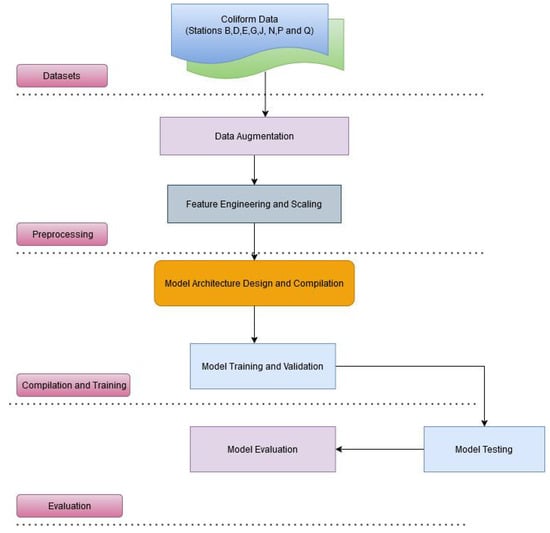
Figure 3.
Long Short-Term model for the eight monitoring stations (B, D, E, G, J, N, P, and Q).
- (3)
- Model Architecture
The Bidirectional LSTM (BiLSTM) network was then employed to capture both past and future dependencies in the time series data. The input layer was defined as a sequence of 60 time steps derived from the rolling windows, with each sequence treated as univariate time series data. Two stacked Bidirectional LSTM layers were used, with the first layer consisting of 64 units that returned sequences for further processing and the second layer composed of 32 units that returned only the last time step for prediction. A dropout rate of 0.2 was applied after each LSTM layer, randomly deactivating 20% of the neurons during training to prevent overfitting. Finally, a fully connected dense layer with a single neuron was utilized as the output layer to predict the next coliform level in the sequence.
- (4)
- Training and Evaluation
Furthermore, during the training process, early stopping was implemented to ensure efficient training by preventing overfitting, with the dataset split into approximately 70% for training, 20% for validation, and 10% for testing. The model was trained using the Adam optimizer [54] and the Mean Squared Error (MSE) loss function, with batch training conducted on 16 samples per batch. Although the model was set to train for a maximum of 1000 epochs, early stopping frequently terminated training earlier to enhance performance. After training, the model was evaluated on both the training and test sets using four key metrics [55]: Mean Absolute Error (MAE), which measures the average absolute difference between predictions and actual values; Mean Squared Error (MSE), assessing the average squared difference with an emphasis on more significant errors; Root Mean Squared Error (RMSE), which provides error in the same units as the target variable; and R-squared (R2), explains how much of the variance in coliform levels is captured by the model. Finally, a learning curve was plotted during the training process to visualize how the model’s performance improved over time. The learning curve illustrated the loss (error) on both the training and validation sets over the course of the training epochs. This provided insight into the model’s convergence behavior, showing how quickly the model learned the underlying patterns in the data and whether or not it overfitted. The curve was analyzed to ensure that the model’s validation loss decreased steadily without divergence from the training loss, confirming that the early stopping mechanism worked effectively. The trained model was then used to make predictions for coliform levels over the next five years, while Mann–Kendall was used for detecting significant monotonic or declining trends of the total coliform time series data [56].
- Autoregressive Integrated Moving Average (ARIMA)
We also utilized the Autoregressive Integrated Moving Average (ARIMA) model to forecast coliform concentrations for the next five years across eight monitoring stations (B, D, E, G, J, N, P, and Q). Time series data for each station, spanning from September 2013 to June 2022, were preprocessed to ensure temporal consistency and completeness. Each station’s dataset was sorted and split into training (80%) and testing (20%) subsets. Stationarity was assessed using the Augmented Dickey–Fuller test [36], and differencing was applied where necessary to stabilize the series. The ARIMA model parameters (p, d, and q) for each station were determined through autocorrelation and partial autocorrelation analysis [36], with the best-fitting model selected for each dataset. The models were fitted to the training data, and testing data forecasts were generated for validation. Performance metrics, including the Mean Absolute Error (MAE), Mean Squared Error (MSE), Root Mean Squared Error (RMSE), and R-squared, were calculated to evaluate predictive accuracy. Using the validated models, 60-month forecasts were generated for each station, representing the expected coliform concentrations over the next five years. Future dates were created to align with the forecast horizon, and the results were plotted alongside historical data to visualize trends and assess potential future water quality risks at each station.
- Logistic Regression
Logistic Regression was used to forecast coliform concentrations at eight monitoring stations (B, D, E, G, J, N, P, and Q) over a 5-year period, using time series data from September 2013 to June 2022. The dataset for each station was sorted by date, and a lag feature representing the previous observation was created to serve as the predictor variable [37]. Missing values resulting from this lag operation were removed to ensure data consistency. The data were split into training and testing subsets, with 80% allocated for training the model and 20% reserved for testing and validation. Logistic Regression models were developed for each station, with the lagged coliform values as the independent variable and the observed concentrations as the dependent variable. The models were trained on the historical data and validated using the testing subset. Model performance was evaluated using metrics such as Mean Absolute Error (MAE), Mean Squared Error (MSE), Root Mean Squared Error (RMSE), and R-squared (R2) to assess accuracy and generalization. Future forecasts for the next 60 months were generated using a recursive approach [37], where each new prediction served as input for the subsequent forecast.
3. Results and Discussion
The two box plots (Figure 4a,b) present a comparative analysis of total coliform concentrations across the eight sampling sites during the rainy and dry seasons. For this study, February, March, April, August, and September were categorized as the dry season. These months typically experience fewer rainy days and lower overall precipitation levels. In contrast, January, May, June, July, October, November, and December were categorized as the rainy season.
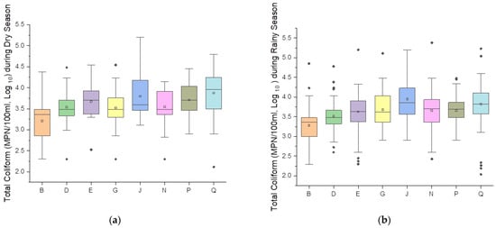
Figure 4.
Seasonal variations in total coliform levels in the Brunei River during dry (a) and wet (b) seasons from September 2013 to June 2022. The dash line represents the median, the inner squares represent the mean while extreme values are the outliers.
Upstream Station Q recorded maximum TC concentrations of 5.23 MPN/100 mL, log10 during the rainy season compared to 4.79 MPN/100 mL, log10 in the dry season. This increase can be attributed to agricultural and quarry runoff, which intensifies during rainfall due to the mobilization of sediments and fecal matter from nearby residential areas [20,57]. Similarly, Station P, located near agricultural zones, showed a maximum of 4.48 in the rainy season compared to 4.45 MPN/100 mL, log10 in the dry season, despite the presence of natural buffers like mangrove forests around Station P; the proximity of nearby anthropogenic activities led to persistent coliform bacteria pollution.
The water village (Kampong Ayer) Stations N and J experienced significant seasonal variations due to the combined impacts of untreated direct sewage discharge and stormwater runoff. At Station N, coliform concentrations peaked at 5.38 during the rainy season, compared to 4.15 MPN/100 mL, log10 in the dry season. Station J recorded elevated values of 5.20 MPN/100 mL, log10 in both the rainy and dry season. These results align with studies linking runoff to episodic spikes in microbial contamination during rainfall events [15]. The consistent presence of coliform bacteria during the dry season reflects baseline contamination from point sources, a pattern commonly observed in many waterways with inadequate wastewater management [58]. Upstream Station G also recorded a maximum TC concentration of 5.11 MPN/100 mL, log10 during the rainy season compared to 4.54 MPN/100 mL, log10 in the dry season.
Downstream Station E, near the Pintu Malim Sewage Treatment Plant, recorded a rainy season maximum of 5.20 MPN/100 mL, log10 compared to 4.54 MPN/100, log10 in the dry season. While the treatment facility likely mitigates dry season pollution, the cumulative upstream contributions during rainfall events may have overwhelmed its capacity. These findings are consistent with studies detailing the limitations of treatment infrastructure in mitigating stormwater-induced pollution [59,60]. Downstream Stations D and B showed relatively stable seasonal patterns, reflecting the influence of natural dilution and tidal flushing. At Station D, the maximum TC level increased slightly from 4.48 in the dry season to 4.78 (MPN/100 mL, log10) in the rainy season, while at Station B, it rose from 4.38 to 4.85 (MPN/100 mL, log10). These results show the role of estuarine processes in moderating coliform levels, a phenomenon also observed in other tidal river systems [61,62]. However, the elevated rainy season maxima could indicate the cumulative impact of upstream pollution transported during precipitation events. Notably, the observed coliform bacteria concentrations exceed the water quality standards set by the USEPA [63] and Malaysia [64] for both drinking water and recreational activities.
- Impact of Population Growth on the Total Coliform Bacteria
Water pollution is a growing concern across many Asian countries, where rapid urbanization has outpaced the development of essential infrastructure such as sewerage and water supply systems [65]. In this study, propensity score matching (PSM) was used to assess the impact of population growth on coliform bacteria concentrations across the eight monitoring stations along the Brunei River. The Average Treatment Effect on the Treated (ATT) (Figure 5) illustrates the spatial variations in the response of coliform concentrations to population growth across the eight monitoring stations along the Brunei River. Station J experienced the highest increase in coliform concentrations during periods of high population growth. This station is located at the interface between Bandar Seri Begawan (capital city) and Kampong Ayer (water village), an area subject to significant domestic pollution due to its high population density. The rise in coliform levels at Station J is likely attributed to untreated direct sewage discharge and runoff from nearby urban infrastructure, particularly from the densely populated city center. These findings align with previous research, which has demonstrated that population growth in rapidly urbanizing areas is often accompanied by increased fecal contamination in nearby water bodies due to inadequate wastewater management and overflow from combined sewer systems [26].
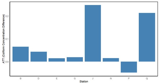
Figure 5.
Average Treatment Effect on the Treated (ATT) for coliform concentrations at eight monitoring stations (B, D, E, G, J, N, P, and Q) along the Brunei River.
Station Q also showed a substantial increase in coliform levels, though slightly lower than Station J (Figure 5). This station is located upstream from Bandar Seri Begawan, near the confluence of Sungai Damuan with Sungai Brunei, and is surrounded by residential areas, agricultural land, and a quarry. The elevated ATT value at Station Q indicates that runoff from nearby residential areas contributes to increased coliform bacteria levels. This is likely a result of poorly maintained or inadequately designed drainage systems, which lack the necessary hydraulic capacity to manage stormwater effectively [65]. Consequently, the area experiences river discoloration and odor issues due to the accumulation of contaminants in the water bodies. In contrast, Station P, located in a largely forested agricultural area, showed a decrease in coliform concentrations during periods of population growth, as indicated by its negative ATT (Figure 5). Stations B, D, G, and N exhibited minimal changes in coliform concentrations in response to population growth, suggesting that these areas are less affected by population growth. Station E showed a near-zero ATT, indicating almost no difference in coliform concentrations between periods of high and low population growth.
- Overall Trend Analysis of Coliform Contamination in Sungai Brunei
The temporal trends in coliform bacteria concentrations across Sungai Brunei using the RAPS method showed significant shifts in microbial water quality over the observed period. Between 2013 and 2018 (Figure 6a–h), a sustained decline in coliform levels was evident across the eight monitoring stations, which may be attributed to multiple factors, including low population and rainfall around the study area during this period and the natural self-purification capacity of the river. A critical transition in the coliform bacteria emerged between 2018 and 2019, marking a shift from declining to increasing coliform levels.
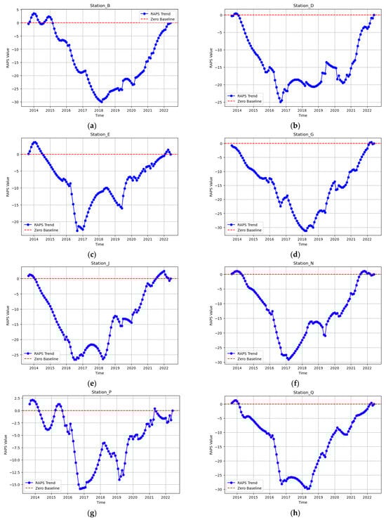
Figure 6.
(a–h) RAPS trend at the eight monitoring stations from 2013 to 2022.
This inflection point suggests that underlying pressures on water quality intensified, leading to a deterioration in microbial conditions across the river system. The reversal in the declining trend is likely associated with increased urbanization and anthropogenic pressures, particularly in upstream stations experiencing a rapid expansion of impervious surfaces [66,67,68,69] and the direct discharge of fecal matter into the river. The failure or overburdening of existing sewage treatment facilities, coupled with increasing wastewater discharge into the river, may have exacerbated coliform contamination [70,71,72]. In populated areas like Kampong Ayer and Bandar Seri Begawan, Stations N and J saw significant contamination spikes, likely due to rising sewage discharge, deteriorating sanitation infrastructure, and direct wastewater disposal from stilt house settlements. Further downstream, Station G initially showed a decline in coliform levels but later followed the broader post-2018 increase due to urban expansion and stormwater inputs [20]. At Station E, near the Pintu Malim Sewage Treatment Plant, microbial levels stabilized until 2018 but then surged, raising concerns about treatment efficiency and the plant’s capacity to handle increasing wastewater volumes. Stations D and B had a delayed response, with rising coliform concentrations becoming evident in later years. Initially buffered by estuarine mixing, Station B eventually showed sustained increases, suggesting upstream pollution loads now exceed natural purification processes, posing risks to coastal water quality and marine ecosystems.
- ARIMA, Logistic Regression, and BiLSTM predictions
The forecasting of total coliform concentrations for the next five years was conducted using ARIMA, Logistic Regression, and BiLSTM models (Figure 7, Figure 8 and Figure 9) for eight monitoring stations (B, D, E, G, J, N, P, and Q) in the Brunei River.
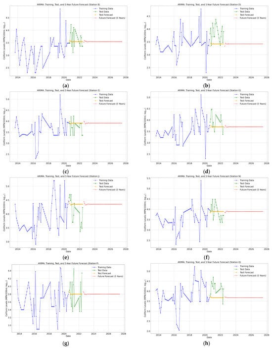
Figure 7.
(a–h) ARIMA 5-year future predictions of total coliform bacteria in the Brunei River.
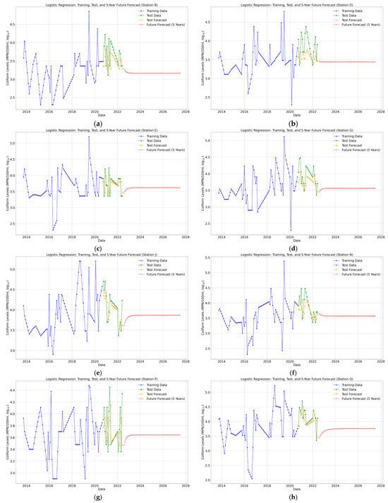
Figure 8.
(a–h) Logistic Regression 5-year future predictions of total coliform bacteria in the Brunei River.
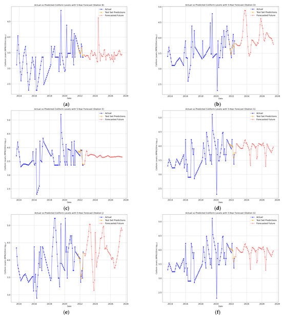
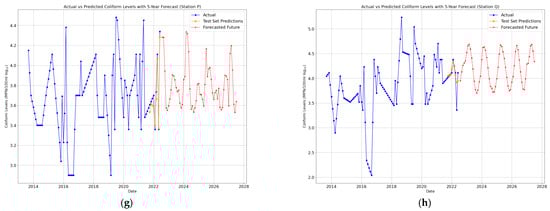
Figure 9.
(a–h) BiLSTM 5-year future predictions of total coliform bacteria in the Brunei River.
Each model was chosen for its ability to analyze and predict temporal trends of a small dataset. ARIMA utilized the historical patterns and seasonality in the time series, Logistic Regression relied on lagged features to predict coliform levels, and BiLSTM leveraged deep learning to model non-linear relationships and capture long-term dependencies. Furthermore, key performance metrics (Figure 10a–d) and Table A1, Table A2 and Table A3 (see Appendix A), including Mean Absolute Error (MAE), Mean Squared Error (MSE), Root Mean Squared Error (RMSE), and R-squared (R2), were compared to evaluate the models’ accuracies across each monitoring station.
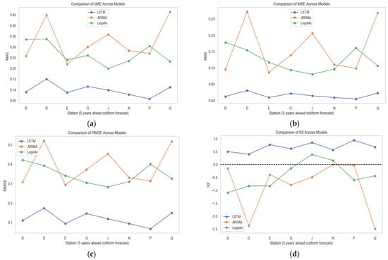
Figure 10.
(a–d) Model estimation using MAE, MSE, RMSE, and R-squared.
BiLSTM consistently demonstrated superior performance (Figure 10), achieving the lowest MAE across all stations. This suggests that BiLSTM, with its unique ability to capture complex temporal dependencies in the coliform dataset, leads to more precise forecasts [73]. Conversely, ARIMA recorded the highest MAE values, indicating its inadequacy in accurately predicting coliform levels [74]. While marginally outperforming ARIMA, Logistic Regression still showed relatively high MAE values, reinforcing its limitations in time series forecasting. Moreover, examining the MSE values further underscores the efficiency of BiLSTM. The model consistently produced the lowest MSE, reflecting its ability to mitigate significant forecasting errors. ARIMA, on the other hand, exhibited the highest MSE, signifying substantial deviations in its predictions of the coliform levels in the monitoring stations. Logistic Regression performed better than ARIMA in this regard but still lagged behind BiLSTM, confirming the deep learning model’s dominance in water quality forecasting [52,53,54,55].
Furthermore, the RMSE findings align with the trends observed in the MSE (Figure 10b). BiLSTM consistently achieved the lowest RMSE across all stations, indicating minimal deviations from observed values. In contrast, ARIMA’s predictions resulted in the highest RMSE values, reinforcing its tendency to generate substantial errors [74,75,76,77] in a small dataset. Logistic Regression fared slightly better but remained significantly less accurate than BiLSTM [78]. In addition, the R2 values provide additional insight into model efficacy. A high R2 value indicates a model’s ability to explain variance within the dataset. BiLSTM outperformed ARIMA and Logistic Regression by achieving the highest R2 values across all stations, confirming its ability to capture coliform trends effectively. ARIMA, however, consistently returned negative R2 values, demonstrating its inability to model coliform fluctuations adequately. A negative R2 value indicates that the model does not follow the trend of the data, which is a significant limitation in forecasting. Logistic Regression produced mixed results, with predominantly negative R2 values, except at Station J, where a slight positive correlation was observed.
When analyzing model behavior across different stations, BiLSTM consistently delivered a superior performance, with good results at Stations E, J, and P, where error values were significantly lower and R2 values were higher. This suggests that BiLSTM is well suited for stations with stable yet dynamic coliform bacteria patterns. ARIMA exhibited its poorest performance at Stations B, D, and N, where it failed to capture coliform-level fluctuations and produced the highest error values. Logistic Regression performed inconsistently, showing relatively improved performance at Stations J and G but failing to provide reliable forecasts at Stations B, D, and P. Station Q displayed moderate error values across all models, suggesting that none fully captured its underlying patterns.
The overall comparison clearly establishes BiLSTM as the most reliable and accurate model for long-term coliform forecasting in a small dataset. With its lowest error rates and highest R2 values, BiLSTM emerges as the optimal choice for predicting coliform levels over a 5-year horizon, showcasing its potential for long-term forecasting. ARIMA struggles significantly, with its significant errors and negative R2 values indicating poor model fit. While moderately better than ARIMA, Logistic Regression still fails to provide sufficiently accurate predictions, limiting its applicability in coliform forecasting. Given these findings, BiLSTM is strongly recommended for long-term coliform forecasting due to its superior accuracy and predictive capability. These findings align with the established strengths of deep learning models in handling complex temporal relationships [52,55], reinforcing their suitability for dynamic environmental systems. The challenges faced by ARIMA and Logistic Regression reflect their reliance on simpler linear relationships and limited feature representations, which are less effective in heterogeneous and variable environments like the Brunei River.
Since the BiLSTM model consistently outperformed ARIMA and Logistic Regression across all stations, the Mann–Kendall trend analysis was applied to the next five years of predicted data. The analysis revealed a significant upward trend at the 0.05 significance level for Stations B, D, E, G, J, N, and Q, indicating that gradual increases in total coliform concentrations in the Brunei River over time may be attributed to urbanization, population growth, and the direct discharge of wastewater into the river. In contrast, Station P showed no significant upward trend at the 0.05 level, highlighting the need for continued monitoring to identify potential shifts that could emerge over a longer timeframe. To mitigate the growing coliform contamination in the Brunei River, strengthening wastewater treatment infrastructure is essential to reduce microbial pollution from sewage discharge. The effective regulation of sewer and septic tank overflows is necessary to prevent fecal contamination, particularly in densely populated (Kampong Ayer) regions. Additionally, the enforcement of stricter land use policies can minimize agricultural runoff, thereby reducing coliform inputs from livestock waste and fertilizers.
4. Conclusions and Future Outlook
This study addresses the challenges of total coliform bacteria concentrations in the Brunei River. Despite the small dataset, the box plot findings reveal significant increases in total coliform concentrations during the rainy season across urban and agricultural zones, coupled with persistent baseline contamination during the dry season, which shows the vulnerability of the Brunei River to anthropogenic activities. Propensity score matching showed that population growth exacerbates contamination, particularly at the water village, where inadequate wastewater infrastructure contributes to higher pollution levels. The RAPS analysis revealed an increase in microbial water quality post-2018, driven by urban expansion, increased impervious surfaces, and escalating sewage discharge. Although estuarine mixing initially mitigated contamination, the growing pollution load has surpassed the river’s natural purification.
Among the models employed, BiLSTM demonstrated remarkable results, achieving an R2 > 0.7 in most stations. Its ability to capture non-linear patterns and long-term dependencies proved critical in overcoming data limitations. In contrast, ARIMA and Logistic Regression were less effective, as their reliance on simpler relationships made them unsuitable for the variability and complexity of the Brunei River’s pollution. The Mann–Kendall trend analysis applied to the BiLSTM-predicted data for the next five years revealed significant upward trends in coliform levels at most stations (B, D, E, G, J, N, and Q), emphasizing the growing impact of urbanization, population growth, and direct wastewater discharge in the Brunei River. In contrast, Station P, situated in an agricultural area, revealed no significant upward trend, suggesting a relatively stable pollution pattern. These findings emphasize the critical need for targeted mitigation strategies to address localized pollution sources, particularly in urban and residential zones, while advocating for ongoing monitoring efforts to detect emerging trends in areas currently showing stability.
Furthermore, this study shows the potential of advanced machine learning models in data-scarce environments, where traditional methods often fall short. However, addressing data limitations remains imperative. Expanding monitoring networks, increasing sampling frequency, and integrating auxiliary data sources, such as land use and meteorological data, can enhance model accuracy and reliability. These efforts will support the development of effective water quality management strategies for the Brunei River and similar tropical river systems facing the dual pressures of population growth and climatic variability. Future research should explore hybrid models combining BiLSTM with other advanced deep learning techniques, such as graph neural networks (GNNs) or Transformers, to enhance forecasting accuracy and robustness.
Author Contributions
Conceptualization, O.O. and S.H.G.; methodology, O.O. and Z.K.L.; software, O.O. and Z.K.L.; validation, N.S., O.O., Z.K.L., P.E.A., D.T.C.L. and S.H.G.; formal analysis, O.O.; investigation, O.O. and S.H.G.; resources, O.O., Z.K.L. and S.H.G.; data curation, O.O.; writing—original draft preparation, O.O.; writing—review and editing, O.O., Z.K.L., P.E.A., D.T.C.L. and S.H.G.; visualization, O.O. and Z.K.L.; supervision, N.S., D.T.C.L., P.E.A. and S.H.G.; project administration, O.O. and S.H.G.; funding acquisition, N.S., S.H.G. and D.T.C.L. All authors have read and agreed to the published version of the manuscript.
Funding
Universiti Brunei Darussalam, research grant UBD/RSCH/1.18/FICBF(b)/2022/004.
Data Availability Statement
Data are not publicly available but can be made available based on reasonable requests to the corresponding authors.
Acknowledgments
The authors thank the Public Works Department of Brunei Darussalam for the supplied data.
Conflicts of Interest
The authors declare no conflicts of interest.
Appendix A

Table A1.
BiLSTM model.
Table A1.
BiLSTM model.
| Station | MAE | MSE | RMSE | R-Squared |
|---|---|---|---|---|
| B | 0.09 | 0.0124 | 0.1115 | 0.5039 |
| D | 0.1505 | 0.0306 | 0.1749 | 0.4043 |
| E | 0.0868 | 0.0091 | 0.0955 | 0.7731 |
| G | 0.1153 | 0.0217 | 0.1471 | 0.6165 |
| J | 0.0985 | 0.0144 | 0.1201 | 0.8565 |
| N | 0.0781 | 0.0091 | 0.0953 | 0.5749 |
| P | 0.0572 | 0.0048 | 0.0692 | 0.9473 |
| Q | 0.1116 | 0.0226 | 0.1504 | 0.6796 |
Table A2.
Logistic Regression model.
Table A2.
Logistic Regression model.
| Station | MAE | MSE | RMSE | R-Squared |
|---|---|---|---|---|
| B | 0.334963 | 0.177972 | 0.421868 | −1.0882 |
| D | 0.337138 | 0.154356 | 0.392881 | −0.82851 |
| E | 0.239556 | 0.116899 | 0.341905 | −0.82927 |
| G | 0.260403 | 0.093035 | 0.305016 | −0.14876 |
| J | 0.199122 | 0.080381 | 0.283516 | 0.394807 |
| N | 0.235115 | 0.096349 | 0.310401 | 0.159552 |
| P | 0.304635 | 0.160779 | 0.400972 | −0.59889 |
| Q | 0.232499 | 0.106417 | 0.326215 | −0.43631 |
Table A3.
ARIMA model.
Table A3.
ARIMA model.
| Station | MAE | MSE | RMSE | R-Squared |
|---|---|---|---|---|
| B | 0.258089 | 0.095371 | 0.308822 | −0.14994 |
| D | 0.449202 | 0.271895 | 0.521436 | −2.3706 |
| E | 0.219562 | 0.086307 | 0.293781 | −0.38696 |
| G | 0.29977 | 0.138721 | 0.372452 | −0.79203 |
| J | 0.358228 | 0.206121 | 0.454006 | −0.48849 |
| N | 0.283008 | 0.109868 | 0.331464 | −0.00195 |
| P | 0.269625 | 0.098471 | 0.3138 | −0.02138 |
| Q | 0.46467 | 0.267888 | 0.517579 | −2.48897 |
References
- Ismail, R.; Suhaili, W.S.; Patchmuthu, R.K. IoT Based Water Quality Monitoring in Relation to Flood and Drought in Brunei Darussalam. In Proceedings of the 2023 13th International Conference on Information Technology in Asia (CITA), Samarahan, Malaysia, 3–4 August 2023; pp. 54–59. [Google Scholar] [CrossRef]
- Azffri, S.L.; Azaman, A.; Sukri, R.S.; Jaafar, S.M.; Ibrahim, M.F.; Schirmer, M.; Gödeke, S.H. Soil and Groundwater Investigation for Sustainable Agricultural Development: A Case Study from Brunei Darussalam. Sustainability 2022, 14, 1388. [Google Scholar] [CrossRef]
- Onifade, O.; Shamsuddin, N.; Lai, D.T.C.; Jamil, H.; Gödeke, S.H. Importance of baseline assessments: Monitoring of Brunei River’s water quality. H2Open J. 2023, 6, 518–534. [Google Scholar] [CrossRef]
- Gӧdeke, S.H.; Malik, O.A.; Lai, D.T.C.; Bretzler, A.; Schirmer, M.; Mansor, N.H. Water quality investigation in Brunei Darussalam: Investigation of the influence of climate change. Environ. Earth Sci. 2020, 79, 419. [Google Scholar] [CrossRef]
- Shams, S.; Reza, M.S.; Azad, A.K.; Juani, R.B.H.M.; Fazal, M.A. Environmental Flow Estimation of Brunei River Based on Climate Change. Environ. Urban. ASIA 2021, 12, 257–268. [Google Scholar] [CrossRef]
- Ogwu, M.C.; Pamela, B.O.; Ayilara, F.D.; Kurotimipa, F.O.; Adams, O.I. Traditional and Conventional Water Treatment Methods: A Sustainable Approach. Water Crises and Sustainable Management in the Global South; Springer Nature Singapore: Singapore, 2024; pp. 461–486. [Google Scholar] [CrossRef]
- Yang, Q.; Chen, J.; Dai, J.; He, Y.; Wei, K.; Gong, M.; Chen, Q.; Sheng, H.; Su, L.; Liu, L.; et al. Total coliforms, microbial diversity and multiple characteristics of Salmonella in soil-irrigation water-fresh vegetable system in Shaanxi, China. Sci. Total Environ. 2024, 924, 171657. [Google Scholar] [CrossRef]
- Procopio, N.A.; Atherholt, T.B.; Goodrow, S.M.; Lester, L.A. The Likelihood of Coliform Bacteria in NJ Domestic Wells Based on Precipitation and Other Factors. Groundwater 2017, 55, 722–735. [Google Scholar] [CrossRef]
- Seo, M.; Lee, H.; Kim, Y. Relationship between Coliform bacteria and water quality factors at weir stations in the Nakdong River, South Korea. Water 2019, 11, 1171. [Google Scholar] [CrossRef]
- Bohra, D.L.; Modasiya, V.; Bahura, C.K. Distribution of coliform bacteria in waste water. Microbiol. Res. 2012, 3, 2. [Google Scholar] [CrossRef]
- Food and Agricultural Organization (FAO). Manuals of food quality control: Microbiological analysis. In Food and Nutrition Paper; Food and Agricultural Organization: Rome, Italy, 1979. [Google Scholar]
- Onifade, O.; Shamsuddin, N.; Jin, J.L.Z.; Lai, D.T.C.; Gödeke, S.H. Assessment of Pollution Status in Brunei River Using Water Quality Indices, Brunei Darussalam. Water 2024, 16, 2493. [Google Scholar] [CrossRef]
- Sehgal, S.; Aggarwal, S.; Banik, S.P.; Kaushik, P. Impact of Water Contamination on Food Safety and Related Health Risks. In Microbial Biotechnology in the Food Industry; Springer International Publishing: Berlin/Heidelberg, Germany, 2024; pp. 337–363. [Google Scholar] [CrossRef]
- Haile, R.W.; Witte, J.S.; Gold, M.; Cressey, R.; Mcgee, C.; Millikan, R.C.; Glasser, A.; Harawa, N.; Ervin, C.; Harmon, P.; et al. The Health Effects of Swimming in Ocean Water Contaminated by Storm Drain Runoff. Epidemiology 1999, 10, 355–363. [Google Scholar]
- Singh, A.K.; Das, S.; Singh, S.; Pradhan, N.; Gajamer, V.R.; Kumar, S.; Lepcha, Y.D.; Tiwari, H.K. Physicochemical parameters and alarming coliform count of the potable water of Eastern Himalayan state Sikkim: An indication of severe fecal contamination and immediate health risk. Front. Cell Dev. Biol. 2019, 7, 174. [Google Scholar] [CrossRef] [PubMed]
- You, S.; Huang, X.; Xing, L.; Lesperance, M.; LeBlanc, C.; Moccia, L.P.; Mercier, V.; Shao, X.; Pan, Y.; Zhang, X. Dynamics of fecal coliform bacteria along Canada’s coast. Mar. Pollut. Bull. 2023, 189, 114712. [Google Scholar] [CrossRef]
- Santos, N.G.N.; Silva, L.C.; Guidone, G.H.M.; Montini, V.H.; Oliva, B.H.D.; Nascimento, A.B.; de Sousa, D.N.R.; Kuroda, E.K.; Rocha, S.P.D. Water quality monitoring in southern Brazil and the assessment of risk factors related to contamination by coliforms and Escherichia coli. J. Water Health 2023, 21, 1550–1561. [Google Scholar] [CrossRef] [PubMed]
- Leong, S.S.; Ismail, J.; Denil, N.A.; Sarbini, S.R.; Wasli, W.; Debbie, A. Microbiological and physicochemical water quality assessments of riverwater in an industrial region of the northwest coast of Borneo. Water 2018, 10, 1648. [Google Scholar] [CrossRef]
- Gautam, B.; Kasi, M.; Lin, W. Determination of Fecal Coliform Loading and its Impact on River Water Quality for TMDL Development. Proc. Water Environ. Fed. 2006, 9, 3851–3874. [Google Scholar] [CrossRef]
- Ahmed, W.; Hamilton, K.; Toze, S.; Cook, S.; Page, D. A review on microbial contaminants in stormwater runoff and outfalls: Potential health risks and mitigation strategies. Sci. Total Environ. 2019, 692, 1304–1321. [Google Scholar] [CrossRef]
- Xu, K.; Valeo, C.; He, J.; Xu, Z. Climate and land use influences on bacteria levels in stormwater. Water 2019, 11, 2451. [Google Scholar] [CrossRef]
- Chigbu, P.; Gordon, S.; Strange, T.R. Fecal coliform bacteria disappearance rates in a north-central Gulf of Mexico estuary. Estuarine, Coast. Shelf Sci. 2005, 65, 309–318. [Google Scholar] [CrossRef]
- Karunakaran, E.; Battarbee, R.; Tait, S.; Beltran, B.M.; Berney, C.; Grinham, J.; Herrero, M.A.; Omolo, R.; Douterelo, I. Integrating molecular microbial methods to improve faecal pollution management in rivers with designated bathing waters. Sci. Total Environ. 2024, 912, 168565. [Google Scholar] [CrossRef]
- Harris, C.S.; Tertuliano, M.; Rajeev, S.; Vellidis, G.; Levy, K. Impact of storm runoff on Salmonella and Escherichia coli prevalence in irrigation ponds of fresh produce farms in southern Georgia. J. Appl. Microbiol. 2018, 124, 910–921. [Google Scholar] [CrossRef]
- Bodus, B.; O’Malley, K.; Dieter, G.; Gunawardana, C.; McDonald, W. Review of emerging contaminants in green stormwater infrastructure: Antibiotic resistance genes, microplastics, tire wear particles, PFAS, and temperature. Sci. Total Environ. 2024, 906, 167195. [Google Scholar] [CrossRef] [PubMed]
- Olds, H.T.; Corsi, S.R.; Dila, D.K.; Halmo, K.M.; Bootsma, M.J.; McLellan, S.L. High levels of sewage contamination released from urban areas after storm events: A quantitative survey with sewage specific bacterial indicators. PLoS Med. 2018, 15, e1002614. [Google Scholar] [CrossRef] [PubMed]
- Tornevi, A.; Bergstedt, O.; Forsberg, B. Precipitation effects on microbial pollution in a river: Lag structures and seasonal effect modification. PLoS ONE 2014, 9, e98546. [Google Scholar] [CrossRef]
- Ayejoto, D.; Egbueri, J.C.; Agbasi, C.A.; Omeka, M.E.; Unigwe, O.C.; Nwazelibe, V.E.; Ighalo, O.J.; Pande, B.C. Influence of Seasonal Changes on the Quality of Water Resources in Southwestern Nigeria: A Review. In Climate Change Impacts on Nigeria 2023; Springer: Cham, Switzerland, 2023. [Google Scholar] [CrossRef]
- Buckerfield, S.J.; Quilliam, R.S.; Waldron, S.; Naylor, L.A.; Li, S.; Oliver, D.M. Rainfall-driven E. coli transfer to the stream-conduit network observed through increasing spatial scales in mixed land-use paddy farming karst terrain. Water Res. X 2019, 5, 100038. [Google Scholar] [CrossRef]
- Kaihena, M.; Talakua, C.M.; Pagaya, J.; Talakua, S.M. Analysis of water pollution in microbiology aspect of some watersheds at Ambon City, Maluku Province. IOP Conf. Ser. Earth Environ. Sci. 2021, 805, 012021. [Google Scholar] [CrossRef]
- Liyanage, C.P.; Yamada, K. Impact of population growth on the water quality of natural water bodies. Sustainability 2017, 9, 1405. [Google Scholar] [CrossRef]
- World Bank. World Development Indicators. Available online: https://data.worldbank.org/indicator/SP.POP.TOTL?locations=BN (accessed on 5 September 2023).
- Hasan, N.A.; Ratnayake, U.; Shams, S. Evaluation of rainfall and temperature trends in Brunei Darussalam. Am. Inst. Phys. Conf. Proc. 2016, 1705, 020034. [Google Scholar] [CrossRef]
- Oluwaniyi, O.; Zhang, Y.; Gholizadeh, H.; Li, B.; Gu, X.; Sun, H.; Lu, C. Correlating Groundwater Storage Change and Precipitation in Alabama, United States from 2000–2021 by Combining the Water Table Fluctuation Method and Statistical Analyses. Sustainability 2023, 15, 15324. [Google Scholar] [CrossRef]
- Langworthy, B.; Wu, Y.; Wang, M. An overview of propensity score matching methods for clustered data. Stat. Methods Med. Res. 2023, 32, 641–655. [Google Scholar] [CrossRef]
- Šrajbek, M.; Đurin, B.; Sušilović, P.; Singh, S.K. Application of the RAPS Method for Determining the Dependence of Nitrate Concentration in Groundwater on the Amount of Precipitation. Earth 2023, 4, 266–277. [Google Scholar] [CrossRef]
- Zafra-Mejía, C.A.; Rondón-Quintana, H.A.; Urazán-Bonells, C.F. ARIMA and TFARIMA Analysis of the Main Water Quality Parameters in the Initial Components of a Megacity’s Drinking Water Supply System. Hydrology 2024, 11, 10. [Google Scholar] [CrossRef]
- Choi, S.Y.; Seo, I.W. Prediction of fecal coliform using logistic regression and tree-based classification models in the North Han River, South Korea. J. Hydro-Environ. Res. 2018, 21, 96–108. [Google Scholar] [CrossRef]
- Lawal, Z.K.; Yassin, H.; Teck Ching Lai, D.; Che Idris, A. Understanding the Dynamics of Ocean Wave-Current Interactions Through Multivariate Multi-Step Time Series Forecasting. Appl. Artif. Intell. 2024, 38, 2393978. [Google Scholar] [CrossRef]
- Niknam, A.R.R.; Sabaghzadeh, M.; Barzkar, A.; Shishebori, D. Comparing ARIMA and various deep learning models for long-term water quality index forecasting in Dez River, Iran. Environ. Sci. Pollut. Res. 2024, 805, 012021. [Google Scholar] [CrossRef]
- Mohan Tito Ayyalasomayajula, M. Innovative Water Quality Prediction for Efficient Management Using Ensemble Learning. Educ. Adm. Theory Pract. 2023, 29, 2374–2381. [Google Scholar] [CrossRef]
- Abbas, A.; Baek, S.; Silvera, N.; Soulileuth, B.; Pachepsky, Y.; Ribolzi, O.; Boithias, L.; Cho, K.H. In-stream Escherichia coli modeling using high-temporal-resolution data with deep learning and process-based models. Hydrol. Earth Syst. Sci. 2021, 25, 6185–6202. [Google Scholar] [CrossRef]
- Marshall, D.; Proum, S.; Hossain, M.B.; Adam, A.; Lim, L.H.; Santos, J.H. Ecological responses to fluctuating and extreme marine acidification: Lessons from a tropical estuary (the Brunei Estuarine System). Sci. Bruneiana 2016, 15, 1–12. [Google Scholar] [CrossRef]
- Chua, T.E.; Chou, L.M.; Sadorra, M.S.M. The Coastal Environmental Profile of Brunei Darussalam: Resource Assessment and Management Issues, ICLARM Technical Reports. In Fisheries Department, Ministry of Development, Brunei Darussalam and International Center for Living Aquatic Resources Management, Manila, Philippines; ICLARM: Manila, Philippines, 1987; Volume 18, p. 193. [Google Scholar]
- APHA. Standard Methods for the Examination of Water and Wastewater. In American Public Health Association, American Water Works Association, 20th ed.; Water Pollution Control Facility Joint Publications: Washington, DC, USA, 1995. [Google Scholar]
- Feng, C.; Wang, H.; Lu, N.; Chen, T.; He, H.; Lu, Y.; Tu, X.M. Log-transformation and its implications for data analysis. Shanghai Arch. Psychiatry 2014, 26, 105–109. [Google Scholar] [CrossRef]
- Ayach, M.; Lazar, H.; Bousouis, A.; Touiouine, A.; Kacimi, I.; Valles, V.; Barbiero, L. Multi-Parameter Analysis of Groundwater Resources Quality in the Auvergne-Rhône-Alpes Region (France) Using a Large Database. Resources 2023, 12, 143. [Google Scholar] [CrossRef]
- Dawson, R. How significant is a boxplot outlier? J. Stat. Educ. 2011, 19, 2. [Google Scholar] [CrossRef]
- Randolph, J.; Falbe, K. A Step-by-Step Guide to Propensity Score Matching in R. Pract. Assess. Res. Eval. 2014, 19, 18. [Google Scholar]
- Austin, P.C. An introduction to propensity score methods for reducing the effects of confounding in observational studies. Multivar. Behav. Res. 2011, 46, 399–424. [Google Scholar] [CrossRef] [PubMed]
- Bonacci, O.; Trninić, D.; Roje-Bonacci, T. Analysis of the water temperature regime of the Danube and its tributaries in Croatia. Hydrol. Process. Int. J. 2008, 22, 1014–1021. [Google Scholar] [CrossRef]
- Hochreiter, S.; Schmidhuber, J. Long short-term memory. Neural Computation 1997, 9, 1735–1780. [Google Scholar] [CrossRef]
- Sembiring, I.; Wahyuni, S.N.; Sediyono, E. LSTM algorithm optimization for COVID-19 prediction model. Heliyon 2024, 10, e26158. [Google Scholar] [CrossRef]
- Gholizadeh, H.; Zhang, Y.; Frame, J.; Gu, X.; Green, C.T. Long short-term memory models to quantify long-term evolution of streamflow discharge and groundwater depth in Alabama. Sci. Total Environ. 2023, 901, 165884. [Google Scholar] [CrossRef]
- Khullar, S.; Singh, N. Water quality assessment of a river using deep learning Bi-LSTM methodology: Forecasting and validation. Environ. Sci. Pollut. Res. 2022, 29, 12875–12889. [Google Scholar] [CrossRef]
- Gocic, M.; Trajkovic, S. Analysis of changes in meteorological variables using Mann-Kendall and Sen’s slope estimator statistical tests in Serbia. Glob. Planet. Change 2013, 100, 172–182. [Google Scholar] [CrossRef]
- Monteiro, S.; Queiroz, G.; Ferreira, F.; Santos, R. Characterization of stormwater runoff based on microbial source tracking methods. Front. Microbiol. 2021, 12, 674047. [Google Scholar] [CrossRef]
- Makuwa, S.; Tlou, M.; Fosso-Kankeu, E.; Green, E. The effects of dry versus wet season on the performance of a wastewater treatment plant in North West Province, South Africa. Water SA 2022, 48, 40–49. [Google Scholar] [CrossRef]
- Burns, M.J.; Fletcher, T.D.; Walsh, C.J.; Ladson, A.R.; Hatt, B.E. Hydrologic shortcomings of conventional urban stormwater management and opportunities for reform. Landsc. Urban Plan. 2012, 105, 230–240. [Google Scholar] [CrossRef]
- Sinigalliano, C.D.; Gidley, M.L.; Shibata, T.; Whitman, D.; Dixon, T.H.; Laws, E.; Hou, A.; Bachoon, D.; Brand, L.; Amaral-Zettler, L.; et al. Impacts of Hurricanes Katrina and Rita on the microbial landscape of the New Orleans area. Proc. Natl. Acad. Sci. USA 2007, 104, 9029–9034. [Google Scholar] [CrossRef]
- Ketchum, B.H.; Ayers, J.C.; Vaccaro, R.F. Processes Contributing to the Decrease of Coliform Bacteria in a Tidal Estuary. Ecology 1952, 33, 247–258. [Google Scholar] [CrossRef]
- Muhtadi, A.; Leidonald, R.; Fadhilah, A. Water Quality Dynamics and Water Pollutions of Belawan Estuary, North Sumatra-Indonesia. North Sumatra-Indones. 2024. [Google Scholar] [CrossRef]
- U.S. Environmental Protection Agency. Quality Criteria for Water; U.S. Environmental Protection Agency: Washington, DC, USA, 1976; EPA-440976023.
- Department of Environment. *National Water Quality Standards and Water Quality Index*. Available online: https://www.doe.gov.my/en/national-river-water-quality-standards-and-river-water-quality-index/ (accessed on 28 March 2025).
- Kazmi, A.; Furumai, H. Sustainable urban wastewater management and reuse in Asia. Int. Rev. Environ. Strateg. 2005, 5, 425–448. [Google Scholar]
- Asowata, I.T.; Badejo, O.O.; Onifade, O.M.; Olukoya, F.F. Spatial distribution of trace element of Ala river’s sediments, Akure, Southwestern Nigeria. Ife J. Sci. 2015, 17, 109–120. [Google Scholar]
- Vitro, K.A.; BenDor, T.K.; Jordanova, T.V.; Miles, B. A geospatial analysis of land use and stormwater management on fecal coliform contamination in North Carolina streams. Sci. Total Environ. 2017, 603, 709–727. [Google Scholar] [CrossRef]
- Abidin, H.; Azffri, S.L.; Nirus, E.; Suhip, A.; Jaya, A.A.; Gödeke, S.H. Groundwater mapping of urban and coastal areas in Brunei. J. Water Land Dev. 2024, 61, 21–29. [Google Scholar] [CrossRef]
- Oluwaniyi, O.E.; Asiwaju-Bello, Y.A. Geochemical processes influencing stream water chemistry: A case study of Ala River, Akure, Southwestern Nigeria. Sustain. Water Resour. Manag. 2020, 6, 108. [Google Scholar] [CrossRef]
- Xiao, S.; Hu, S.; Zhang, Y.; Zhao, X.; Pan, W. Influence of sewage treatment plant effluent discharge into multipurpose river on its water quality: A quantitative health risk assessment of Cryptosporidium and Giardia. Environ. Pollut. 2018, 233, 797–805. [Google Scholar] [CrossRef]
- Ullah Bhat, S.; Qayoom, U. Implications of Sewage Discharge on Freshwater Ecosystems. IntechOpen 2022, 1–18. [Google Scholar] [CrossRef]
- Xie, Y.; Liu, X.; Wei, H.; Chen, X.; Gong, N.; Ahmad, S.; Taeho, L.; Ismail, S.; Ni, S.Q. Insight into impact of sewage discharge on microbial dynamics and pathogenicity in river ecosystem. Sci. Rep. 2022, 12, 6894. [Google Scholar] [CrossRef]
- Pyo, J.; Pachepsky, Y.; Kim, S.; Abbas, A.; Kim, M.; Kwon, Y.S.; Ligaray, M.; Cho, K.H. Long short-term memory models of water quality in inland water environments. Water Res. X 2023, 21, 100207. [Google Scholar] [CrossRef] [PubMed]
- Siami-Namini, S.; Tavakoli, N.; Namin, A.S. A comparison of ARIMA and LSTM in forecasting time series. In Proceedings of the 2018 17th IEEE International Conference on Machine Learning and Applications (ICMLA), Orlando, FL, USA, 17–20 December 2018; pp. 1394–1401. [Google Scholar]
- Zaini, N.A.; Ean, L.W.; Ahmed, A.N.; Abdul Malek, M.; Chow, M.F. PM2. 5 forecasting for an urban area based on deep learning and decomposition method. Sci. Rep. 2022, 12, 17565. [Google Scholar] [CrossRef]
- Gajewski, P.; Čule, B.; Rankovic, N. Unveiling the Power of ARIMA, Support Vector and Random Forest Regressors for the Future of the Dutch Employment Market. J. Theor. Appl. Electron. Commer. Research. 2023, 18, 1365–1403. [Google Scholar] [CrossRef]
- Al-Najjar, H.; Ceribasi, G.; Dogan, E.; Qahman, K.; Abualtayef, M.; Ceyhunlu, A.I. Statistical modeling of spatial and temporal vulnerability of groundwater level in the Gaza Strip (Palestine). H2Open J. 2021, 4, 352–365. [Google Scholar] [CrossRef]
- Heyer, T.; Stamm, J. Levee reliability analysis using logistic regression models–abilities, limitations and practical considerations. Georisk Assess. Manag. Risk Eng. Syst. Geohazards 2013, 7, 77–87. [Google Scholar] [CrossRef]
Disclaimer/Publisher’s Note: The statements, opinions and data contained in all publications are solely those of the individual author(s) and contributor(s) and not of MDPI and/or the editor(s). MDPI and/or the editor(s) disclaim responsibility for any injury to people or property resulting from any ideas, methods, instructions or products referred to in the content. |
© 2025 by the authors. Licensee MDPI, Basel, Switzerland. This article is an open access article distributed under the terms and conditions of the Creative Commons Attribution (CC BY) license (https://creativecommons.org/licenses/by/4.0/).