Analysis of Prediction Confidence in Water Quality Forecasting Employing LSTM

Abstract

Water quality prediction serves as an important foundation for risk control and the proactive management of the aquatic environment, and the Long Short-Term Memory (LSTM) network has gained recognition as an effective approach for achieving high-precision water quality predictions. However, despite its potential, there is a significant gap in the literature regarding the confidence analysis of its prediction accuracy and the underlying causes of variability across different water quality indicators and basins. To address this gap, the present study introduces a novel confidence evaluation method to systematically assess the performance of LSTM in predicting key water quality parameters, including ammonia nitrogen (AN), biochemical oxygen demand (BOD), chemical oxygen demand (COD), dissolved oxygen (DO), hydrogen ion concentration (pH), and total phosphorus (TP). This evaluation was conducted across three basins with distinct geographical, climatic, and water quality conditions: the Huangshui River Basin (HSB), the Haihe River Basin (HRB), and the Yangtze River Basin (YRB). The results of the confidence evaluation revealed that LSTM exhibited higher credibility in the Haihe River Basin compared to the Yangtze River Basin. Additionally, LSTM demonstrated greater accuracy and stability in predicting total phosphorus (TP) compared to other water quality indicators in both basins, with median NSE values of 0.71 in the HRB and 0.73 in the YRB. Additionally, the research demonstrated a linear relationship between the ability of LSTM models to predict the water quality and temporal autocorrelation as well as the cross-correlation coefficients of the water quality parameters. The coefficients of determination (R²) ranged from 0.59 to 0.85, with values of 0.59 and 0.79 for the YRB and 0.85 and 0.80 for the HRB, respectively. This finding underscores the importance of considering these correlation metrics when evaluating the reliability of LSTM-based predictions.

1. Introduction

Over the past few decades, artificial intelligence (AI) has emerged as an effective alternative approach for modeling complex nonlinear systems [1]. Extensive research has been conducted on river water quality prediction, monitoring, and management using various AI models, including artificial neural networks (ANNs) [1,2,3,4], adaptive neuro-fuzzy inference systems (ANFISs) [5,6,7], and support vector machines (SVMs) [8,9], among others. However, recurrent neural networks (RNNs) are particularly well suited for sequential data due to their inherent structure [10], and they have been utilized for water quality prediction [11,12]. The Long Short-Term Memory (LSTM) network addresses the vanishing or exploding gradient issues associated with RNNs [13], making it even more effective for handling sequential data, such as water quality information [10,14]. Recently, LSTM-based models have demonstrated promising performance in water quality prediction [14,15,16,17,18,19,20].

Recent studies have demonstrated that Long Short-Term Memory (LSTM) networks hold significant value in many time-series predictions and exhibit excellent simulation capabilities. For instance, in the field of runoff prediction, LSTM models have been shown to provide accurate and reliable results, especially when combined with time-frequency analysis methods. However, it is crucial to recognize that LSTM models have their own limitations and are not universally applicable. They are designed to handle specific types of sequential data and may not perform well in all scenarios. For example, the Root Mean Square Errors (RMSEs) of LSTM models for dissolved oxygen (DO) differ across various basins: 0.0396 in Jiangsu Wuxi of the Yangtze River, China; 0.55 in the Prespa Basin in southeastern Europe; 0.07 in Tai Lake, China; and 0.067 in Victoria Bay, China [14,15,21]. Similarly, within the same basin, LSTM models exhibit different performances for various indicators. In the Beilun Estuary of the Guangxi Autonomous Region, China, the Mean Absolute Errors (MAEs) for predicting the weekly pH, DO, chemical oxygen demand (COD), and ammonia nitrogen (AN) were 0.58, 0.51, 0.71, and 0.68, respectively [20]. Moreover, the performance of LSTM is influenced by various factors, including data characteristics, model parameters, and training methods. Despite these considerations, there is a notable gap in the literature regarding the credibility analysis of LSTM predictions. While numerous studies have focused on comparing different models or incrementally improving existing ones, there is a lack of in-depth research on evaluating the confidence level of LSTM predictions in diverse applications [1,18]. For example, in water quality prediction, LSTM models show varying performances across different basins and indicators. The Root Mean Square Errors (RMSEs) of LSTM models for dissolved oxygen (DO) differ significantly across various basins: 0.04 in Jiangsu Wuxi of the Yangtze River, China; 0.545 in the Prespa Basin in southeastern Europe; 0.07 in Tai Lake, China; and 0.067 in Victoria Bay, China [22,23]. Similarly, within the same basin, LSTM models exhibit different performances for various indicators. In the Beilun Estuary of the Guangxi Autonomous Region, China, the Mean Absolute Errors (MAEs) for predicting the weekly pH, DO, chemical oxygen demand (COD), and ammonia nitrogen (AN) were 0.58, 0.51, 0.71, and 0.68, respectively [23,24,25]. However, the underlying causes of these variations remain largely unexplored. There is a striking deficiency in the literature regarding the feasibility and applicability of data-driven models for various water quality indicators and across diverse basins. Although it is evident that LSTM performance fluctuates with different indicators and basins, the root causes of these discrepancies remain largely unexplored. The absence of comprehensive credibility analysis significantly hampers the reliable application and broader adoption of LSTM models in practical scenarios.

The Yangtze River Basin (YRB), the Haihe River Basin (HRB), and the Huangshui River Basin (HSB) are three different basins with distinctive features in China, located in the southern, northern, and northwestern regions, respectively. The YRB is characterized by its humid climate, abundant rainfall, and rich water resources, whereas the HRB is relatively dry, with scarce water resources and frequent water shortages [18,26,27,28,29]. It is worth highlighting that the Haihe River Basin (HRB) experiences the most critical levels of water scarcity and pollution when compared to the other six major river basins in China [30]. Accurate water quality forecasts are essential for early warning and timely intervention to mitigate pollution in these basins [31]. The water shortage problem is more serious in the HSB; the water quantity is scarce, and the water pollution level is serious [32]. Various models, including process-based and machine learning models, have been applied to predict water quality in the HRB [18,33,34,35,36,37] and YRB [21,38,39,40,41]. However, LSTM-based models have been underutilized in these regions [18,21]. Moreover, LSTM applications have been limited to predicting the dissolved oxygen (DO) in both basins, while other critical pollution indicators, such as the biochemical oxygen demand (BOD) and total phosphorus (TP), urgently need to be assessed. Further research is needed to analyze the prediction accuracy of LSTM for these additional water quality indicators. Additionally, comparative analysis of LSTM performance in areas with different water resource availability and pollution conditions is essential to evaluate its applicability.

Comparing LSTM performance between the HRB and YRB can not only reveal the characteristics and influencing factors of LSTM in different regions but also provide valuable insights for similar studies worldwide. As a result, an analytical comparison of the effectiveness of water quality forecasting using LSTM models was conducted across the Yangtze and Haihe River Basins. Our aims are twofold: (1) to demonstrate the diverse performance of LSTM in predicting water quality across different basins and elucidate the underlying causes and (2) to establish the connection between LSTM performance and the data characteristics of the modeled region.

2. Methodology

2.1. Study Area

The Yangtze River Basin (YRB), Haihe River Basin (HRB), and Huangshui River Basin (HSB) were selected as the study area (shown in Figure 1).

The YRB is the largest river in China and the third longest river in the world [42,43,44]. Most of the YRB is in the subtropical monsoon climate zone [29] and is characterized by a warm/humid climate but with an irregular distribution of annual average temperature and precipitation in both the spatial and temporal dimensions. The Haihe River is the largest river catchment in Northern China [45].

The Haihe River Basin (HRB) has about 1.05 × 10⁵ m³/km² (less than one-fifth of that in the YRB) of water resources, covering an area of about 2.6 × 10⁵ km². Located in a continental monsoon climate zone, the HRB belongs to semi-humid and semi-arid region [46]. With the rapid urbanization and economic development, the HRB receives large amount of sewage and waste discharged from varied origins [45,47]. Accordingly, the HRB suffers the most water shortages and water pollution among all seven river basins in China.

The Huangshui River Basin (HSB) plays a crucial role in the socio-economic advancement of Qinghai Province, China. However, due to its typical alpine and arid climate, the basin faces significant challenges, including drought, water shortages, and soil erosion. The average annual precipitation in the HSB ranges from 300 to 500 mm, while the average annual evaporation rate is as high as 800 to 1500 mm, indicating a severe water scarcity situation [30].

2.2. Data Sources

The water quality dataset encompasses monthly records for 23 monitoring sites within the Yangtze River Basin (YRB) spanning from 2003 to 2018, 76 monitoring sites in the Huai River Basin (HRB) from 2010 to 2020, and 68 monitoring sites in the Huangshui River Basin (HSB) between 2011 and 2021 (Figure 1). The monthly concentrations for biochemical oxygen demand (BOD), chemical oxygen demand (COD), dissolved oxygen (DO), ammonia nitrogen (AN), total phosphorus (TP), and hydrogen ion concentration (pH) were collected.

The mean, minimum, maximum, standard deviation (SD), and coefficient of variation (CV) were used for a comparative evaluation of model performance in the three basins, as shown in

Table 1. Basic statistical analysis for water quality indicators of three basins.

Basins	Indicators	Unit	Mean	Minimum	Maximum	SD	CV
YRB	AN	mg/L	0.178	0.025	1.340	0.184	1.035
	BOD	mg/L	1.100	0.500	2.500	0.400	0.300
	COD	mg/L	2.200	0.500	4.100	0.500	0.200
	DO	mg/L	8.530	4.400	13.10	1.510	0.180
	pH	-	7.970	6.930	8.920	0.330	0.040
	TP	mg/L	0.072	0.005	0.250	0.051	0.706
HRB	AN	mg/L	8.104	0.012	122.00	14.554	1.796
	BOD	mg/L	12.300	0.200	220.00	24.700	2.000
	COD	mg/L	11.000	0.600	127.00	16.00	1.400
	DO	mg/L	6.750	0.020	18.80	3.500	0.520
	pH	-	7.890	6.420	8.990	0.380	0.050
	TP	mg/L	0.730	0.005	8.880	1.243	1.703
HSB	AN	mg/L	0.572	0.011	10.80	0.929	1.622
	BOD	mg/L	2.100	0.200	24.00	1.700	0.800
	COD	mg/L	2.100	0.200	13.00	1.000	0.500
	DO	mg/L	8.190	3.220	12.700	1.200	0.150
	pH	-	8.220	6.490	9.290	0.310	0.040
	TP	mg/L	0.081	0.005	1.190	0.103	1.270

.

The Maximal Information Coefficient (MIC) can be utilized as a versatile tool for detecting and quantifying complex dependencies between variables, going beyond traditional correlation measures, which often fail to capture nonlinear relationships [48]. The MIC was computed and employed to determine both temporal autocorrelation and cross-correlation coefficients for water quality indicators across various lag periods, ranging from 1 to 12 months, as illustrated in Figure 2. The measurement MIC is symmetric and normalized into a range $\left[0,1\right]$. A high MIC value indicates a strong dependency between the investigated variables, whereas MIC = 0 describes the relationship between two independent variables.

2.3. Model Development Based on LSTM Models

2.3.1. Principle of the Model

As an advanced recurrent neural network (RNN), Long Short-Term Memory (LSTM) has a specialized neuron structure. This neuron structure has a selective memory function [14,49] by means of a special model structure design, a memory block, for information filtering and conversion [16,50]. A memory block is composed of a forget gate, an input gate, a memory cell, and an output gate [13,51], with its state at a given time depicted in Figure 3.

In the Long Short-Term Memory (LSTM) model, at the preceding time step (t − 1), the memory block retains crucial information in the form of both the cell state (C_t−1) and the output (h_t−1). The initial values for the cell state (C₀) and the hidden state (h₀) are typically set to zero, serving as the starting point for the LSTM cell’s memory. As it progresses to time step t, the current inputs (X_t) become accessible. The process begins with deriving the hidden state (h_t) through a nonlinear transformation. This transformation utilizes the output gate and the newly updated cell state, as described in Equation (1). This hidden state (h_t) encapsulates the information learned from the previous time steps and the current input, forming the basis for subsequent calculations. Next, four multi-layer perceptrons (MLPs) are employed to compute key gates and states within the LSTM cell. Specifically, these MLPs are formulated as Equations (2)–(4) and (6), and they calculate the forget gate (f_t), the candidate cell state ($\widetilde{c_t})$, the input gate (i_t), and the output gate (o_t). These calculations are based on the previous hidden state (h_t−1) and the current input (X_t). The forget gate (f_t) decides what information to discard from the previous cell state, the input gate (i_t) determines what new information to add, and the candidate cell state ($\widetilde{c_t})$ represents the potential new values for the cell state. The output gate (o_t) controls the output based on the updated cell state. Finally, the updated cell state (C_t) is calculated using the relationship outlined in Equation (5). This new cell state incorporates the forgotten information, the new input, and any other modifications decided by the gates, effectively updating the LSTM cell’s memory for the current time step.

$$h_t=o_t\ast {tanh(c}_t)$$

(1)

$$f_t=\sigma \left(W_{xf}{X}_t+W_{hf}{h}_{t-1}+b_f\right)$$

(2)

$$\widetilde{c_t}=\mathit{tanh}\left(W_{xc}{X}_t+W_{hc}{h}_{t-1}+b_c\right)$$

(3)

$$i_t=\sigma \left(W_{xi}{X}_t+W_{hi}{h}_{t-1}+b_t\right)$$

(4)

$$c_t=f_t\ast c_{t-1}+i_t\ast \widetilde{c_t}$$

(5)

$$o_t=\sigma \left(W_{xo}{X}_t+W_{ho}{h}_{t-1}+b_0\right)$$

(6)

In Equations (2)–(4) and (6), $W$ denotes the matrices of weights for the gates or cells with the corresponding subscripts, and $b$ represents learnable biases. Additionally, $\sigma$ and $tanh$ denote the sigmoid function and the tanh function, respectively.

Long Short-Term Memory (LSTM) networks are powerful tools in the realm of deep learning, distinguished by their ability to retain and manipulate information over extended temporal periods. By incorporating specialized memory cells, LSTM networks can “remember” the most pertinent input values, making them exceptionally well suited for sequential learning tasks [49]. This capability enables LSTM models to capture long-term dependencies and patterns within data sequences, which is crucial for accurate predictions and understanding of temporal dynamics.

In the context of the present study, LSTM models were meticulously developed to forecast future one-month values of a specific water quality indicator. To achieve this, two distinct configurations of input variables were employed:

(1) Univariate inputs: In this configuration, the LSTM models solely rely on historical data of the targeted water quality indicator. This approach is straightforward and focuses on understanding the temporal evolution of the single variable of interest.

(2) Multivariate inputs: Alternatively, the LSTM models were also trained using historical data from all available water quality indicators. This multivariate approach provides a more comprehensive view of the water quality system, potentially capturing interdependencies and correlations between different indicators.

For both input configurations, the time steps (k) for the model inputs were varied from 1 to 12 months. This means that the LSTM models were fed with time-series data spanning from the previous 1 to k months.

2.3.2. Model Training and Testing

The data from each station were randomly divided into three subsets—80% for training, 10% for validation, and 10% for testing—to facilitate model training. And same kind of subsets from the same basin were combined to form the training, validation, and test dataset. Then, all water quality indicators were standardized according to Equation (1) to ensure that the model’s input variables remained on the same scale and to guarantee a stable convergence of parameters in LSTM [52].

$$\widetilde{x_i}={\displaystyle \frac{x_i-\overline{x}}{std}}$$

(7)

Here, $\overline{x}$ and $std$ signify the average and standard deviation of the training dataset, respectively; $x_i$ defines every single value of the raw data, while $\widetilde{x_i}$ represents the standardized value.

2.3.3. Model Optimization

For each LSTM model, Keras Tuner (https://keras-team.github.io/keras-tuner/, accessed on 31 March 2025) was employed to optimize the model hyperparameters via a 150-time random search (10 repetitive times training for each random search) from the searching space of hidden layers and neurons [53]. Other hyperparameters of LSTM were determined using trial and error. The batch size and the dropout rates were 256 and 0.5, respectively. The maximum number of epochs for model training was established at 200, signifying that the training phase would terminate when convergence was reached or when the 200 predefined epochs had elapsed. Furthermore, an initial learning rate of 0.1 was assigned to facilitate the learning process. This rate undergoes automatic adjustment downwards if there is no notable improvement in the loss function on the validation dataset for five straight epochs.

During the training phase, models are developed using the training dataset, with Keras Tuner being instrumental in pinpointing the best model architectures through thorough performance assessments on the validation dataset. After identifying these optimal architectures, the LSTM models are fine-tuned through a retraining process and subsequently assessed on both training and testing datasets. To mitigate the variability caused by the random initialization of model parameters, the entire cycle of training, optimization, retraining, and evaluation is carefully repeated 100 times, ensuring the creation of robust, reliable, and generalizable LSTM models.

2.4. Confidence Analysis of LSTM Models

In the field of deep learning and machine learning, confidence is an important measure of the predictive reliability of a model and a key factor in determining whether a model is usable. Confidence usually refers to the degree to which a model is certain of its predictions, and this degree of confidence can be quantified. The applicability of the LSTM model is a key issue that needs to be evaluated for practical application scenarios, such as watershed water quality prediction. Although LSTM performs well in many time-series prediction tasks, its scope of application is limited and cannot be arbitrarily applied to all scenarios. Therefore, this paper constructs a set of model confidence evaluation methods.

2.4.1. Model Accuracy Calculation

By comparing the predicted value and the real value, the accuracy of the model base on the Nash–Sutcliffe Efficiency (NSE; Equation (8)) [50] will be judged. The Nash–Sutcliffe Efficiency (NSE; Equation (8)) [50], a widely recognized metric for hydrological model evaluation [2,51], is employed as the model assessment criterion in the current study:

$$NSE=1-{\displaystyle \frac{{\sum }_{i=1}^n{\left(y_{m,i}-y_{p,i}\right)}^2}{{\sum }_{i=1}^n{\left(y_{m,i}-\overline{y_m}\right)}^2}}$$

(8)

where n is the number of observations; $y_{m,i}$ and $y_{p,i}$ define the ith observations and the corresponding values predicted using LSTM, respectively; and $\overline{y_m}$ represents the average of observations. In a lot of studies, the NSE ranges from $-\mathrm{\infty }$ to 1. The model is acceptable when the NSE ≥ 0.60 [54] and good when the NSE ≥ 0.75 [2,55].

2.4.2. Confidence Analysis

The confidence level and confidence interval were used for confidence analysis based on the NSE. The confidence value under confidence level Z is:

$$c_Z=\overline{X}\pm {\displaystyle \frac{Z\times \sigma }{\sqrt{n}}}$$

(9)

The confidence coefficient, defined as $\delta$, can be simulated as:

$$\delta =max(0,\overline{X}-d_Z)$$

(10)

$$d_Z={\displaystyle \frac{max\left(c_Z\right)-min\left(c_Z\right)}{max\left(c_Z\right)}}$$

(11)

where $\overline{X}$ is the mean of the NSE, $\sigma$ is the standard deviation, n is the sample size, $Z$ is the coefficient under the confidence level (usually 95%), and $d_Z$ is the confidence width of the confidence interval under Z. According to the accuracy evaluation basis of the NSE, the classification criteria are divided into four levels and determined as follows:

$$L\delta =\left\{\begin{array}{cc}L1& bad, \delta <0.4\\ L2& acceptable, 0.4\le \delta <0.6\\ \begin{array}{c}L3\\ L4\end{array}& \begin{array}{c}\begin{array}{cc}& good,\end{array} 0.6\le \delta <0.7\\ \begin{array}{cc}& excellent\end{array},\delta \ge 0.7\end{array}\end{array}\right.$$

(12)

3. Results and Discussion

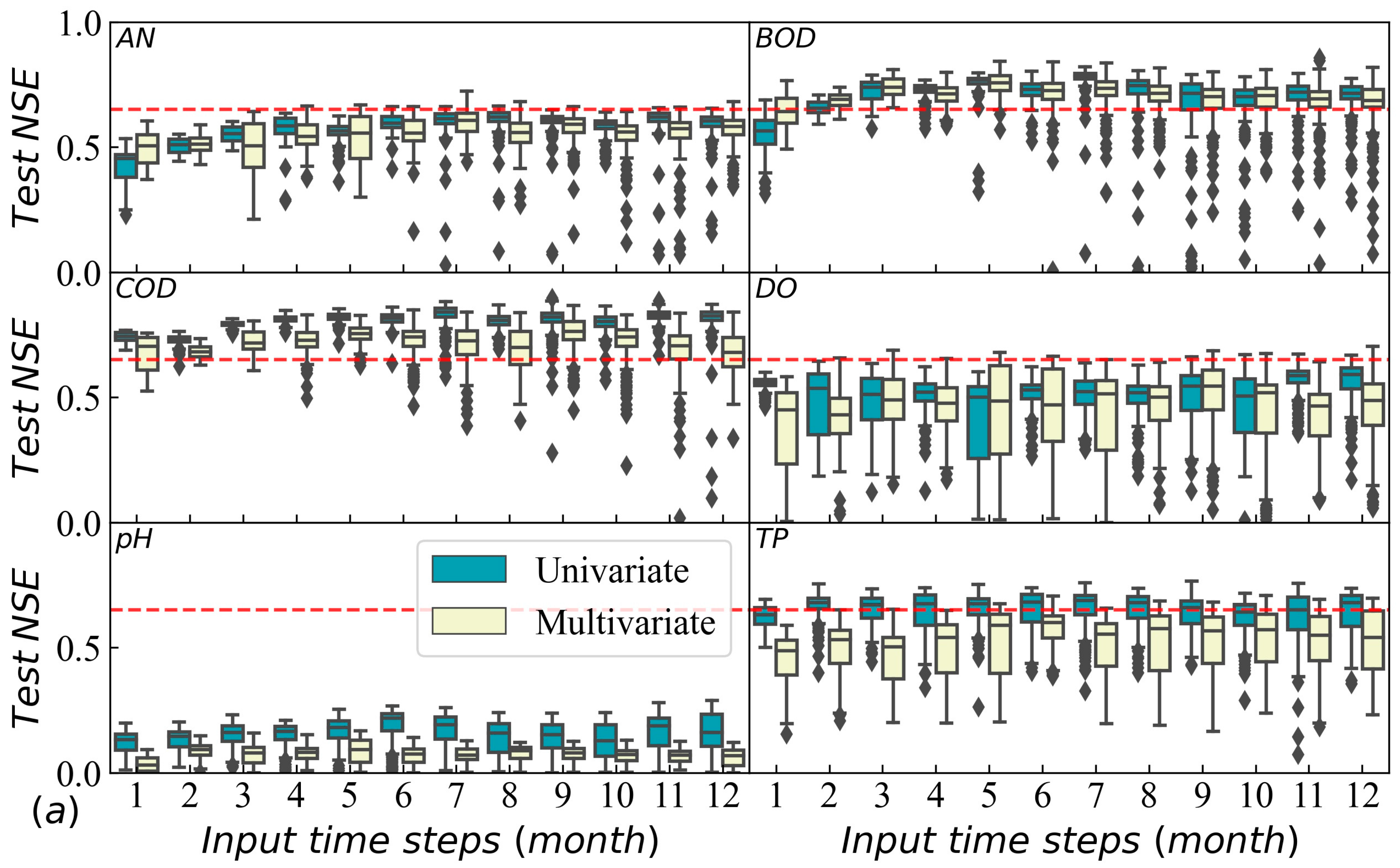
3.1. Model Accuracy Evaluation of Water Quality Prediction with Different Indexes

The accuracy of the model for various water quality indicators across different basins was examined and compared, considering the input variables and their respective lag times, as illustrated in Figure 4 and Figure 5.

For models with different input conditions (shown in Figure 4), when inputting more variables, most of the median NSEs of the YRB decreased by nearly 0.25 (Figure 4b), while, except for the pH, there was little deterioration in the performances of the models of the HRB (Figure 4a). However, LSTM models to predict the DO in the HRB performed better after inputting data for more water quality indicators (Figure 4a). Moreover, with more time-step data inputs, most LSTM models improved to some extent. Models for predicting the AN and TP of the YRB with multivariate inputs improved significantly when inputting more time-step data.

Figure 5 shows the differences in the performance of LSTM in the HRB and in the YRB under different inputs conditions. In the univariate input condition, LSTM models for the pH in the YRB are better than those for the pH in the HRB, while little difference between the YRB and HRB for predicting the DO or TP was found; the performances for predicting the AN, BOD, and COD in the HRB are much better than those for the YRB. As for the multivariate input condition, LSTM models for all water quality indicators of the HRB perform significantly better than those for the YRB. Nevertheless, the prediction accuracy gap between the HRB and YRB for the AN or TP was narrowed with increasing input time steps.

Table 2. Average ($\overline{X}$) and standard deviation ($\sigma$) of Nash–Sutcliffe Efficiency (NSE) values with the LSTM model.

Index	YRB		HRB		HSB
	$\overline{\mathit{X}}$	$\mathit{\sigma }$	$\overline{\mathit{X}}$	$\mathit{\sigma }$	$\overline{\mathit{X}}$	$\mathit{\sigma }$
BOD	0.060	0.038	0.773	0.070	0.523	0.167
COD	0.041	0.047	0.785	0.047	0.420	0.166
DO	0.375	0.174	0.623	0.055	0.074	0.110
NH3-N	0.233	0.038	0.631	0.082	0.706	0.043
TP	0.463	0.033	0.644	0.056	0.478	0.048
Ph	0.382	0.108	0.471	0.092	0.421	0.103

presents the average Nash–Sutcliffe Efficiency (NSE) values of the LSTM model for five key water quality indicators across three different basins: the Yangtze River Basin (YRB), the Haihe River Basin (HRB), and the Huangshui River Basin (HSB).

This table provides a comprehensive comparison of the model’s performance in predicting these indicators within each basin, highlighting the variability in prediction accuracy across different regions and parameters. The NSE values in the Haihe River Basin (HRB) are generally higher than those in the Yangtze River Basin (YRB) and the Huangshui River Basin (HSB). For instance, the HRB achieves NSE values of 0.773 for BOD, 0.785 for COD, 0.623 for DO, 0.631 for NH₃-N, and 0.644 for TP, indicating relatively high prediction accuracy. In contrast, the YRB shows much lower NSE values, such as 0.060 for BOD, 0.041 for COD, and 0.375 for DO, suggesting that the LSTM model performs less effectively in this basin. The HSB has intermediate NSE values, with 0.523 for BOD, 0.420 for COD, and 0.540 for DO. Notably, the HRB has the highest NSE for NH₃-N (0.631) and TP (0.644), while the YRB has the lowest NSE for most indicators, except for TP, where the HSB has the lowest value (0.478). The significant differences in NSE values across the three basins highlight the importance of considering regional characteristics when applying the LSTM model for water quality prediction. The higher NSE values in the HRB suggest that the model may be more suitable for this region due to specific environmental conditions or data quality. Conversely, the lower NSE values in the YRB indicate potential limitations of the model in this basin, possibly due to more complex hydrological processes or higher data variability. These findings emphasize the need for further investigation into the factors influencing model performance and the importance of tailoring model applications to specific basin conditions. Overall, while the LSTM model shows promise in some regions, its applicability and reliability vary significantly, necessitating careful evaluation and adaptation for different environments.

3.2. Confidence Analysis of LSTM for Water Quality Prediction in the Three Basins

We calculated the mean and standard deviation of the Nash–Sutcliffe Efficiency (NSE) for the predictions of BOD, COD, DO, NH₃-N, TP, and pH across all models in three watersheds. Based on these values, we determined the 95% confidence intervals. Subsequently, we obtained the widths of these confidence intervals under different confidence levels. The results are presented in

Table 3. Confidence interval (C_i) and confidence width $d_Z$ of three basins under confidence level of 95%.

Index	YRB		HSB		HRB
	Ci	${\mathit{d}}_{\mathit{Z}}$	Ci	${\mathit{d}}_{\mathit{Z}}$	Ci	${\mathit{d}}_{\mathit{Z}}$
BOD	[0.058, 0.062]	0.071	[0.769, 0.777]	0.011	[0.514, 0.532]	0.035
COD	[0.038, 0.044]	0.123	[0.782, 0.788]	0.007	[0.411, 0.429]	0.043
DO	[0.365, 0.385]	0.053	[0.620, 0.626]	0.010	[0.068, 0.080]	0.156
NH3-N	[0.231, 0.235]	0.019	[0.626, 0.636]	0.015	[0.704, 0.708]	0.007
TP	[0.461, 0.465]	0.008	[0.641, 0.647]	0.010	[0.475, 0.481]	0.011
Ph	[0.376, 0.388]	0.033	[0.465, 0.477]	0.023	[0.415, 0.427]	0.028

.

For all water quality indicators, as the confidence level increases, the width of the confidence intervals gradually expands, indicating increased prediction uncertainty at higher confidence levels. As shown in the table, at a 95% confidence level, the HRB demonstrates high prediction certainty for multiple key indicators. Particularly for biochemical oxygen demand (BOD), chemical oxygen demand (COD), dissolved oxygen (DO), and pH, the HRB exhibits the narrowest confidence intervals, implying relatively more stable prediction results. In contrast, the YRB shows lower prediction certainty for BOD, COD, and DO, with wider confidence intervals, while the HSB has relatively lower certainty in predicting DO and ammonia nitrogen (NH₃-N). Analyzing the specific performance for different water quality indicators, the HRB performs best in terms of the BOD, COD, and DO, with high prediction certainty and narrow confidence intervals. For the prediction of NH₃-N, the HSB performs optimally, with the smallest confidence interval width. Regarding the prediction of total phosphorus (TP), the YRB also demonstrates relatively high certainty. Overall, the HRB exhibits the best prediction stability, surpassing that of the HSB and YRB. Further analysis of the mean NSE values and prediction reliability levels for the three watersheds is presented in the Figure 6.

From Figure 6a, it can be seen that in terms of model simulation accuracy, the HRB performs the best, followed by the HSB, with the YRB performing the worst. Further analysis of the simulation reliability grades of the LSTM model for different indicators in the three watersheds in Figure 6b reveals that in the YRB, except for TP, the simulation reliability of the other indicators is at grade L1, indicating poor simulation performance and suggesting that the LSTM model may not be suitable for water quality prediction in the YRB; whereas in the HRB, the simulation performance of BOD and COD reaches grade L4 (excellent), and the simulation reliability of indicators such as DO and NH₃-N is also at grade L3, indicating good simulation performance and suggesting that the LSTM model is highly suitable for water quality prediction in the HRB; as for the HSB, the simulation performance of NH₃-N is good, and the simulation performance of other indicators is acceptable, indicating that with certain optimizations, the LSTM model can also be used for water quality prediction in the HSB watershed, and the prediction results are basically reliable.

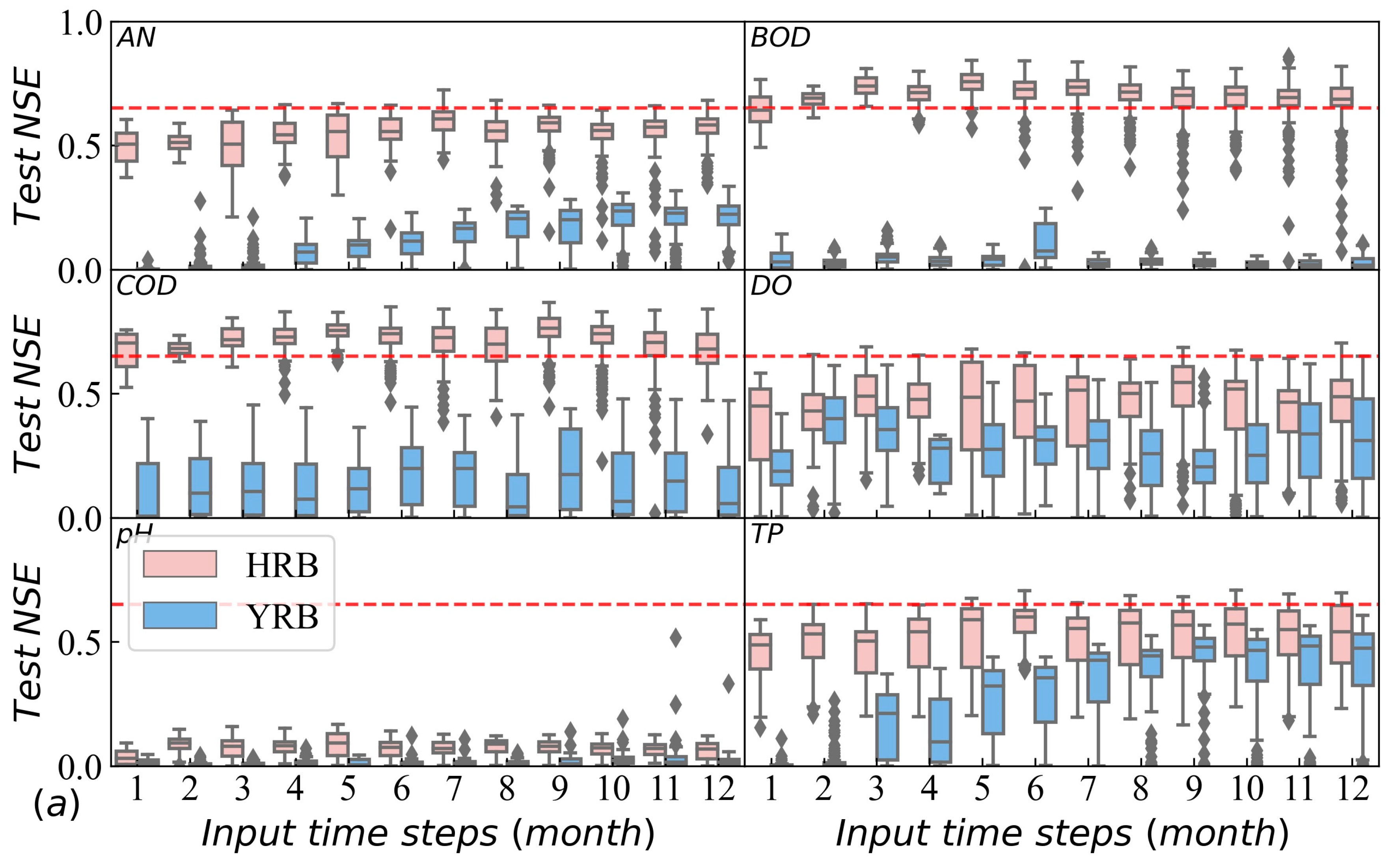
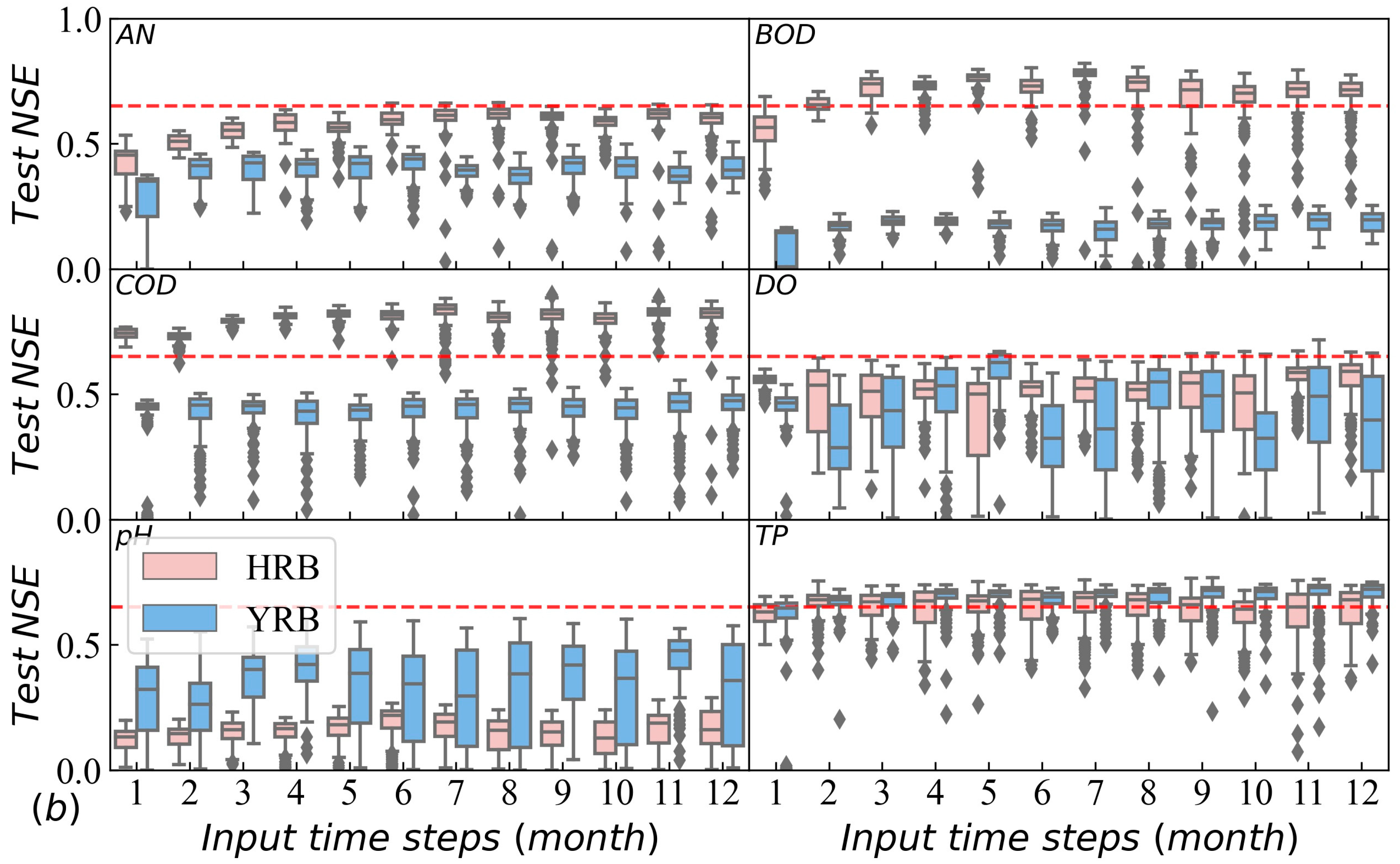
3.3. Influencing Factors of Model Performance in Different Basins

Most of these phenomena in Section 3.1 and Section 3.2 can be associated with temporal autocorrelation and cross-correlation coefficients, as mentioned in Section 2.2. For water quality indicators of the three basins, their autocorrelation coefficients are generally bigger than their cross-correlation coefficients with other indicators. In the YRB, the cross-correlation coefficients are much smaller (most MICs smaller than 0.2). As the volume of input data expanded in the LSTM model, water quality variables that exhibited low correlation with the output variables introduced significant amounts of redundant information. This influx of redundant data acted as a barrier, impeding the model’s capacity to discern meaningful and coherent patterns among the variables. Consequently, the prediction performance of the model suffered, as it struggled to differentiate between relevant and irrelevant information, leading to a decline in its overall accuracy and reliability [56,57,58]. Therefore, models with multivariate inputs of the YRB will be worse than those with univariate inputs of the YRB, which is consistent with the results. Similarly, TP has the biggest autocorrelation coefficients (MICs more than 0.6, 0.75, and 0.7 in the YRB, HRB, and HSB, respectively) among water quality indicators. However, except for the pH, water quality indicators in the HRB have bigger cross-correlation coefficients (MICs generally bigger than 0.5). In the YRB, LSTM performs the best in predicting the TP. And in the HRB, the prediction performance for the pH is the worst.

Therefore, the correlations between LSTM performances of water quality prediction and temporal autocorrelation/cross-correlation coefficients of water quality indicators warrant further exploration (as shown in Figure 7). In all scenarios, model performances are linearly dependent on the maximum values of temporal autocorrelation/cross-correlation coefficients. In addition, the linear relation is more stable and significant with the coefficients of determination for MICs ranging from 0.59 to 0.85. Different scenarios have almost the same slope in Figure 7. Significant variations are observed in the intercepts of the models, which can be attributed to various factors. One possible reason is the inherent differences across different basins, such as geographical characteristics, climate conditions, and water flow patterns. Another contributing factor could be the distinct input patterns used in the models, which may reflect variations in data collection methods, preprocessing steps, or the specific variables included in the analysis. These differences in intercepts highlight the complexity and variability inherent in modeling water quality across diverse basins and underscore the importance of considering basin-specific characteristics and input patterns when developing and applying such models.

Furthermore, pollutant concentrations of the HRB and HSB are much higher than those of the YRB (Table 1), which could be attributed to large geographical variations [1]. Additionally, the Haihe River Basin is a typical sluice-controlled river. The construction and operation of sluice dams change the flow and other hydrological factors of rivers, which have adverse effects on water [30]. The high pollutant concentration and poor fluidity of water in the HRB and HSB may be one of the reasons why water quality indicators in these two basins are more related than those in the YRB.

Thus, the relationship between concentration and variability of water quality indicators (described by the mean value and coefficient of variation (CV), respectively) and prediction performance (exhibited by the median NSE) has been investigated, as shown in Figure 8. The results revealed that little linear correlation exists between the mean concentration and prediction performance of water quality indicators with coefficients of determination (R²) as low as 0.10. Additionally, there is a certain correlation between model performances and CVs of water quality indicators with an R² of 0.44 and p-value < 0.05. Thus, the performance of the model demonstrates a pronounced and robust linear dependence on the maximum values of the temporal autocorrelation and cross-correlation coefficients of the water quality indicators. This suggests that the model’s predictive accuracy and reliability are significantly influenced by the strength and patterns of temporal relationships among the water quality indicators. Specifically, as the maximum values of these correlation coefficients increase, the model’s performance tends to improve, indicating that it is better able to capture and utilize the underlying temporal dynamics of the water quality data. This finding underscores the importance of considering temporal autocorrelation and cross-correlation in the development and optimization of water quality models.

In this study, forecasts for water quality in the YRB, a large, water-rich basin, were less accurate than those for the HRB and HSB, which are smaller, water-scarce basins. Considering that the HRB and HSB have smaller watershed areas and more intensive monitoring networks than the YRB, more data are available. The variation in water quality is small, which makes the autocorrelation and cross-correlation of water quality variables bigger. This makes the LSTM model more applicable in both basins. It also shows, from the other hand, that increasing the density of the water quality monitoring network and the amount of available water quality data for training can significantly improve the surface water quality prediction performances of the learning models [23].

4. Conclusions

In this study, we developed a comprehensive confidence evaluation method for assessing the performances of LSTM models in water quality prediction. This method was applied to three major river basins in China. By comparing the prediction performance of the LSTM model across these basins for various water quality indicators, including the AN, BOD, COD, DO, pH, and TP, we found that the LSTM model exhibited superior performance in the Haihe River Basin and the Huangshui River Basin. Specifically, the prediction accuracy was higher in these two basins, and the confidence intervals for water quality prediction were also wider, indicating greater reliability. Our analysis revealed that for indicators with higher temporal autocorrelation, such as TP and COD, the prediction accuracy was significantly higher. Further analysis revealed a linear association between the predictive accuracy of the LSTM model and the temporal autocorrelation as well as the inter-variable correlation coefficients of the water quality indicators. This finding underscores the importance of considering the specific data characteristics of the target indicators when applying LSTM models for water quality prediction. While the LSTM model is a powerful tool for time-series prediction, its application must be tailored to the specific characteristics of the basin and the data features of the target indicators. A thorough analysis of the data features and the underlying temporal relationships of the water quality indicators is essential to maximize the effectiveness of the LSTM model in different river basins.

References

1. Ahmed, A.N.; Othman, F.B.; Afan, H.A.; Ibrahim, R.K.; Fai, C.M.; Hossain, M.S.; Ehteram, M.; Elshafie, A. Machine learning methods for better water quality prediction. J. Hydrol. 2019, 578, 124084. [Google Scholar] [CrossRef]
2. Tung, T.M.; Yaseen, Z.M. A survey on river water quality modelling using artificial intelligence models: 2000–2020. J. Hydrol. 2020, 585, 124670. [Google Scholar] [CrossRef]
3. Kim, H.G.; Hong, S.; Jeong, K.-S.; Kim, D.-K.; Joo, G.-J. Determination of sensitive variables regardless of hydrological alteration in artificial neural network model of chlorophyll a: Case study of Nakdong River. Ecol. Model. 2019, 398, 67–76. [Google Scholar] [CrossRef]
4. Kim, S.E.; Seo, I.W. Artificial Neural Network ensemble modeling with conjunctive data clustering for water quality prediction in rivers. J. Hydro-Environ. Res. 2015, 9, 325–339. [Google Scholar] [CrossRef]
5. Ahmed, A.A.M.; Shah, S.M.A. Application of adaptive neuro-fuzzy inference system (ANFIS) to estimate the biochemical oxygen demand (BOD) of Surma River. J. King Saud Univ.-Eng. Sci. 2017, 29, 237–243. [Google Scholar] [CrossRef]
6. Mahmoodabadi, M.; Arshad, R.R. Long-term evaluation of water quality parameters of the Karoun River using a regression approach and the adaptive neuro-fuzzy inference system. Mar. Pollut. Bull. 2018, 126, 372–380. [Google Scholar] [CrossRef]
7. Yi, H.-S.; Park, S.; An, K.-G.; Kwak, K.-C. Algal Bloom Prediction Using Extreme Learning Machine Models at Artificial Weirs in the Nakdong River, Korea. Int. J. Environ. Res. Public Health 2018, 15, 2078. [Google Scholar] [CrossRef] [PubMed]
8. Fan, J.; Li, M.; Guo, F.; Yan, Z.; Zheng, X.; Zhang, Y.; Xu, Z.; Wu, F. Priorization of River Restoration by Coupling Soil and Water Assessment Tool (SWAT) and Support Vector Machine (SVM) Models in the Taizi River Basin, Northern China. Int. J. Environ. Res. Public Health 2018, 15, 2090. [Google Scholar] [CrossRef] [PubMed]
9. Ji, X.; Shang, X.; Dahlgren, R.A.; Zhang, M. Prediction of dissolved oxygen concentration in hypoxic river systems using support vector machine: A case study of Wen-Rui Tang River, China. Environ. Sci. Pollut. Res. 2017, 24, 16062–16076. [Google Scholar] [CrossRef]
10. Kratzert, F.; Klotz, D.; Brenner, C.; Schulz, K.; Herrnegger, M. Rainfall-runoff modelling using Long Short-Term Memory (LSTM) networks. Hydrol. Earth Syst. Sci. 2018, 22, 6005–6022. [Google Scholar] [CrossRef]
11. Antanasijević, D.; Pocajt, V.; Povrenović, D.; Perić-Grujić, A.; Ristić, M. Modelling of dissolved oxygen content using artificial neural networks: Danube River, North Serbia, case study. Environ. Sci. Pollut. Res. 2013, 20, 9006–9013. [Google Scholar] [CrossRef]
12. Li, L.; Jiang, P.; Xu, H.; Lin, G.; Guo, D.; Wu, H. Water quality prediction based on recurrent neural network and improved evidence theory: A case study of Qiantang River, China. Environ. Sci. Pollut. Res. 2019, 26, 19879–19896. [Google Scholar] [CrossRef]
13. Hochreiter, S.; Schmidhuber, J. Long Short-Term Memory. Neural Comput. 1997, 9, 1735–1780. [Google Scholar] [CrossRef]
14. Zhou, J.; Wang, Y.; Xiao, F.; Wang, Y.; Sun, L. Water Quality Prediction Method Based on IGRA and LSTM. Water 2018, 10, 1148. [Google Scholar] [CrossRef]
15. Barzegar, R.; Aalami, M.T.; Adamowski, J. Short-term water quality variable prediction using a hybrid CNN-LSTM deep learning model. Stoch. Environ. Res. Risk Assess. 2020, 34, 415–433. [Google Scholar] [CrossRef]
16. Liang, Z.; Zou, R.; Chen, X.; Ren, T.; Su, H.; Liu, Y. Simulate the forecast capacity of a complicated water quality model using the long short-term memory approach. J. Hydrol. 2020, 581, 124432. [Google Scholar] [CrossRef]
17. Liu, P.; Wang, J.; Sangaiah, A.; Xie, Y.; Yin, X. Analysis and Prediction of Water Quality Using LSTM Deep Neural Networks in IoT Environment. Sustainability 2019, 11, 2058. [Google Scholar] [CrossRef]
18. Song, C.; Yao, L.; Hua, C.; Ni, Q. A novel hybrid model for water quality prediction based on synchro squeezed wavelet transform technique and improved long short-term memory. J. Hydrol. 2021, 603, 126879. [Google Scholar] [CrossRef]
19. Luo, Q.; Peng, D.; Shang, W. Water quality analysis based on LSTM and BP optimization with a transfer learning model. Environ. Sci. Pollut. Res. 2023, 30, 124341–124352. [Google Scholar] [CrossRef]
20. Zou, Q.; Xiong, Q.; Li, Q.; Yi, H.; Yu, Y.; Wu, C. A water quality prediction method based on the multi-time scale bidirectional long short-term memory network. Environ. Sci. Pollut. Res. 2020, 27, 16853–16864. [Google Scholar] [CrossRef]
21. Ueda, F.; Tanouchi, H.; Egusa, N.; Yoshihiro, T. A Transfer Learning Approach Based on Radar Rainfall for River Water-Level Prediction. Water 2024, 16, 607. [Google Scholar] [CrossRef]
22. Chang, F.-J.; Tsai, Y.-H.; Chen, P.-A.; Coynel, A.; Vachaud, G. Modeling water quality in an urban river using hydrological factors—Data driven approaches. J. Environ. Manag. 2015, 151, 87–96. [Google Scholar] [CrossRef]
23. Chen, K.; Chen, H.; Zhou, C.; Huang, Y.; Qi, X.; Shen, R.; Liu, F.; Zuo, M.; Zou, X.; Wang, J.; et al. Comparative analysis of surface water quality prediction performance and identification of key water parameters using different machine learning models based on big data. Water Res. 2020, 171, 115454. [Google Scholar] [CrossRef]
24. Nemati, S.; Fazelifard, M.H.; Terzi, Ö.; Ghorbani, M.A. Estimation of dissolved oxygen using data-driven techniques in the Tai Po River, Hong Kong. Environ. Earth Sci. 2015, 74, 4065–4073. [Google Scholar] [CrossRef]
25. Parmar, K.S.; Makkhan, S.J.S.; Kaushal, S. Neuro-fuzzy-wavelet hybrid approach to estimate the future trends of river water quality. Neural Comput. Appl. 2019, 31, 8463–8473. [Google Scholar] [CrossRef]
26. Wang, C.; Shan, B.; Zhang, H.; Zhao, Y. Limitation of spatial distribution of ammonia-oxidizing microorganisms in the Haihe River, China, by heavy metals. J. Environ. Sci. 2014, 26, 502–511. [Google Scholar] [CrossRef]
27. Zhu, S.; Luo, X.; Yuan, X.; Xu, Z. An improved long short-term memory network for streamflow forecasting in the upper Yangtze River. Stoch. Environ. Res. Risk Assess. 2020, 34, 1313–1329. [Google Scholar] [CrossRef]
28. Zhu, Y.; Drake, S.; Lü, H.; Xia, J. Analysis of temporal and spatial differences in eco-environmental carrying capacity related to water in the Haihe river basins, China. Water Resour. Manag. 2010, 24, 1089–1105. [Google Scholar] [CrossRef]
29. Xu, J.; Liu, R.; Ni, M.; Zhang, J.; Ji, Q.; Xiao, Z. Seasonal variations of water quality response to land use metrics at multi-spatial scales in the Yangtze River basin. Environ. Sci. Pollut. Res. 2021, 28, 37172–37181. [Google Scholar] [CrossRef]
30. Wang, Y.; Ding, X.; Chen, Y.; Zeng, W.; Zhao, Y. Pollution source identification and abatement for water quality sections in Huangshui River basin, China. J. Environ. Manag. 2023, 344, 118326. [Google Scholar] [CrossRef]
31. Maguire, J.; Cusack, C.; Ruiz-Villarreal, M.; Silke, J.; McElligott, D.; Davidson, K. Applied simulations and integrated modelling for the understanding of toxic and harmful algal blooms (ASIMUTH): Integrated HAB forecast systems for Europe’s Atlantic Arc. Harmful Algae 2016, 53, 160–166. [Google Scholar] [CrossRef] [PubMed]
32. Salacinska, K.; El Serafy, G.Y.; Los, F.J.; Blauw, A. Sensitivity analysis of the two dimensional application of the Generic Ecological Model (GEM) to algal bloom prediction in the North Sea. Ecol. Model. 2010, 221, 178–190. [Google Scholar] [CrossRef]
33. Li, R. Water quality forecasting of Haihe River based on improved fuzzy time series model. Desalination Water Treat. 2018, 106, 285–291. [Google Scholar] [CrossRef]
34. Liang, N.; Zou, Z.; Wei, Y. Regression models (SVR, EMD and FastICA) in forecasting water quality of the Haihe River of China. Desalination Water Treat. 2019, 154, 147–159. [Google Scholar] [CrossRef]
35. Liu, X.B.; Peng, W.Q.; He, G.J.; Liu, J.L.; Wang, Y.C. A Coupled Model of Hydrodynamics and Water Quality for Yuqiao Reservoir in Haihe River Basin. J. Hydrodyn. 2008, 20, 574–582. [Google Scholar] [CrossRef]
36. Zhang, L.; Zou, Z.H.; Zhao, Y.F. Application of chaotic prediction model based on wavelet transform on water quality prediction. IOP Conf. Ser. Earth Environ. Sci. 2016, 39, 012001. [Google Scholar] [CrossRef]
37. Zhang, X.; Jiang, H.L.; Zhang, Y.Z. The Hybrid Method to Predict Biochemical Oxygen Demand of Haihe River in China. Adv. Mater. Res. 2012, 610–613, 1066–1069. [Google Scholar] [CrossRef]
38. Chen, S.; Fang, G.; Huang, X.; Zhang, Y. Water Quality Prediction Model of a Water Diversion Project Based on the Improved Artificial Bee Colony–Backpropagation Neural Network. Water 2018, 10, 806. [Google Scholar] [CrossRef]
39. Deng, W.; Wang, G.; Zhang, X. A novel hybrid water quality time series prediction method based on cloud model and fuzzy forecasting. Chemom. Intell. Lab. Syst. 2015, 149, 39–49. [Google Scholar] [CrossRef]
40. Di, Z.; Chang, M.; Guo, P. Water Quality Evaluation of the Yangtze River in China Using Machine Learning Techniques and Data Monitoring on Different Time Scales. Water 2019, 11, 339. [Google Scholar] [CrossRef]
41. Zhou, C.; Gao, L.; Gao, H.; Peng, C. Pattern Classification and Prediction of Water Quality by Neural Network with Particle Swarm Optimization. In Proceedings of the 2006 6th World Congress on Intelligent Control and Automation, Dalian, China, 21–23 June 2006; pp. 2864–2868. [Google Scholar] [CrossRef]
42. Gao, Y.; Zhang, W.; Li, Y.; Wu, H.; Yang, N.; Hui, C. Dams shift microbial community assembly and imprint nitrogen transformation along the Yangtze River. Water Res. 2021, 189, 116579. [Google Scholar] [CrossRef] [PubMed]
43. Hu, M.; Liu, Y.; Zhang, Y.; Shen, H.; Yao, M.; Dahlgren, R.A.; Chen, D. Long-term (1980–2015) changes in net anthropogenic phosphorus inputs and riverine phosphorus export in the Yangtze River basin. Water Res. 2020, 177, 115779. [Google Scholar] [CrossRef]
44. Liu, X.; Beusen, A.H.W.; Van Beek, L.P.H.; Mogollón, J.M.; Ran, X.; Bouwman, A.F. Exploring spatiotemporal changes of the Yangtze River (Changjiang) nitrogen and phosphorus sources, retention and export to the East China Sea and Yellow Sea. Water Res. 2018, 142, 246–255. [Google Scholar] [CrossRef] [PubMed]
45. Dang, B.; Mao, D.; Xu, Y.; Luo, Y. Conjugative multi-resistant plasmids in Haihe River and their impacts on the abundance and spatial distribution of antibiotic resistance genes. Water Res. 2017, 111, 81–91. [Google Scholar] [CrossRef]
46. Bao, Z.; Zhang, J.; Wang, G.; Fu, G.; He, R.; Yan, X.; Jin, J.; Liu, Y.; Zhang, A. Attribution for decreasing streamflow of the Haihe River basin, northern China: Climate variability or human activities? J. Hydrol. 2012, 460–461, 117–129. [Google Scholar] [CrossRef]
47. Zheng, M.; Zheng, H.; Wu, Y.; Xiao, Y.; Du, Y.; Xu, W.; Lu, F.; Wang, X.; Ouyang, Z. Changes in nitrogen budget and potential risk to the environment over 20 years (1990–2010) in the agroecosystems of the Haihe Basin, China. J. Environ. Sci. 2015, 28, 195–202. [Google Scholar] [CrossRef] [PubMed]
48. Reshef, D.N.; Reshef, Y.A.; Finucane, H.K.; Grossman, S.R.; McVean, G.; Turnbaugh, P.J.; Lander, E.S.; Mitzenmacher, M.; Sabeti, P.C. Detecting novel associations in large data sets. Science 2011, 334, 1518–1524. [Google Scholar] [CrossRef] [PubMed]
49. Zhang, J.; Zhu, Y.; Zhang, X.; Ye, M.; Yang, J. Developing a Long Short-Term Memory (LSTM) based model for predicting water table depth in agricultural areas. J. Hydrol. 2018, 561, 918–929. [Google Scholar] [CrossRef]
50. Panfeng, B.; Songlin, Z.; Hongyu, C.; Caiwei, L.; Pengtao, W.; Lichang, Q. Structural monitoring data repair based on a long short-term memory neural network. Sci. Rep. 2024, 14, 9974. [Google Scholar] [CrossRef]
51. Bennett, N.D.; Croke, B.F.W.; Guariso, G.; Guillaume, J.H.A.; Hamilton, S.H.; Jakeman, A.J.; Marsili-Libelli, S.; Newham, L.T.H.; Norton, J.P.; Perrin, C.; et al. Characterising performance of environmental models. Environ. Model. Softw. 2013, 40, 1–20. [Google Scholar] [CrossRef]
52. Sadiki, N.; Jang, D.W. Estimation of Hydraulic and Water Quality Parameters Using Long Short-Term Memory in Water Distribution Systems. Water 2024, 16, 3028. [Google Scholar] [CrossRef]
53. Gachloo, M.; Liu, Q.; Song, Y.; Wang, G.; Zhang, S.; Hall, N. Using Machine Learning Models for Short-Term Prediction of Dissolved Oxygen in a Microtidal Estuary. Water 2024, 16, 1998. [Google Scholar] [CrossRef]
54. Ritter, A.; Muñoz-Carpena, R. Performance evaluation of hydrological models: Statistical significance for reducing subjectivity in goodness-of-fit assessments. J. Hydrol. 2013, 480, 33–45. [Google Scholar] [CrossRef]
55. Moriasi, D.N.; Arnold, J.G.; Van Liew, M.W.; Bingner, R.L.; Harmel, R.D.; Veith, T.L. Model evaluation guidelines for systematic quantification of accuracy in watershed simulations. Trans. ASABE 2007, 50, 885–900. [Google Scholar] [CrossRef]
56. Galelli, S.; Humphrey, G.B.; Maier, H.R.; Castelletti, A.; Dandy, G.C.; Gibbs, M.S. An evaluation framework for input variable selection algorithms for environmental data-driven models. Environ. Model. Softw. 2014, 62, 33–51. [Google Scholar] [CrossRef]
57. Maier, H.R.; Jain, A.; Dandy, G.C.; Sudheer, K.P. Methods used for the development of neural networks for the prediction of water resource variables in river systems: Current status and future directions. Environ. Model. Softw. 2010, 25, 891–909. [Google Scholar] [CrossRef]
58. Maier, H.R.; Dandy, G.C. Neural networks for the prediction and forecasting of water resources variables: A review of modelling issues and applications. Environ. Model. Softw. 2000, 15, 101–124. [Google Scholar] [CrossRef]
Figure 1. Geographical regions and placement of water quality stations.
Water 17 01050 g001
Figure 2. Temporal autocorrelation and cross-correlation coefficients based on Maximal Information Coefficient (MIC) of each water quality indicator in the same basin with a lag time from 1 to 12 months. The abbreviations mean: biochemical oxygen demand (BOD), chemical oxygen demand (COD), dissolved oxygen (DO), ammonia nitrogen (AN), total phosphorus (TP), and hydrogen ion concentration (pH), the Huangshui River Basin (HSB), the Haihe River Basin (HRB), and the Yangtze River Basin (YRB). Figure (af) mean temporal autocorrelation and cross-correlation coefficients of AN, BOD, CODMN, DO, PH and TP, respectively.
Water 17 01050 g002
Figure 3. Conceptual illustration of memory block in LSTM.
Water 17 01050 g003
Figure 4. Comparison of distribution of NSE values for water quality indicators of (a) the HRB and (b) YRB predicted using different input conditions. The red dotted lines represent the threshold of acceptable model performance (NSE = 0.65).
Water 17 01050 g004aWater 17 01050 g004b
Figure 5. A comparison of the distribution of NSE values for each water quality indicator across different basins, predicted using (a) univariate inputs and (b) multivariate inputs. The red dashed lines indicate the threshold for acceptable model performance (NSE = 0.65).
Water 17 01050 g005aWater 17 01050 g005b
Figure 6. Simulation reliability grades of LSTM model for different indicators in three watersheds. (a) Mean NSE; (b) confidence levels.
Water 17 01050 g006
Figure 7. Scatter plots illustrating the relationship between model performance and input–output correlations, as calculated using the MIC, are presented for the following cases: (a) the YRB with multivariate inputs, (b) the YRB with univariate inputs, (c) the HRB with multivariate inputs, and (d) the HRB with univariate inputs. In these plots, R2 represents the coefficient of determination, while p denotes the p-value from the statistical significance test of linear regression.
Water 17 01050 g007
Figure 8. Scatter plot demonstration of the relationship between (a) the mean concentration and (b) coefficient of variation of water quality indicators and prediction performance.
Water 17 01050 g008