Simulation of Tidal Oscillations in the Pará River Estuary Using the MOHID-Land Hydrological Model

Abstract

Recent studies have incorporated tidal elevation into hydrological models, yet they have not focused on simulating or evaluating tidal processes within these frameworks. Integrating tidal dynamics improves the representation of terrestrial–coastal interactions, including groundwater fluctuations, vegetation dynamics, and sediment transport. This study evaluates the capability of MOHID-Land, a physically based hydrological model, to simulate macro-tidal conditions in an Amazonian estuary. MOHID-Land enables tidal simulation by incorporating water-level time series as boundary conditions. A sensitivity analysis was conducted to (i) evaluate two global tidal models as boundary conditions; (ii) verify the impact of hydrological processes on water levels; and (iii) assess the effect of different bathymetries on water dynamics. The model effectively simulated tidal oscillations with good accuracy across eight tidal stations, although the inner stations required improved bathymetry. The Reference, Atmosphere, Porous Media and Vegetation (AtPmVg), and Finite Element Solution (FES) version 2014 (FES2014) simulations yielded similar water levels and goodness-of-fit metrics. While MOHID-Land is robust, and water level modeling is insensitive to meteorological, soil, or vegetation parameters, the model is highly sensitive to bathymetry. This study enhances the understanding of the applicability of hydrological models in terrestrial–coastal modeling.

1. Introduction

Inland and coastal water bodies are crucial to the global biosphere [1]. These systems are interconnected through the exchange of water, nutrients, sediments, and pollutants, creating a dynamic system with components that can impact one another. However, coastal areas are under constant pressure as they are increasingly altered by human activities [2] and land reclamation [3], as well as by climate drivers such as sea level rise [4]. These pressures can modify the coastal dynamics, leading to consequences such as salinity intrusion into aquifers [5], the reduced availability of potable water [6], soil biogeochemical modifications, and shifts in vegetation types and diversity [7].

Accurate modeling of the physical, chemical, and biological processes of those systems is important for the effective management of water resources, natural hazards, sediment dynamics, navigation, and agriculture [8,9]. Hydrological models and hydrodynamic models have traditionally been developed independently, each focusing on specific components of the water system. Hydrological models, typically used on inland water bodies, rely on simplified assumptions of natural systems [10,11] to address the water cycle and its hydrological processes [12], such as precipitation, infiltration, surface runoff, and groundwater flow. They can be classified as empirical, conceptual, or physically based. Conversely, hydrodynamic models simulate water movement, waves, and sediment transport in oceans and coastal zones, relying on physical governing equations [13], consequently being described as physically based models. However, these models tend to overlook terrestrial hydrological processes, such as evapotranspiration and soil infiltration, which are important to overall environmental water balance. To address these limitations, coupled hydrological–hydrodynamic models have been developed [14].

However, there are recent efforts to integrate tidal elevation into hydrological models. For example, Mansanarez et al. [15] adapted the Génie Rural (GR) semi-distributed rainfall-runoff model (GRSD model) [16] to consider tidal influences in the river mouth area. This approach improved the interpretation of tidal-affected locations, simulating the delay of the streamflow caused by tidal influence. Zhang et al. [17] adapted the Penn State integrated hydrological model (PIHM; [18]) to develop the PIHM-Wetland, a regional scale, spatially distributed, and physically based model. Originally, PIHM was a hydrological model that simulates a single watershed, while PIHM-Wetland is designed as a regional-scale model, integrating coastal processes such as tides, sea-level rise, and saltwater intrusion, and considers the effects of inundation on coastal wetland hydrology.

Despite these advancements, there are still improvements to be made in integrating tidal dynamics into hydrological models. Mansanarez et al. [15] worked with a lumped model based on empirical equations, which limited its ability to accurately represent spatial variations and detailed tidal effects. In contrast, Zhang et al. [17] used a physically based model that was calibrated for evapotranspiration and groundwater levels. However, neither group explores nor simulates tidal dynamics in hydrological models. This research aims to evaluate the capability of a hydrological model to simulate macro-tidal conditions in an Amazonian estuary, contributing new insights to the integration of tidal processes and enhancing the representation of coastal wetland hydrology.

The MOHID-Land model was used in this study, which is a physically based hydrological model that employs a fully distributed approach, solving the full Saint-Venant equations on a 2D horizontal grid [19]. MOHID-Land simulates vegetation and soil processes, which influence how precipitation is stored and managed in the system. Vegetation plays a crucial role in the process through evapotranspiration, which includes transpiration, interception loss, and bare soil evaporation [20]. Additionally, once precipitation reaches the ground, soil dynamics are important: the soil absorbs and stores water based on certain properties, such as texture, moisture levels [21], and organic content [22].

The MOHID-Land model incorporates water level time series as boundary conditions, allowing for the simulation of tidal oscillations. These boundary conditions can be derived from tide gauge data, satellite altimetry, regional or local hydrodynamic models, or global tidal models. In this study, global tidal models were used due to their ability to provide continuous spatial coverage and predict tidal variations across large domains, including areas where in situ measurements are unavailable.

However, global tidal models typically perform better in open ocean conditions than in coastal areas [23], due to the nonlinear effects from shallow water, complex bathymetry, friction, and local resonance [23,24]. These factors reduce the model accuracy near the coast. Assessing the performance of two global tidal models is essential to determine their suitability for representing tidal dynamics accurately in the Pará River estuary.

A sensitivity analysis was conducted to (i) evaluate the influence of two global tidal models as boundary conditions; (ii) verify the impact of hydrological processes on water levels; and (iii) assess the effects of different bathymetries on water dynamics.

Integrating tidal dynamics into hydrological models like MOHID-Land enhances their representation and understanding of terrestrial–coastal interactions. Tidal fluctuations influence various environmental factors, including groundwater fluctuations (referred to as the tidal effect) [5], vegetation establishment and development [25], and sedimentological processes [26]. By incorporating tidal dynamics, MOHID-Land provides a more comprehensive understanding of the intricate interactions within estuarine and coastal systems. Additionally, this research lays the groundwork for future studies focused on estuarine wetlands, emphasizing the influence of tidal simulations on vegetation dynamics, evapotranspiration, and groundwater availability.

2. Materials and Methods

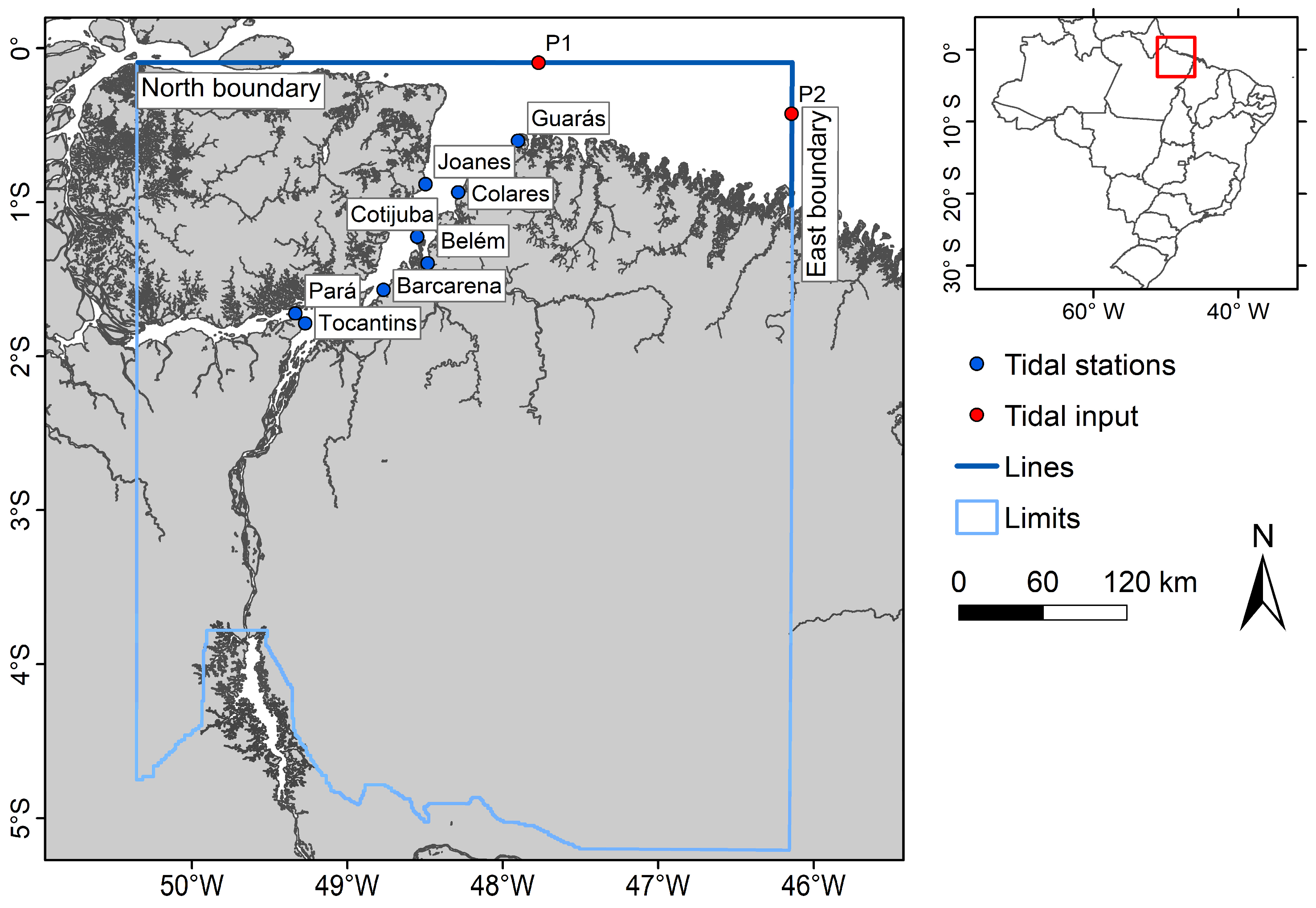
2.1. Study Area

The study area is within the Pará River estuary, located in the Tocantins-Araguaia watershed, Pará, Brazil. Figure 1 shows the study area location, along with its boundaries, grid limits, and the eight tidal stations used in calibration.

The climate comprises two distinct seasons: the rainy season (summer), between December and May, with peaks of rainfall typically occurring from February to April; and the dry season (winter), which extends from June to November, with September and October being the driest months [27].

The estuary has variable dimension, from 1 km upstream to, approximately, 50 km downstream [28]. The estuary drains directly into the Atlantic Ocean. The total annual average discharge (residual transport) ranges from 13,600 m³·s⁻¹ [29] to 21,000 m³·s⁻¹ [30]. The Pará River estuary receives a water contribution from the Tocantins-Araguaia watershed, mainly in the rainy season, and from the Amazon River via the Breves strait in the dry season [30,31,32]. Other important tributaries are found in the right margins of the estuary, such as Guamá, Acará, and the Moju River [28].

The estuary is semidiurnal, with a meso- to macro-tidal pattern, where tidal heights reach approximately 4 m in the main channel [32]. In the main channel, as the tidal wave moves upstream, it is attenuated, and the tidal amplitude decreases. Tides can be decomposed into harmonic components, which are periodic oscillations driven by gravitational forces from the Moon and the Sun. Each harmonic has its own frequency, amplitude, and phase. In the Pará River estuary, the combined amplitudes of the M₂, S₂, O₁, and K₁ components contribute approximately 60% of the total tidal energy, with M₂ as the primary energy source [32,33].

2.2. Hydrological Model

The MOHID-Land model was implemented in the study area to simulate water levels in the Pará River estuary. MOHID-Land is a component of the MOHID water modeling system, a physically based model that is spatially distributed, with variable time steps. It is used to model the water cycle in inland water bodies [34], at watershed scale [35], in reservoirs [36], or at the plot and field scale [37]. MOHID-Land simulates the water cycle across four main compartments: atmosphere, porous media, soil surface, and river network [35]. While the atmosphere is not explicitly simulated, it provides surface boundary conditions. Water movement between compartments follows mass and momentum conservation equations, using a finite volume approach.

Surface runoff is modeled using the 2D full Saint-Venant equation in conservative form, considering advection, pressure, and friction forces [35]. Porous media flow is solved considering a 3D domain, with variable vertical layers, in which infiltration is estimated according to Darcy’s law, and the infiltrated water moves according to the Richards equation [35,37]. Soil hydraulic properties are defined by the van Genuchten–Mualem functional relationships [35,37,38,39].

Reference evapotranspiration rates (ET_o, LT⁻¹) are calculated using the FAO Penman–Monteith equation [40]. The crop evapotranspiration rate (ET_c, LT⁻¹) is the product of ET_o and a single crop coefficient (K_c). The (K_c) of each vegetation type is imposed within the model, assuming a constant value for the entire growing season or a crop stage-dependent value, as used by Allen et al. [40]. ET_c values are partitioned into potential soil evaporation (E_p, L·T⁻¹) and crop transpiration (T_p) as a function of the leaf area index (LAI, L²·L⁻²), following the model developed by Ritchie [41].

An important feature of MOHID-Land is its modular structure, which is divided into components that handle both water quantity and quality. The quantity-related modules include Atmosphere, Runoff, Porous Media, Vegetation, Drainage Network, Irrigation, and Reservoirs. The quality-related modules consist of Porous Media Properties and Runoff Properties. Each module can be independently activated or deactivated, except for the Runoff module, which remains essential to the model’s operation. Only quantity-related modules were used in the scenarios, such as the Atmosphere, Runoff, Porous Media, and Vegetation modules.

2.3. Model Implementation

The model was implemented using a uniform grid with a resolution of 1 × 1 km, and four different scenarios were considered. Two tidal models were chosen as tidal input, namely, the TOPEX/POSEIDON tidal model (TPXO), specifically the Regional Amazon Shelf 1/60° model [42], hereafter named TPXO, and Finite Element Solution (FES) version 2014, described hereafter as FES2014. FES2014 was developed by LEGOS, NOVELTIS, and Collecte Localisation Satellites (CLS), and distributed by Aviso with support from the Centre National d’Etudes Spatiales (CNES) (http://www.aviso.altimetry.fr, accessed on 21 March 2024).

The TPXO model group was chosen due to previous applications in the study area [43,44], while the FES2014 model was chosen because it has been previously applied in many hydrodynamic models implemented using MOHID-Water [45,46]. Data from both models were extracted for two points, with P1 and P2 representing the tidal elevations in the North and East boundaries, respectively (Figure 1).

The Reference scenario focused solely on free surface flow, with only the Runoff module activated, and the TPXO was used as the tidal input. The Atmosphere, Porous Media, and Vegetation (AtPmVg) scenario incorporated atmospheric forcing factors such as precipitation, air temperature, wind velocity, solar radiation, cloud cover, and relative humidity, along with infiltration, exfiltration, bare soil evaporation, plant development, interception loss, and evapotranspiration. Alongside the Runoff module, the Atmosphere, Porous Media, and Vegetation modules were activated.

In the FES2014 scenario, TPXO boundary conditions were replaced with the FES2014 model. Lastly, the Bathymetry scenario considered the replacement of the bathymetry in the Reference scenario with data from the Brazilian Sea Observatory [47]. Both scenarios kept the same configuration as that used in the Reference scenarios, using only the Runoff module. All scenarios had the same river inputs.

The simulations were conducted from 1 November 2012 to 1 January 2013, with the initial eight days designated as the warm-up period. Table 1 details the general inputs used in the simulations.

Topographic and bathymetric data were merged to create a digital terrain model (DTM) for the study area. Topography data were sourced from United States Geological Survey (USGS) raster images [48] and from GTOPO30, with a resolution of 1 × 1 km, which was interpolated into the simulation grid. As the model grid was coarser, there was no need for a high-resolution dataset. Bathymetry data were sourced from two different databases to implement different scenarios, the Reference and Bathymetry simulations (Figure 2).

The Reference bathymetry dataset was developed by the Research Laboratory for Marine Environmental Monitoring (Laboratório de Pesquisa em Monitoramento Ambiental Marinho—LAPMAR), using in situ data and bathymetry data from the nautical charts of the Brazilian Navy (Marinha do Brasil) [49]. This bathymetry dataset was interpolated to the simulation grid using the inverse distance weighted (IDW) method and was later merged with the data from the topography to create the DTM (Figure 3a). The bathymetry was then smoothed to remove the sandbanks from the estuary mouth because, during calibration, the banks deformed the tidal wave. Reference bathymetry was used in the Reference, AtPmVg, and FES2014 simulations.

Table 1. Input data and the sources applied to the Pará River estuary model.

Input Data	Scenario	Sources
Digital Elevation	All	USGS—GTOPO30 [48]
Roughness	All	Copernicus land-use maps [50]
Bathymetry	Reference, AtPmVg, FES2014	LAPMAR bathymetry, with banks removed and smoothed
	Bathymetry	Brazilian Sea Observatory [47]
Vegetation and Land-Use	All	Annual Mapping Project of Land Use and Coverage (MapBiomas) [51]
Soil	All	SOTER-based soil parameter estimates (SOTWIS) [52]
Atmosphere	All	National Water Agency/Agência Nacional das Águas [53]
Discharge	All	National Water Agency/Agência Nacional das Águas [53]
Tidal elevation	Reference, AtPmVg, Bathymetry	TOPEX/POSEIDON tidal model (TPXO), Regional Amazon Shelf 1/60° model version [42]
	FES2014	Finite Element Solution—FES2014

Table 1. Input data and the sources applied to the Pará River estuary model.

Input Data	Scenario	Sources
Digital Elevation	All	USGS—GTOPO30 [48]
Roughness	All	Copernicus land-use maps [50]
Bathymetry	Reference, AtPmVg, FES2014	LAPMAR bathymetry, with banks removed and smoothed
	Bathymetry	Brazilian Sea Observatory [47]
Vegetation and Land-Use	All	Annual Mapping Project of Land Use and Coverage (MapBiomas) [51]
Soil	All	SOTER-based soil parameter estimates (SOTWIS) [52]
Atmosphere	All	National Water Agency/Agência Nacional das Águas [53]
Discharge	All	National Water Agency/Agência Nacional das Águas [53]
Tidal elevation	Reference, AtPmVg, Bathymetry	TOPEX/POSEIDON tidal model (TPXO), Regional Amazon Shelf 1/60° model version [42]
	FES2014	Finite Element Solution—FES2014

The second bathymetry dataset, used only in the Bathymetry simulation, was developed by the Marine, Environment, and Technology Center (MARETEC) for earlier hydrodynamic research using the MOHID-Water model. This bathymetry, available online from the Brazilian Sea Observatory [47], is based on nautical charts implemented for a variable-spaced grid of 1/24 (~4.6 km) in the open ocean to 1/60 (~1.8 km) in the inner estuary. The bathymetry was extracted from the hydrodynamic model grid into an XYZ file and was subsequently interpolated into the MOHID-Land grid without further modifications (Figure 3b). This dataset is more realistic than that of the Reference bathymetry, which underwent further alterations.

Vegetation types in the study area were taken from land-cover maps developed by the Annual Mapping Project of Land Use and Coverage in Brazil [51] for the year 2010. A total of 10 vegetation types were identified, with the forest-evergreen type, primarily attributed to the Amazon rainforest, covering approximately 51% of the area. Pasture accounted for nearly 30%, while water bodies represented around 12%, and grasslands occupied 5%. Other land uses, such as orchards (perennial crops like citrus and coffee), range-brush (scrubland), wetlands, soybean crops, and areas without vegetation (urban areas and mining sites), collectively constitute less than 2% of the study area (Figure 3a).

The Manning coefficient on the land surface was derived from the Copernicus CORINE Land Cover maps [50]. Figure 3b shows the spatial distribution of the Manning coefficient values. CORINE Land Cover maps were used due to the simplification of the land cover classes.

Soil data were obtained using SOTER-based soil parameter estimates (SOTWIS) for Latin America and the Caribbean, covering five horizons from 0 to 1 m at 0.2 m intervals [52]. To manage the dataset, a simplified classification based on the United States Department of Agriculture (USDA) [54] textures was created, identifying 5 soil types for each horizon, for a total of 25 soils (Figure 3c). The soil textures found were clay (C), loamy sand (LS), sandy loam (SL), sand (S), loam (L), sandy clay loam (SCL), and silty clay loam (SiCL).

The total soil depth was defined as 5 m because MOHID-Land requires the soil depth to exceed the vegetation root depth for it to accurately simulate water uptake by plants, ensuring a realistic representation of the natural environment. Thus, soil depth was divided into five layers with a thickness of 0.2, 0.4, 0.6, 0.8, and 3 m, working from top to bottom. Soil hydraulic parameters were determined using the Rosetta model [55].

Meteorological data were sourced from the ERA5-Reanalysis dataset [56], including wind speed, dew point temperature, air temperature, surface solar radiation, and surface pressure. Precipitation data were collected from the National Water Agency of Brazil (ANA) [53], following the methodology presented by Pereira et al. [57].

Two major rivers contribute to the estuary, namely, the Tocantins-Araguaia River and the Amazon River, flowing through Breves Strait. Flow data for the Tocantins-Araguaia River was obtained from the Reservoir Monitoring System (SAR, in Portuguese) for the Tucuruí Reservoir [58]. The outflow data were used as a boundary condition in the model, spanning from 2008 to 2022.

To define the discharge from Breves Strait, the methodology described by Prestes et al. [30] was applied. Historical discharge data from three ANA monitoring stations representing the Amazon, Tapajós, and Xingu rivers was analyzed for the period from 2005 to 2022 (

Table 2. Details from the monitoring stations operated by ANA within the Amazon Basin, which supplied the discharge data used in this study.

Fluvial System	Town (Gauge Location)	Coordinates (Lat/Lon)	Years
Amazon	Óbidos	1°55′9.12″ S/55°30′47.16″ W	2005–2022
Xingu	Altamira	3°12′52.92″ S/52°12′43.92″ W	2005–2020
Tapajós	Burburé	4°36′56.16″ S/56°19′30″ W	2005–2022

). Historical monthly discharge values were estimated, and it was assumed that the contribution of the Amazon River to the Pará River estuary through Breves Strait is approximately 5% of the total discharge of the Amazon River [30]. This rough approximation was necessary, due to the lack of direct discharge data in the area.

In MOHID-Land, tidal simulation is implemented using time series data instead of harmonic components, which are typically used in hydrodynamic models. The tidal elevation time series was assigned uniformly across all cells at the northern boundary, and similarly, across all cells at the eastern boundary (Figure 1), optimizing computational efficiency and model stability.

2.3.1. TPXO Tide

TPXO is a global tidal model, with a regional database developed by Egbert and Erofeeva [42]. This regional model was selected due to its higher resolution compared to the TPXO global models (1/30°). Using the Laplace tidal equations and altimetry data from TOPEX/Poseidon and Jason, this model provides sea-level oscillations, incorporating M₂, S₂, N₂, K₂, K₁, O₁, P₁, and Q₁, long periods (Mf, Mm), and non-linear factors (M₄, MS₄, and MN₄).

The Tide Model Driver (TMD) software (v2.5), a MATLAB Toolbox developed by Erofeeva et al. [59], was employed to predict tidal time series from TPXO at P1 and P2. The tidal elevations were acquired in UTC time from November 2012 to January 2013. Although the local UTC offset is typically −3 h, an adjustment of −4 h was required for the model to synchronize with the observation data, due to instrument configuration and time settings during sampling.

2.3.2. FES Tide

FES2014 assimilates the long time series of altimetric data (Topex/Poseidon, Jason-1, Jason-2, TPN-J1N, ERS-1, ERS-2, and Envisat) alongside data from tidal gauges. FES2014 significantly enhances tidal predictions for coastlines in comparison with older versions. Operating on a 1/16° grid, FES2014 provides data for 34 tidal constituents (amplitude and phase), for the primary constituents: M₂, S₂, N₂, K₂, K₁, O₁, P₁, and Q₁, and also for 2N₂, EPS₂, J₁, L₂, La₂, M₃, M₄, M₆, M₈, M_f, MKS₂, Mm, MN₄, MS₄, MSf, MSqm, Mtm, Mu₂, N₄, Nu₂, R₂, S₁, S₄, Sa, Ssa, and T₂.

The tidal prediction was performed at P1 and P2 using ‘Aviso-FES’ 2.9.5, a Python API used to predict the tides and made available online by the Centre National d’Études Spatiales [60]. Similar to TPXO, the predictions cover the period from November 2012 to January 2013, and UTC corrections were also made for −4 h.

2.4. Observed Tidal Data

This study used tidal data from eight stations in the Pará River estuary (Figure 1), using one from the Brazilian Navy and seven from the Amazon Coastal Observatory [61]. Data spanned many periods from 2008 to 2019, as presented in

Table 3. Tidal stations available in the study area and for the sampled period.

Station	Period Sampled	Institution
Colares	August 2014–June 2016	Amazon Coastal Observatory (OCA)
Joanes	July 2014–June 2016
Belém	November 2015–June 2016
Barcarena	January 2019–March 2019
Rio Pará	November 2012–February 2013
Rio Tocantins	November 2012–March 2013
Cotijuba	October 2017–May 2018
Guarás	March 2019–April 2019	Brazilian Navy

. To ensure the accurate comparison of model results, a tidal harmonic analysis was performed for the model at each station using the T_Tide package, version 1.3b [62], developed for MATLAB.

2.5. Evaluation Metrics

Five metric analyses were used for calibration purposes, namely, the coefficient of determination (R²), the Nash–Sutcliffe efficiency (NSE), the root mean square error (RMSE), the relative root mean square error as a percentage (RRMSE), and Bias.

$$R^2=1-{\displaystyle \frac{[{\sum }_{i=1}^n{(O_i-\overline{O})(M_i-\overline{M})]}^2}{{\sum }_{i=1}^n{(O_i-\overline{O})}^2{\sum }_{i=1}^n{(M_i-\overline{M})}^2}}$$

(1)

$$NSE=1-{\displaystyle \frac{{\sum }_{i=1}^n{\left(O_i{-M}_i\right)}^2}{{\sum }_{i=1}^n{(O_i-\overline{O})}^2}}$$

(2)

$$RMSE=\sqrt{{\displaystyle \frac{1}{n}}\sum _{i=1}^n{{(O}_i-M_i)}^2}$$

(3)

$$RRMSE={\displaystyle \frac{RMSE}{h_{max}-h_{min}}}\times 100$$

(4)

$$BIAS={\displaystyle \frac{{\sum }_{i=1}^n{{(O}_i-M_i)}^2}{n}}$$

(5)

Here, $O_i$ and $M_i$ denote the observed and modeled data, respectively, with $n$ representing the total number of model data points. $\overline{O}$ and $\overline{M}$ are the average of the observed and modeled data, respectively. The water level is represented by $h$.

Table 4. Metric performance values, based on the work of Moriasi et al. [63], Moriasi et al. [64], and Williams and Esteves [65].

Metrics	Ideal Value	Very Good	Satisfactory
RMSE	0	-	±0.1 m (river mouth); ±0.3 m (head)
RRMSE	0	-	10% of the measured level (spring tide); ±15% (neap tide)
NSE	1	0.7	0.5
R2	1	-	0.6
BIAS	0	-	<0.10 (coast); <0.20 (estuary)
Phase	0	-	±15 min (river mouth); ±25 min (head)

outlines the minimum criteria to classify a simulation as good.

3. Results

3.1. Tidal Boundary Conditions Analysis

A harmonic analysis was conducted on boundary condition data to compare the TPXO and FES2014 tidal models. Major constituents (M₂, S₂, O₁, and K₁), the secondary semidiurnal constituent N₂, the shallow water (M₄, MS₄, MN₄), and long-period (Mm and MSf) components were analyzed. Both tidal models have similar behavior and amplitudes, with no noticeable delay. Goodness-of-fit metrics indicated strong agreement between the models. P1 had an RMSE of 0.12 m, an RRMSE of 2.43%, an R² of 0.99, an NSE of 0.98, and a Bias of 0.01. For P2, the RMSE was 0.07 m, the RRMSE was 1.48%, the R² was 0.99, the NSE was 0.99, and the Bias was 0.005. The FES2014 tide results show slightly higher amplitudes compared to TPXO.

The harmonic analysis for P1 showed similar amplitude values between TPXO and FES, except for the MSf, MN₄, and MS₄ components. The main components showed strong agreement (M₂, S₂, K₁, O₁), along with N_2, Mm, and M₄. However, differences in phase were observed for the long-period and shallow-water components. In P2, only the MSf amplitude differed between the models. In P2, phase differences were more pronounced than P1 for the harmonics Mm, MSf, MN₄, and MS₄. Figures S1 and S2 in the Supplementary Materials provide visual comparisons of amplitude and phase values for each tidal model.

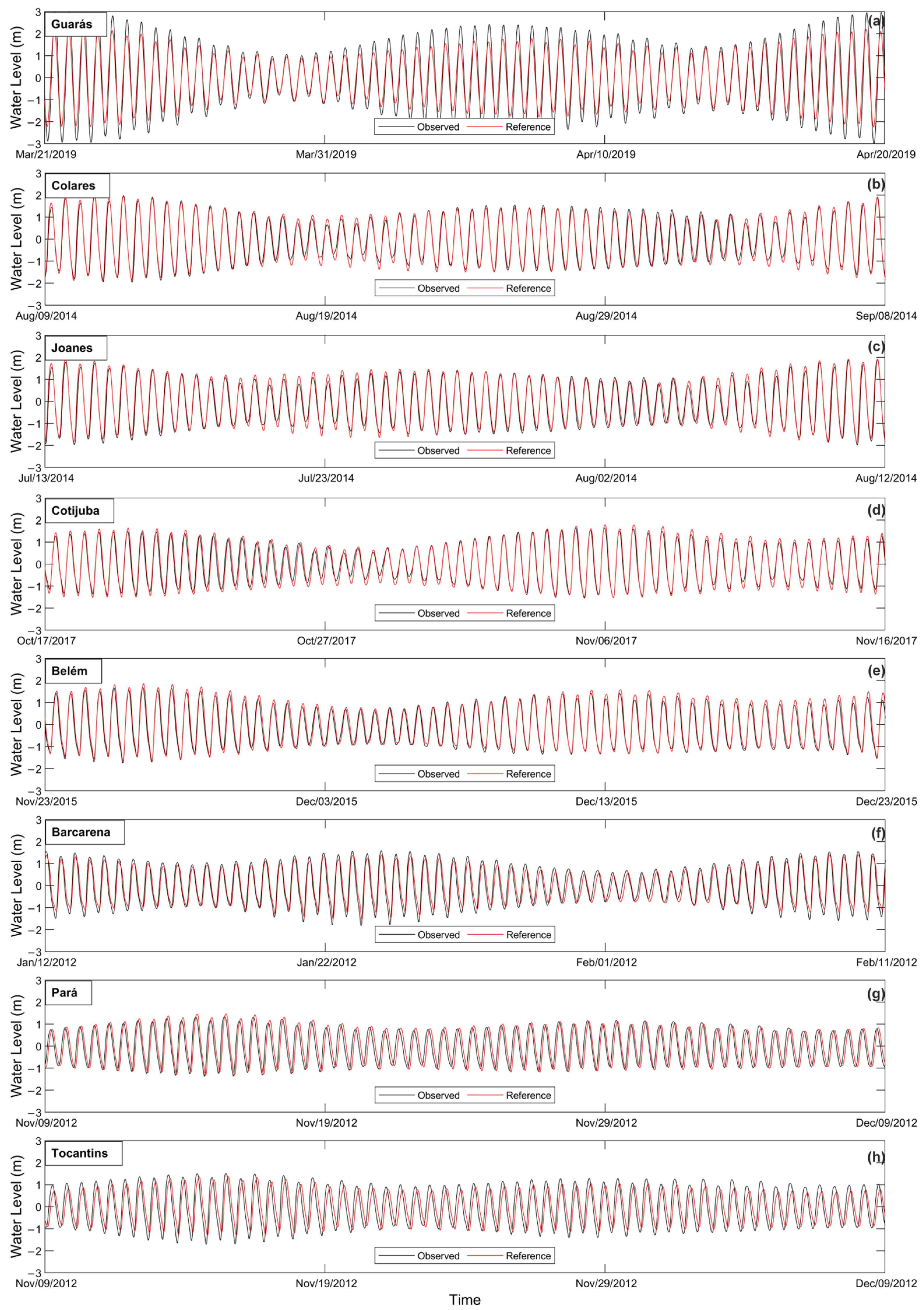
3.2. Reference Simulation

The hydrological model successfully simulated tidal elevations with a reasonable degree of accuracy, extending from the estuary mouth up to 200 km inland. The simulation captured the general tidal behavior, including the positive asymmetry upstream, which is characterized by rapid flood and slower ebb tides.

At the Guarás monitoring station, located at the estuary mouth, the model showed satisfactory results. The station’s performance metrics were an NSE of 0.88, an R² of 0.94, an RMSE of 0.49, an RRMSE of 8.06%, and a Bias of 0.24. The neap tide showed good agreement between the observed and modeled data (Figure 4a), but spring tides showed lower modeled amplitudes. While the observed spring tides reached ±3 m, the model only simulated around ±2.3 m.

Good results were found for the Colares, Joanes, Cotijuba, and Belém stations (Figure 4b–e). These stations showed RMSE, RRMSE, and Bias values below 0.3 m, 7%, and 0.1, respectively, while R² and NSE are above 0.9 (

Table 5. Metrics performance for stations situated in the Pará River estuary, where green represents good results, while orange represents poor results.

Station	RMSE (m)	RRMSE (%)	R2	NSE	Bias (m)
Guarás	0.49	8.08	0.94	0.89	0.24
Colares	0.20	4.47	0.96	0.96	0.04
Joanes	0.19	4.43	0.96	0.96	0.04
Cotijuba	0.21	6.49	0.95	0.93	0.05
Belém	0.21	5.51	0.95	0.94	0.04
Barcarena	0.30	8.28	0.88	0.88	0.09
Pará	0.46	15.98	0.65	0.61	0.21
Tocantins	0.57	16.87	0.55	0.54	0.32

).

The Barcarena station performed well in terms of NSE, R², and Bias, with values of 0.88, 0.88, and 0.09, respectively. However, the RMSE and RRMSE were slightly higher than at other stations, at 0.3 m and 8.28%. The errors increased due to the tidal phase lag of approximately 40 min. This phase lag becomes more pronounced as the tide progresses further inland (Figure 4f).

The Pará station had satisfactory R² and NSE values of 0.65 for both parameters, but poor values for RMSE, RRMSE, and Bias, at 0.46 m, 15.98%, and 0.21 m, respectively (Figure 4g). Similarly, the Tocantins station showed satisfactory NSE values but, overall, it performed poorly (Figure 4h). While the amplitude values were acceptable for the Pará and Tocantins stations, there was a significant delay between the modeled and observation data exceeding one hour, which lowered the goodness-of-fit metrics. This delay was caused by bathymetry inaccuracy, which is shallower than is required for this area. Table 5 shows the goodness-of-fit values for each station in the Pará River estuary.

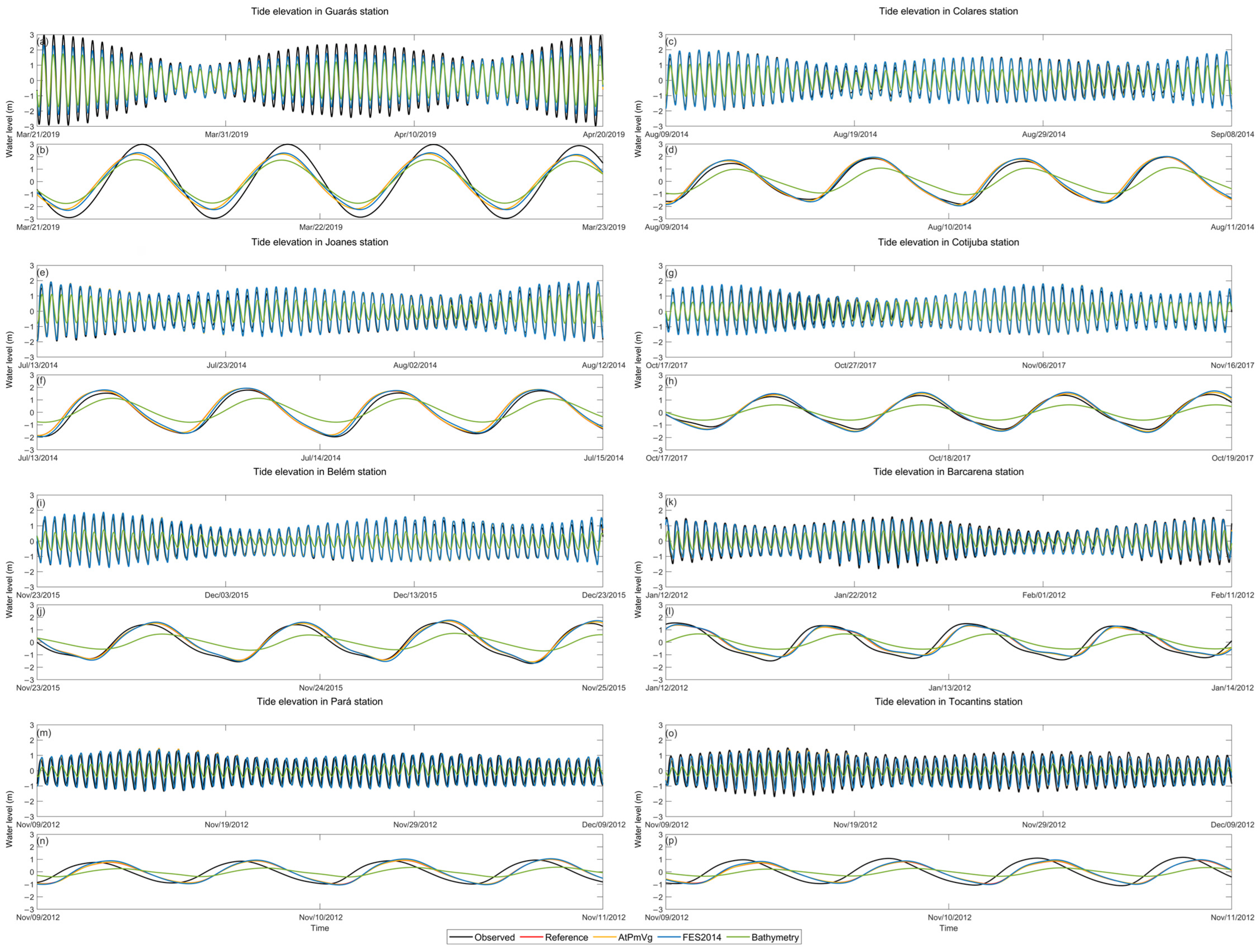
3.3. Scenario Performance

The Reference, AtPmVg, and FES2014 simulations had similar behavior across all stations (

Table 6. Goodness-of-fit values for each scenario across the eight stations available in the Pará River estuary. Green represents the best scenario result for each tidal station.

Station	Simulation	RMSE (m)	RRMSE (%)	R2	NSE	Bias (m)
Guarás	Reference	0.49	8.07	0.94	0.89	0.24
	AtPmVg	0.49	8.04	0.94	0.89	0.24
	FES2014	0.43	6.99	0.96	0.92	0.18
	Bathymetry	0.66	10.88	0.97	0.81	0.44
Colares	Reference	0.20	4.47	0.96	0.96	0.04
	AtPmVg	0.20	4.53	0.96	0.96	0.04
	FES2014	0.20	4.48	0.96	0.96	0.04
	Bathymetry	0.62	14.10	0.72	0.62	0.39
Joanes	Reference	0.19	4.43	0.96	0.96	0.04
	AtPmVg	0.19	4.45	0.96	0.96	0.04
	FES2014	0.20	4.47	0.96	0.96	0.04
	Bathymetry	0.65	14.90	0.67	0.57	0.42
Cotijuba	Reference	0.21	6.40	0.95	0.93	0.05
	AtPmVg	0.22	6.63	0.95	0.93	0.05
	FES2014	0.25	7.66	0.94	0.90	0.06
	Bathymetry	0.53	16.04	0.61	0.57	0.28
Belém	Reference	0.21	5.50	0.95	0.94	0.04
	AtPmVg	0.22	5.71	0.94	0.94	0.05
	FES2014	0.24	6.18	0.94	0.93	0.06
	Bathymetry	0.69	18.20	0.49	0.39	0.48
Barcarena	Reference	0.30	8.28	0.88	0.88	0.09
	AtPmVg	0.30	8.51	0.87	0.87	0.09
	FES2014	0.32	9.07	0.85	0.85	0.11
	Bathymetry	0.64	18.02	0.47	0.41	0.42
Pará	Reference	0.46	15.98	0.65	0.61	0.21
	AtPmVg	0.46	16.33	0.64	0.59	0.22
	FES2014	0.48	16.87	0.62	0.56	0.23
	Bathymetry	0.64	22.39	0.24	0.23	0.41
Tocantins	Reference	0.57	16.86	0.55	0.54	0.32
	AtPmVg	0.58	17.22	0.53	0.52	0.34
	FES2014	0.59	17.54	0.52	0.50	0.35
	Bathymetry	0.79	23.37	0.12	0.12	0.62

). Minimal differences were found mainly in FES2014, showing slightly higher amplitude and lag compared to the Reference and AtPmVg simulations. The Bathymetry scenario had the most significant impact on water levels, reducing tidal amplitudes at the Guarás station and showing even more pronounced decreases at the Pará and Tocantins stations. Figure 5 shows the tidal behavior of the stations across the scenarios.

At the Guarás station, the FES2014 scenario had better performance than the TPXO scenarios, obtaining an RMSE of 0.43 m, an RRMSE of 6.99%, a R² of 0.96, an NSE of 0.92, and a Bias of 0.18. Reference and AtPmVg simulations showed similar behavior, while the Bathymetry scenario had higher differences. The Bathymetry scenario produced RMSE, RRMSE, and Bias values of 0.66 m, 10.88%, and 0.44, respectively. However, the R² and NSE metrics showed good agreement, with values of 0.97 and 0.81, respectively.

For the Colares, Joanes, Cotijuba, and Belém stations, located between 55 km and 100 km inland, most scenarios had strong agreement with the observation data. Better results were found for the Reference simulation. The values for these four stations, considering the Reference, AtPmVg, and FES2014 scenarios, ranged from 0.19 m to 0.25 m for RMSE, 4.43% to 7.66% for RRMSE, 0.94 to 0.96 for R², 0.90 to 0.96 for NSE, and a Bias of 0.04 to 0.06. The Bathymetry scenario performed poorly, with unacceptable results.

Differences between the observed and modeled water levels increased progressively from Barcarena to Tocantins, located at 140 km and 200 km from the estuary mouth. Barcarena station showed satisfactory performance. The average goodness-of-fit values across the Reference, AtPmVg, and FES2014 scenarios were an RMSE of 0.31 m, an RRMSE of 8.62%, an R² of 0.87, an NSE of 0.87, and a Bias of 0.10.

All scenarios showed poor results for the Pará and Tocantins stations, with RRMSE values exceeding 15% and Bias values above 0.20 for all scenarios. Despite these challenges, the Reference, AtPmVg, and FES2014 scenarios still performed better than the Bathymetry scenario.

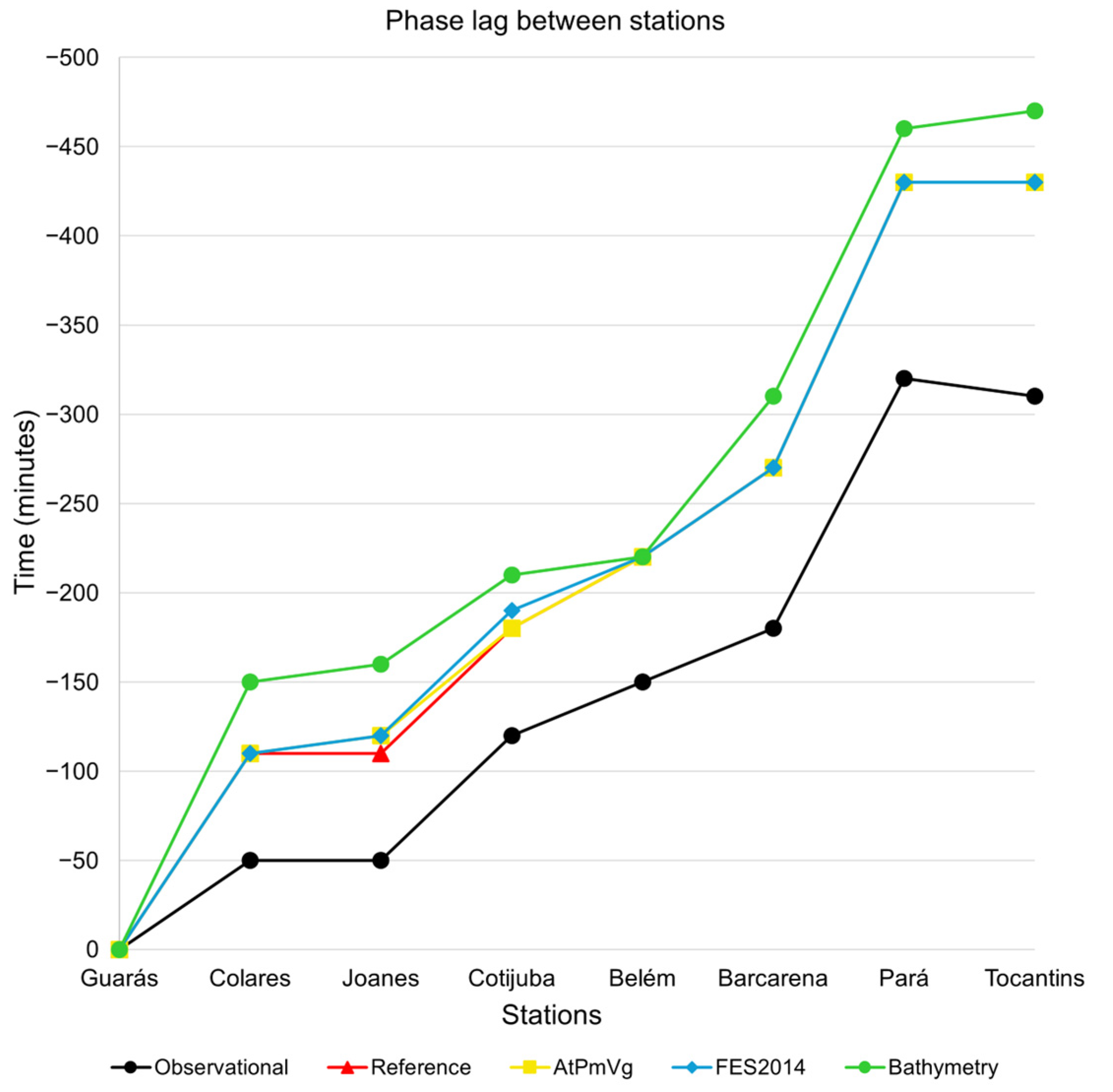
3.4. Tidal Wave Phase Lags

Differences were found in the time required for the wave to propagate between successive stations. Figure 6 shows the phase lag between stations in the Pará estuary, considering all simulations.

From the Guarás station, the observed tide requires −50 min to reach Colares and Joanes, while the simulations require more than −110 min. This pattern is repeated in all stations. To reach Cotijuba, Belém, and Barcarena, the observed tide needs −120 min to −180 min, while the models reach them in −180 to −310 min. The observed tide travels from Guarás to Pará and Tocantins in −320 min to −310 min, respectively, while the simulations require −430 to −470 min.

Despite the differences in absolute values, the general propagation trend across stations appears consistent among the models and observations, with increasing lag from Guarás to Pará and Tocantins.

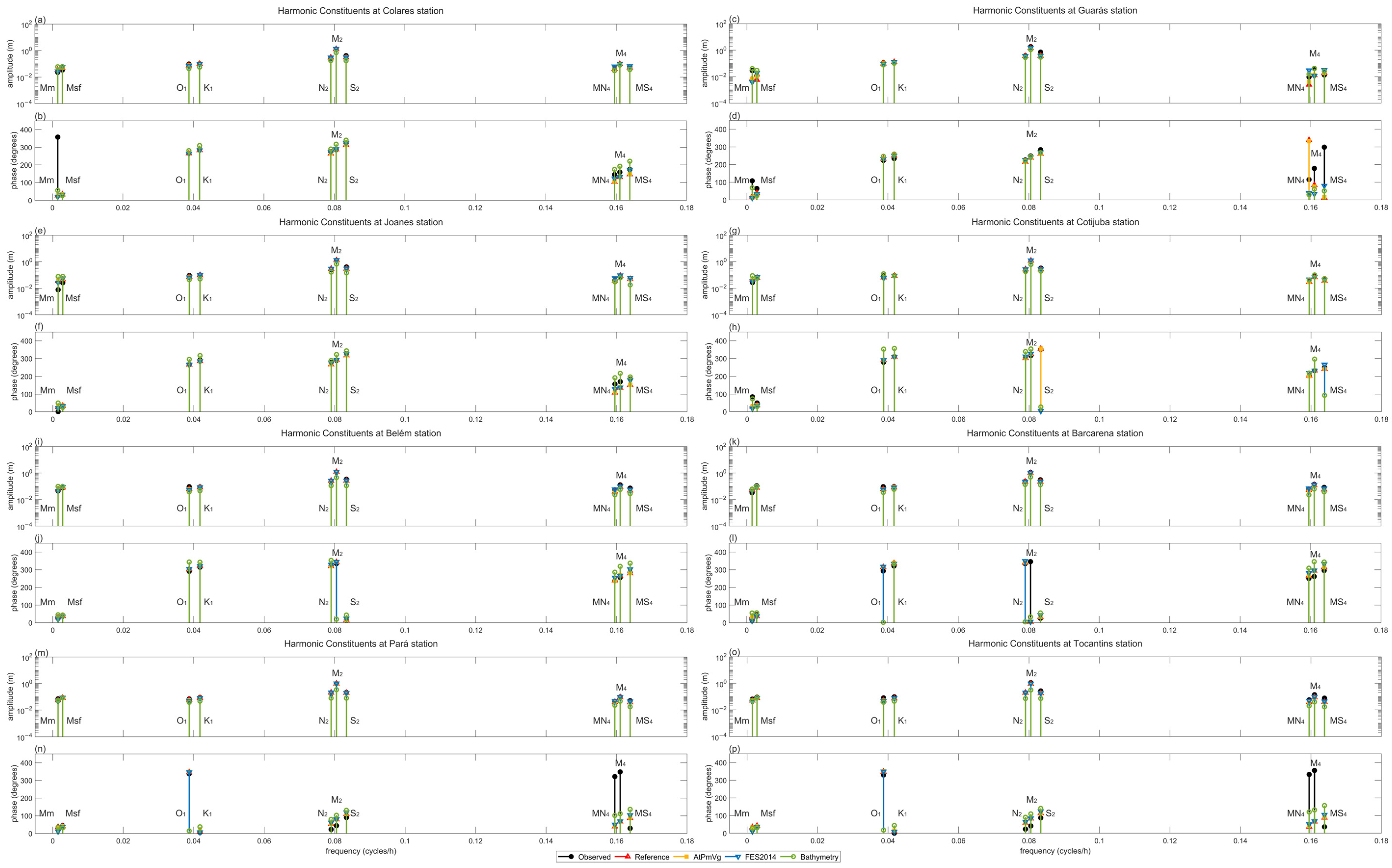
3.5. Harmonic Constituent Amplitude

Based on the harmonic analysis, the amplitudes and phase lags were calculated for eight tidal gauges. The hydrological model accurately simulated the amplitude of most components; however, it showed discrepancies for M₂ and, to a lesser extent, S₂, when compared to observations. Figure 7 shows the amplitude and phases of the main harmonic components for the eight tidal gauges and the scenarios.

Good results for M₂ were found for Colares, Joanes, Belém, Barcarena, and Pará, while the Guarás, Cotijuba, and Tocantins stations were less satisfactory. For the Guarás station, the observed M₂ amplitude was 1.85 m, while the Reference, AtPmVg, and FES2014 scenarios showed amplitudes ranging from 1.44 m to 1.52 m. The Bathymetry scenario showed a smaller amplitude of 1.10 m. Similar behavior was found at the Tocantins station, where the observed amplitude reached 1.11 m, while the Reference, AtPmVg, and FES2014 scenarios ranged from 0.91 m to 0.94, and the Bathymetry scenario reached 0.31 m.

The Cotijuba station was the only one where the modeled M₂ was higher than what was observed. While the observed M₂ was 1.06 m, the Reference, AtPmVg, and FES2014 scenarios ranged from 1.21 m to 1.26 m. Again, the Bathymetry scenario had a lower amplitude of 0.61 m, indicating a significant attenuation in the tidal wave in this scenario.

Among the simulations, Reference and AtPmVg exhibited nearly identical values across all available tidal components, with differences of only 0.01 m. As expected, the FES2014 simulation had higher differences, since the amplitudes are slightly higher. The maximum difference between the Reference and FES2014 simulations was observed at the Guarás station, where the M₂ component differed by 0.08 m.

The differences in the S₂ component were not significant. Larger differences between the modeled and observed values of S₂ were found in the Guarás, Colares, and Joanes stations. Those differences were below 0.4 m. Other component differences were below 0.12. This maximum value was found only in the Bathymetry scenario for the N₂ component.

3.6. Phases Lag in M₂

While amplitude discrepancies were found, the phase lag was the main factor impacting model accuracy. Given that M₂ is the dominant harmonic component in the domain, the phase lag in this component impacted the timing of water levels and the overall model performance. In phase lag, positive values were considered to represent earlier arrivals of the tide, while negative values were later arrivals. Figure 8 shows the delay of the stations for all the scenarios, considering the ranges to have good, satisfactory, and poor results for M₂.

Four stations—Guarás, Barcarena, Pará, and Tocantins—showed high phase lags, while Colares, Joanes, Cotijuba, and Belém had good agreement with the observation data. At the Guarás station, the modeled tide preceded the observation data by 20 min across most scenarios, except for the Bathymetry scenario, which had only a 6-min lag. As this station is positioned downstream, at the estuary mouth, a phase lag of 20 min is above that considered acceptable.

Barcarena, Pará, and Tocantins stations showed unacceptable phase lags in all scenarios. In terms of the Reference, AtPmVg, and FES2014 scenarios, the average delays were −40, −75, and −88 min for Barcarena, Pará, and Tocantins, respectively. For the Bathymetry scenario, the delays were more pronounced for those stations, with values ranging from −98 to −142 min.

For the Colares and Joanes stations, Reference, AtPmVg, and FES2014 scenarios showed good phase lag, with an average of −6 min for both stations. The Bathymetry scenario showed a delay of more than 60 min. At the Cotijuba and Belém stations, the phase lag remained within acceptable limits in most scenarios, averaging −20 and −18 min, respectively, for Reference, AtPmVg, and FES2014. However, the Bathymetry scenario showed longer delays of −76 min for Cotijuba and −94 min for Belém. Overall, the phase lag analysis showed that the Bathymetry scenario contained the greatest delays compared to other simulations, followed by FES2014, AtPmVg, and Reference.

4. Discussion

4.1. Boundary Conditions

Based on the literature, the level of agreement among ocean tide models varies according to the study area. For instance, Timko et al. [66] evaluated the results from the Hybrid Coordinate Ocean Model (HYCOM), TPXO8, and FES2014 models in regions including the Northwest European shelf, Hudson Bay, Hudson Strait, the Gulf of St. Lawrence, the Gulf of Maine, the Patagonian shelf, and the Northwest Australian shelf. While the focus was on HYCOM, the errors for many harmonic components (M₂, S₂, N₂, K₁, and O₁) in TPXO8 and FES2014 were similar, indicating consistency between the two models. Byrne et al. [67] also found that, overall, TPXO9 and FES2014 provided comparable results for 41 tide gauges in the United Kingdom, with observed errors typically around ±15 cm.

In contrast, Lee and Lee [68] and Fu et al. [69] reported better results for the FES2014 model compared with other global tidal models. Lee and Lee [68] evaluated five global tidal models—DTU10, EOT11a, FES2014, NAO99, and TPXO8—for 10 tidal gauges in the East Sea of Korea. Overall, TPXO showed the highest accuracy in K₁, and O₁; however, the FES2014 model showed the best accuracy across the four main components (M₂, S₂, K₁, and O₁).

Fu et al. [69] evaluated the accuracy of seven global models (DTU10, EOT11a, FES2014, GOT4.8, HAMTIDE12, OSU12, and TPXO8) against 37 tide gauge observations in the South China Sea. Fu et al. [69] found that the tidal models being evaluated showed higher precision in deep-water areas than in coastal areas, due to the influence of shoreline and water depth. Poor results were found at a water depth of less than 100 m. In coastal areas, the tidal model with lower root mean square (RMS) values for M₂, S₂, and N₂ was FES2014, compared to the other six tidal models. TPXO8 only showed the best results for K₁, while EOT11a showed the best results for O₁. Overall, the authors reported that the FES2014 model had the best performance among the other tidal models.

Gregg et al. [23] analyzed five global tidal models—FES2014b, EOT20, GOT4.10c, TPXO9-atlas-v5, and DTU16—focusing on a region spanning from 15° W to 10° E and 45° N to 65° N. Their findings indicated that TPXO9-atlas-v5 performed best when evaluated across all available sites. However, FES2014b yielded the most accurate results in locations where the tidal models did not assimilate observation data from tidal stations.

Ahn and Ronan [70] also implemented two different hydrodynamic models, the finite volume community ocean model (FVCOM) and the advanced circulation model (ADCIRC), using two global tide models, TPXO8 and FES2014, for the Shinnecock Bay area (United States of America). Both tide models generated similar amplitudes and phases for M₂, S_2, and N₂, while O₁ showed greater discrepancies. The authors concluded that the choice of hydrodynamic model software had more impact on the simulation than the choice of the tidal model as an open boundary. This suggests that while assessing tidal models is important for defining open boundaries, other internal parameters may have a greater impact on the accuracy and reliability of the simulations, such as different discrete algorithms being needed, different wet–dry point treatments being used to simulate inundation, and different bottom friction parameterization methods being utilized.

Thus, both the TPXO and FES models show good accuracy with observed results in different zones of the world. In this study, a strong agreement was found between the TPXO Regional Amazon Shelf 1/60° and FES2014 at the estuary model boundary, supporting the comparable performance of these two tidal models. Harmonic analysis revealed, overall, good agreement between the models, with minor differences in shallow water components such as MN₄ and MS₄. This suggests that both TPXO and FES2014 are suitable for representing tidal oscillation in the estuary. Both the Reference and FES2014 scenarios showed similar results when compared to eight tidal gauges in the Pará River estuary.

4.2. Explicit Simulation of Vegetation and Porous Media

The simulation of hydrological processes such as precipitation, evaporation, infiltration, exfiltration, and vegetation development had no significant impact on estuarine hydrodynamics, particularly on water levels. However, this experiment highlighted areas for future improvements in the MOHID-Land model code. One notable limitation is that the runoff module does not account for wind effects as MOHID-Land was initially designed to simulate soil–water–atmosphere interactions [35].

Wind is an important parameter of the water bodies’ hydrodynamic, influencing wind-generated waves, stress, and currents [71,72,73]. In estuaries, wind affects water levels, movement, and surface conditions [72]. While wind may have a lesser impact on the Pará River estuary, due to strong macro-tidal forces, its influence remains worth exploring. In other water bodies, like micro-tidal estuaries, lagoons, or lakes, wind is a key driver of circulation and mixing [73,74,75]. To ensure the broader applicability of the model, incorporating wind effects into the MOHID-Land surface runoff module could be considered in future developments.

Regarding soil processes, the exchanges between the estuary and the soil primarily affect the soil itself rather than the overall water levels in the estuary. The exchange of water from the soil to the estuary during ebb tides is relatively small compared to the forces and volumes involved in tidal fluctuations. The tide overshadows the smaller contributions from soil porewater discharge.

However, the exchange across the soil–water interface might become particularly important when modeling water quality conditions in the Pará River estuary. Factors such as salinity, nutrient levels, and temperature are greatly impacted by tidal fluctuation, evaporation, and precipitation [76,77,78]. Therefore, future simulations that incorporate these parameters are expected to provide a more comprehensive understanding of water exchanges in coastal zones.

4.3. Bathymetry Analysis

The model proved to be highly sensitive to bathymetry, with significantly worse performance by the Bathymetry scenario compared to the Reference scenario. This suggests that local characteristics have a greater impact on the model than the open boundary conditions or the activation of different hydrological processes. In hydrodynamic models, bathymetry significantly affects water level and flow dynamics. Calibration of bathymetric data has been shown to substantially enhance model performance, as evidenced in this study and corroborated by the findings of Cea and French [79] and Khanarmuei et al. [80].

Despite its critical role, the uncertainty associated with bathymetric data is often overlooked [79]. Both Cea and French [79] and Khanarmuei et al. [80] highlighted that calibrating the bathymetric data can significantly enhance tidal current simulations, demonstrating that the models are more sensitive to variations in bed elevation than to changes in the bed friction coefficient. Both studies also showed a higher sensitivity to currents in bathymetric calibration.

In this study, the impact of two distinct bathymetric configurations was analyzed using the MOHID-Land model. The Reference bathymetry underwent significant smoothing and removal of sandbanks at the estuary mouth, while the Bathymetry scenario used data originally developed for a hydrodynamic model and then interpolated into the MOHID-Land grid.

The simulations revealed notable differences in water levels between the two configurations. In the Bathymetry scenario, the tidal amplitude was substantially lower compared to both the Reference simulation and the observation data, indicating the need for calibration at the estuary mouth. The sandbanks, located at the estuary mouth in the Bathymetry scenario, acted as barriers that were responsible for a decrease in the tidal waves’ amplitude, resulting in a shallow water column and also delaying the tidal wave. The sandbanks prevented the tidal waves from reaching the Colares and Joanes stations within an acceptable time, delaying the wave by approximately 60 min. The increased friction dissipated the energy [81], which reduced the fluid velocity, slowed tidal wave propagation, and attenuated tidal amplitude. Sandbanks play a critical role in modulating tidal dynamics by increasing local friction, which directly impacts the energy and behavior of tidal waves [82,83].

In the Reference scenario, the removal of sandbanks caused faster tidal wave propagation, whereby the modeled water level preceded observations in the Guarás station, showing an excessive bathymetry alteration for this specific area. Although the scenarios showed phase lags, the statistical values for the Reference, AtPmVg, and FES2014 scenarios showed good results, mainly for Guarás, Colares, Joanes, Cotijuba, Belém, and Barcarena. The two inner stations, Pará and Tocantins, required more attention to the data and more calibration.

5. Conclusions

This research aimed to assess the ability of the MOHID-Land hydrological model to simulate macrotidal elevation in the Pará River estuary, while also evaluating the impact of other parameters and boundary conditions on model performance. The findings suggest that MOHID-Land can effectively simulate tidal oscillations with good accuracy across eight tidal stations, although the performance for stations further inland could be improved by enhanced bathymetry.

Both the TPXO Regional Amazon Shelf 1/60° and FES2014 tidal models provide comparable results in simulating tidal behavior in the estuary. Despite minor variations in specific harmonic components when compared with each other’s results, both models showed similar outcomes and good agreement in terms of the goodness-of-fit values. This supports the suitability of both tidal models for representing tidal behavior in the study area.

Hydrological processes, such as precipitation, evaporation, and the exchange from the soil layer to the estuary, had a minimal impact on water levels as tidal forces dominate the domain and represent larger volumes of water than exchanges with the terrestrial hydrological process. However, the experiment identified a limitation in the Runoff module of MOHID-Land, which, currently, does not consider the effect of wind on the water column. Incorporating wind effects in future versions could improve the model’s dynamic accuracy, especially for simulations in micro-tidal estuaries, lagoons, or lakes.

Bathymetry emerged as a critical factor influencing model performance. Sandbanks increased the local friction, impacting tidal wave energy and behavior. By using smoother bathymetry, the model reached accurate amplitudes and exhibited smaller phase lags.

In summary, the MOHID-Land model proved to be robust in simulating tidal dynamics in the Pará River estuary. Its capability extends to potential applications in future research aimed at understanding the exchange of various parameters between the land and coastal environments, including water, temperature, salinity, sediments, and nutrients. Incorporating these exchanges is crucial for future water-quality models, as the interactions between soil, groundwater, and estuarine waters are vital for understanding overall water quality.

References

1. Spyrakos, E.; O’Donnell, R.; Hunter, P.D.; Miller, C.; Scott, M.; Simis, S.G.H.; Neil, C.; Barbosa, C.C.F.; Binding, C.E.; Bradt, S.; et al. Optical types of inland and coastal waters. Limnol. Oceanogr. 2018, 63, 846–870. [Google Scholar] [CrossRef]
2. Cox, J.R.; Lingbeek, J.; Weisscher, S.A.H.; Kleinhans, M.G. Effects of Sea-Level Rise on Dredging and Dredged Estuary Morphology. J. Geophys. Res. Earth Surf. 2022, 127, e2022JF006790. [Google Scholar] [CrossRef]
3. Schrijvershof, R.A.; van Maren, D.S.; Van der Wegen, M.; Hoitink, A.J.F. Land Reclamation Controls on Multi-Centennial Estuarine Evolution. Earth’s Future 2024, 12, e2024EF005080. [Google Scholar] [CrossRef]
4. Wong, P.; Losada, I.; Gattuso, J.P.; Hinkel, J.; Khattabi, A.; McInnes, K.; Sallenger, A. Coastal Systems and Low-Lying Areas. In Climate Change 2014: Impacts, Adaptation, and Vulnerability. Part A: Global and Sectoral Aspects; Contribution of Working Group II to the Fifth Assessment Report of the Intergovernmental Panel on Climate Change; Cambridge University Press: Cambridge, UK, 2014; pp. 361–409. Available online: https://www.ipcc.ch/site/assets/uploads/2018/02/WGIIAR5-Chap5_FINAL.pdf (accessed on 4 February 2025).
5. Guo, J.; Ma, Y.; Ding, C.; Zhao, H.; Cheng, Z.; Yan, G.; You, Z. Impacts of Tidal Oscillations on Coastal Groundwater System in Reclaimed Land. J. Mar. Sci. Eng. 2023, 11, 2019. [Google Scholar] [CrossRef]
6. Abedin, M.A.; Habiba, U.; Shaw, R. Community Perception and Adaptation to Safe Drinking Water Scarcity: Salinity, Arsenic, and Drought Risks in Coastal Bangladesh. Int. J. Disaster Risk Sci. 2014, 5, 110–124. [Google Scholar] [CrossRef]
7. Tully, K.; Gedan, K.; Epanchin-Niell, R.; Strong, A.; Bernhardt, E.S.; BenDor, T.; Weston, N.B. The Invisible Flood: The Chemistry, Ecology, and Social Implications of Coastal Saltwater Intrusion. BioScience 2019, 69, 368–378. [Google Scholar] [CrossRef]
8. Kim, J.; Warnock, A.; Ivanov, V.Y.; Katopodes, N.D. Coupled modeling of hydrologic and hydrodynamic processes including overland and channel flow. Adv. Water Resour. 2012, 37, 104–126. [Google Scholar] [CrossRef]
9. Siqueira, V.A.; Paiva, R.C.D.; Fleischmann, A.S.; Fan, F.M.; Ruhoff, A.L.; Pontes, P.R.M.; Paris, A.; Calmant, S.; Collischonn, W. Toward continental hydrologic–hydrodynamic modeling in South America. Hydrol. Earth Syst. Sci. 2018, 22, 4815–4842. [Google Scholar] [CrossRef]
10. Beven, K. Causal models as multiple working hypotheses about environmental processes. Comptes Rendus Geosci. 2012, 344, 77–88. [Google Scholar] [CrossRef]
11. Okiria, E.; Okazawa, H.; Noda, K.; Kobayashi, Y.; Suzuki, S.; Yamazaki, Y. A comparative evaluation of lumped and semi-distributed conceptual hydrological models: Does model complexity enhance hydrograph prediction? Hydrology 2022, 9, 89. [Google Scholar] [CrossRef]
12. Devi, G.K.; Ganasri, B.P.; Dwarakish, G.S. A review on hydrological models. Aquat. Procedia 2015, 4, 1001–1007. [Google Scholar] [CrossRef]
13. Suhana, M.P.; Nursyahnita, S.D.; Idris, F. Hydrodynamic model approach to study the pattern of sea surface currents around the Tanjungpinang City reclamation site. IOP Conf. Ser. Earth Environ. Sci. 2023, 1148, 012014. [Google Scholar] [CrossRef]
14. Liu, Z.; Zhang, H.; Liang, Q. A coupled hydrological and hydrodynamic model for flood simulation. Hydrol. Res. 2019, 50, 589–606. [Google Scholar] [CrossRef]
15. Mansanarez, V.; Thirel, G.; Delaigue, O.; Liquet, B. Development of a semi-distributed hydrological model on a tidal-affected river: Application to the Adour catchment, France. In Proceedings of the EGU General Assembly 2020, Online, 4–8 May 2020; Available online: https://meetingorganizer.copernicus.org/EGU2020/EGU2020-13582.html (accessed on 4 February 2025). [CrossRef]
16. Lobligeois, F.; Andréassian, V.; Perrin, C.; Tabary, P.; Loumagne, C. When does higher spatial resolution rainfall information improve streamflow simulation? An evaluation using 3620 flood events. Hydrol. Earth Syst. Sci. 2014, 18, 575–594. [Google Scholar] [CrossRef]
17. Zhang, Y.; Li, W.; Sun, G.; Miao, G.; Noormets, A.; Emanuel, R.; King, J.S. Understanding coastal wetland hydrology with a new regional-scale, process-based hydrological model. Hydrol. Process. 2018, 32, 3158–3173. [Google Scholar] [CrossRef]
18. Qu, Y.; Duffy, C.J. A semidiscrete finite volume formulation for multiprocess watershed simulation. Water Resour. Res. 2007, 43, 08419. [Google Scholar] [CrossRef]
19. Brito, D.; Campuzano, F.J.; Sobrinho, J.; Fernandes, R.; Neves, R. Integrating operational watershed and coastal models for the Iberian Coast: Watershed model implementation—A first approach. Estuar. Coast. Shelf Sci. 2015, 167, 138–146. [Google Scholar] [CrossRef]
20. Hascoet, T.; Pellet, V.; Aires, F.; Takiguchi, T. Learning Global Evapotranspiration Dataset Corrections from a Water Cycle Closure Supervision. Remote Sens. 2023, 16, 170. [Google Scholar] [CrossRef]
21. Brouwer, C.; Goffeau, A.; Heibloem, M. Irrigation Water Management: Training Manual No. 1—Introduction to Irrigation; FAO—Food And Agriculture Organization of the United Nations: Rome, Italy, 1985; Available online: https://www.fao.org/4/r4082e/r4082e00.htm#Contents (accessed on 4 February 2025).
22. Bot, A.; Benites, J. The Importance of Soil Organic Matter: Key to Drought-Resistant Soil and Sustained Food Production; FAO—Food And Agriculture Organization of the United Nations: Rome, Italy, 2005; Available online: https://www.fao.org/4/a0100e/a0100e00.htm#Contents (accessed on 4 February 2025).
23. Gregg, D.E.; Penna, N.T.; Jones, C.; Maqueda, M.A.M. Accuracy assessment of recent global ocean tide models in coastal waters of the European North West Shelf. Ocean Model. 2024, 192, 102448. [Google Scholar] [CrossRef]
24. Ray, R.D.; Egbert, G.D.; Erofeeva, S.Y. Tide Predictions in Shelf and Coastal Waters: Status and Prospects. In Coastal Altimetry Coastal Altimetry; Vignudelli, S., Kostianoy, A., Cipollini, P., Benveniste, J., Eds.; Springer: Berlin/Heidelberg, Germany, 2010; pp. 191–216. [Google Scholar] [CrossRef]
25. Steinigeweg, C.S.; Paul, M.; Kleyer, M.; Schröder, B. Conquering new frontiers: The effect of vegetation establishment and environmental interactions on the expansion of tidal marsh systems. Estuaries Coasts 2023, 46, 1515–1535. [Google Scholar]
26. Allen, G.P.; Salomon, J.C.; Bassoullet, P.; Du Penhoat, Y.; de Grandpré, C. Effects of tides on mixing and suspended sediment transport in macrotidal estuaries. Sediment. Geol. 1980, 26, 69–90. [Google Scholar] [CrossRef]
27. Moraes, B.C.; Costa, J.M.N.; Costa, A.C.L.; Costa, M.H. Variação Espacial e Temporal da Precipitação no Estado do Pará. Acta Amaz. 2005, 35, 207–214. [Google Scholar] [CrossRef]
28. Gregório, A.M.D.S.; Mendes, A.C. Batimetria e Sedimentologia da Baía do Guajará, Belém, Estado do Pará, Brasil. Amaz. Ciênc. Desenvolv. 2009, 5, 53–72. Available online: https://repositorio.museu-goeldi.br/handle/mgoeldi/369 (accessed on 4 February 2025).
29. Ministério do Meio Ambiente (MMA). Caderno da Região Hidrográfica do Tocantins-Araguaia. Brasilia, 132p. 2006. Available online: https://www.mma.gov.br/estruturas/161/_publicacao/161_publicacao02032011035943.pdf (accessed on 27 June 2022).
30. Prestes, Y.O.; Borba, T.A.C.; Silva, A.C.; Rollnic, M. A Discharge Stationary Model for the Pará-Amazon Estuarine System. J. Hydrol. Reg. Stud. 2020, 28, 100668. [Google Scholar] [CrossRef]
31. Barthem, R.B.; Schwassmann, H.O. Amazon River Influence on the Seasonal Displacement of the Salt Wedge in the Tocantins River Estuary, Brazil, 1983-1985. Bol. Mus. Para. Emílio Goeldi. Sér. Zool. 1994, 10, 19–130. Available online: https://repositorio.museu-goeldi.br/handle/mgoeldi/496 (accessed on 4 February 2025).
32. Prestes, Y.O.; Silva, A.C.; Rollnic, M.; Rosário, R.P. The M2 and M4 Tides in the Pará River Estuary. Trop. Oceanogr. 2017, 45, 1679–3013. [Google Scholar] [CrossRef]
33. Rollnic, M.; Rosário, R.P. Tide propagation in tidal courses of the Pará river estuary, Amazon Coast, Brazil. J. Coast. Res. 2013, 165, 1581–1586. [Google Scholar] [CrossRef]
34. MOHID Wiki. Mohid Land. Available online: http://wiki.mohid.com/index.php?title=Mohid_Land (accessed on 27 June 2022).
35. Oliveira, A.R.; Ramos, T.B.; Simionesei, L.; Pinto, L.; Neves, R. Sensitivity Analysis of the MOHID-Land Hydrological Model: A Case Study of the Ulla River Basin. Water 2020, 12, 3258. [Google Scholar] [CrossRef]
36. Oliveira, A.R.; Ramos, T.B.; Pinto, L.; Neves, R. Direct integration of reservoirs’ operations in a hydrological model for streamflow estimation: Coupling a CLSTM model with MOHID-Land. Hydrol. Earth Syst. Sci. 2023, 27, 3875–3893. [Google Scholar] [CrossRef]
37. Ramos, T.B.; Simionesei, L.; Jauch, E.; Almeida, C.; Neves, R. Modelling soil water and maize growth dynamics influenced by shallow groundwater conditions in the Sorraia Valley region, Portugal. Agric. Water Manag. 2017, 185, 27–42. [Google Scholar] [CrossRef]
38. Mualem, Y. A new model for predicting the hydraulic conductivity of unsaturated porous media. Water Resour. Res. 1976, 12, 513–522. [Google Scholar] [CrossRef]
39. Van Genuchten, M.T. A closed-form equation for predicting the hydraulic conductivity of unsaturated soils. Soil Sci. Soc. Am. J. 1980, 44, 892–898. [Google Scholar] [CrossRef]
40. Allen, R.G.; Pereira, L.S.; Raes, D.; Smith, M. Crop Evapotranspiration—Guidelines for Computing Crop Water Requirements. In FAO Irrigation & Drainage Paper 56; Food and Agriculture Organization (FAO): Rome, Italy, 1998. [Google Scholar]
41. Ritchie, J.T. Model for predicting evaporation from a row crop with incomplete cover. Water Resour. Res. 1972, 8, 1204–1213. [Google Scholar] [CrossRef]
42. Egbert, G.D.; Erofeeva, S.Y. Efficient inverse modeling of barotropic ocean tides. J. Atmos. Ocean. Technol. 2002, 19, 183–204. [Google Scholar] [CrossRef]
43. Borba, T.A.C.; Rollnic, M. Runoff quantification on Amazonian Estuary based on hydrodynamic model. J. Coast. Res. 2016, 75, 43–47. [Google Scholar] [CrossRef]
44. Rosário, R.P.; Borba, T.A.C.; Santos, A.S.; Rollnic, M. Variability of Salinity in Pará River Estuary: 2D Analysis with Flexible Mesh Model. J. Coast. Res. 2016, 75, 128–132. [Google Scholar] [CrossRef]
45. Mendes, J.; Leitão, P.; Chambel Leitão, J.; Bartolomeu, S.; Rodrigues, J.; Dias, J.M. Improvement of an operational forecasting system for extreme tidal events in Santos Estuary (In Brazil). Geosciences 2019, 9, 511. [Google Scholar] [CrossRef]
46. Cancio, N.C.; Pierini, J.O. Suspended sediment transport in Rio Colorado agricultural basin, Argentina. Front. Built Environ. 2023, 9, 1142671. [Google Scholar] [CrossRef]
47. Brazilian Sea Observatory. AM_PA_2D. Available online: https://github.com/Brazilian-Sea-Observatory/AM_PA_2D (accessed on 21 May 2024).
48. United States Geological Survey (USGS). Earth Explore. Available online: https://earthexplorer.usgs.gov/ (accessed on 1 October 2022).
49. Marinha do Brasil. Cartas Raster. Available online: https://www.marinha.mil.br/chm/dados-do-segnav/cartas-raster (accessed on 27 March 2023).
50. Copernicus European Eyes on Earth. Global Land Cover. Available online: https://lcviewer.vito.be/download (accessed on 23 July 2024).
51. MapBiomas. Coleções MapBiomas. Available online: https://brasil.mapbiomas.org/colecoes-mapbiomas/ (accessed on 23 July 2024).
52. Batjes, N.H. SOTER-Based Soil Parameter Estimates for Latin America and the Caribbean (Ver. 1.0). ISRIC–World Soil Information, Wageningen, 2005. Available online: https://isric.org/sites/default/files/isric_report_2005_02.pdf (accessed on 23 July 2024).
53. Agência Nacional das Águas (ANA). HIDROWEB. Available online: https://www.snirh.gov.br/hidroweb/ (accessed on 25 May 2022).
54. United States Department of Agriculture (USDA); Soil Science Division Staff. Soil Survey Manual. In USDA Handbook 18; Ditzler, C., Scheffe, K., Monger, H.C., Eds.; Government Printing Office: Washington, DC, USA, 2017. Available online: https://www.nrcs.usda.gov/resources/guides-and-instructions/soil-survey-manual (accessed on 23 July 2024).
55. Handbook 60 (HB60). Rosetta, Estimate Unsaturated Soil Hydraulic Parameters from Soil Characterization Data. Available online: https://www.handbook60.org/rosetta/ (accessed on 23 July 2024).
56. Hersbach, H.; Bell, B.; Berrisford, P.; Biavati, G.; Horányi, A.; Muñoz Sabater, J.; Nicolas, J.; Peubey, C.; Radu, R.; Rozum, I.; et al. ERA5 Hourly Data on Single Levels from 1959 to Present. Copernicus Climate Change Service (C3S) Climate Data Store (CDS) 2018. Available online: https://doi.org/10.24381/cds.adbb2d47 (accessed on 1 March 2023).
57. Pereira, D.R.; Oliveira, A.R.; Costa, M.S.; Ramos, T.B.; Rollnic, M.; Neves, R.J. Evaluation of precipitation products in a Brazilian watershed: Tocantins-Araguaia watershed case study. Theor. Appl. Climatol. 2024, 155, 7845–7865. [Google Scholar] [CrossRef]
58. Agência Nacional de Águas (ANA). Sistema Interligado Nacional, Bacia do rio Tocantins, Reservatórios. Available online: https://www.ana.gov.br/sar/sin/b_tocantins/# (accessed on 16 February 2023).
59. Erofeeva, S.; Padman, L.; Howard, S.L. Tide Model Driver (TMD) Version 2.5, Toolbox for Matlab. GitHub 2020. Available online: https://www.github.com/EarthAndSpaceResearch/TMD_Matlab_Toolbox_v2.5 (accessed on 1 April 2023).
60. Centre National d’Études Spatiales (CNES). Aviso-FES. Available online: https://github.com/CNES/aviso-fes/tree/main (accessed on 30 July 2024).
61. Amazon Coastal Observatory (OCA). OCA Observational. Available online: https://oca.eco.br/en/banco-de-dados/oca-observa/ (accessed on 20 May 2022).
62. Pawlowicz, R.; Beardsley, B.; Lentz, S. Classical tidal harmonic analysis including error estimates in MATLAB using T_TIDE. Comput. Geosci. 2002, 28, 929–937. [Google Scholar] [CrossRef]
63. Moriasi, D.N.; Arnold, J.G.; Van Liew, M.W.; Bingner, R.L.; Harmel, R.D.; Veith, T.L. Model evaluation guidelines for systematic quantification of accuracy in watershed simulations. Trans. ASABE 2007, 50, 885–900. [Google Scholar] [CrossRef]
64. Moriasi, D.N.; Gitau, M.W.; Pai, N.; Daggupati, P. Hydrologic and water quality models: Performance measures and evaluation criteria. Trans. ASABE 2015, 58, 1763–1785. [Google Scholar] [CrossRef]
65. Williams, J.J.; Esteves, L.S. Guidance on setup, calibration, and validation of hydrodynamic, wave, and sediment models for shelf seas and estuaries. Adv. Civ. Eng. 2017, 2017, 1–25. [Google Scholar] [CrossRef]
66. Timko, P.G.; Timko, P.G.; Arbic, B.K.; Hyder, P.; Richman, J.G.; Zamudio, L.; O’Dea, E.; Wallcraft, A.J.; Shriver, J. F Assessment of shelf sea tides and tidal mixing fronts in a global ocean model. Ocean Model. 2019, 136, 66–84. [Google Scholar] [CrossRef]
67. Byrne, D.; Horsburgh, K.; O’Neill, C.K. Sensitivity of AMM15-Surge to Varying Tidal Boundary Conditions and Bottom Friction Coefficients. Res. Consult. Rep. 2019, 71, 33. Available online: https://eprints.soton.ac.uk/434878/1/NOC_R_C_71_Final.pdf (accessed on 3 November 2023).
68. Lee, J.C.; Lee, D.H. Accuracy assessment of recent global ocean tide models using tide gauge measurements from the East Sea of Korea. J. Coast. Res. 2022, 39, 354–359. [Google Scholar] [CrossRef]
69. Fu, Y.; Feng, Y.; Zhou, D.; Zhou, X.; Li, J.; Tang, Q. Accuracy assessment of global ocean tide models in the South China Sea using satellite altimeter and tide gauge data. Acta Oceanol. Sin. 2020, 39, 1–10. [Google Scholar] [CrossRef]
70. Ahn, J.E.; Ronan, A.D. Impact of discrepancies between global ocean tide models on tidal simulations in the Shinnecock Bay area. J. Waterw. Port Coast. Ocean Eng. 2019, 145, 04018042. [Google Scholar] [CrossRef]
71. Ahsan, Q.; Blumberg, A.F.; Thuman, A.J.; Gallagher, T.W. Geomorphological and meteorological control of estuarine processes: A three-dimensional modeling analysis. J. Hydraul. Eng. 2005, 131, 259–272. [Google Scholar] [CrossRef]
72. Cho, H.J. Effects of prevailing winds on turbidity of a shallow estuary. Int. J. Environ. Res. Public Health 2007, 4, 185–192. [Google Scholar] [CrossRef]
73. Chen, F.; Zhang, C.; Brett, M.T.; Nielsen, J.M. The importance of the wind-drag coefficient parameterization for hydrodynamic modeling of a large shallow lake. Ecol. Inform. 2020, 59, 101106. [Google Scholar] [CrossRef]
74. Llebot, C.; Rueda, F.J.; Solé, J.; Artigas, M.L.; Estrada, M. Hydrodynamic states in a wind-driven microtidal estuary (Alfacs Bay). J. Sea Res. 2014, 85, 263–276. [Google Scholar] [CrossRef]
75. Kjerfve, B.; Magill, K.E. Geographic and hydrodynamic characteristics of shallow coastal lagoons. Mar. Geol. 1989, 88, 187–199. [Google Scholar] [CrossRef]
76. Wilson, A.M.; Gardner, L.R. Tidally driven groundwater flow and solute exchange in a marsh: Numerical simulations. Water Resour. Res. 2006, 42, W01405. [Google Scholar] [CrossRef]
77. Wilson, A.M.; Morris, J.T. The influence of tidal forcing on groundwater flow and nutrient exchange in a salt marsh-dominated estuary. Biogeochemistry 2012, 108, 27–38. [Google Scholar] [CrossRef]
78. Xin, P.; Yu, X.; Zhan, L.; Cheng, H.; Yuan, S. Surface water-groundwater interaction affects soil temperature distributions and variations in salt marshes. Adv. Water Resour. 2023, 172, 104366. [Google Scholar] [CrossRef]
79. Cea, L.; French, J.R. Bathymetric error estimation for the calibration and validation of estuarine hydrodynamic models. Estuar. Coast. Shelf Sci. 2012, 100, 124–132. [Google Scholar] [CrossRef]
80. Khanarmuei, M.; Suara, K.; Sumihar, J.; Brown, R.J. Hydrodynamic modelling and model sensitivities to bed roughness and bathymetry offset in a micro-tidal estuary. J. Hydroinform. 2020, 22, 1536–1553. [Google Scholar] [CrossRef]
81. Knaapen, M.A. Sandbank occurrence on the Dutch continental shelf in the North Sea. Geo-Mar. Lett. 2009, 29, 17–24. [Google Scholar] [CrossRef]
82. Pattiaratchi, C.; Collins, M. Mechanisms for linear sandbank formation and maintenance in relation to dynamical oceanographic observations. Prog. Oceanogr. 1987, 19, 117–176. [Google Scholar] [CrossRef]
83. Sothmann, J.; Schuster, D.; Kappenberg, J.; Ohle, N. Efficiency of artificial sandbanks in the mouth of the Elbe estuary for damping the incoming tidal energy. In Proceedings of the 5th International Short Conference on Applied Coastal Research (SCACR 2011), Aachen, Germany, 6–9 June 2011. [Google Scholar]
Figure 1. Map of the study area and the model domain in the Pará River estuary, showing the distribution of tidal stations as blue points. Red points indicate locations where tidal data were extracted from global models. The tidal boundary is represented in dark blue, while the model limits are shown in light blue.
Water 17 01048 g001
Figure 2. Bathymetry applied in the Pará River estuary model. (a) Reference bathymetry, using in situ data and nautical charts; (b) Brazilian Sea Observatory [47] bathymetry, developed for a hydrodynamic model; and (c) the difference map between the Reference and the Brazilian Sea Observatory [47] bathymetries.
Water 17 01048 g002
Figure 3. MOHID-Land input data: (a) land cover information available from MapBiomas for the year 2010; (b) roughness map derived from Copernicus Land Cover; (c) soil classifications, based on USDA textures.
Water 17 01048 g003
Figure 4. Observation and modeled data for the tidal stations. Black lines represent observation data, and red lines represent the Reference model.
Water 17 01048 g004
Figure 5. Water level at each tidal station, for one month, and the first two days for better visualization. Black line—observation data, red line—Reference, yellow line—AtPmVg, light blue line—FES2014, and green line—Bathymetry simulation.
Water 17 01048 g005
Figure 6. Phase lag of the tidal wave between successive stations in the Pará estuary, comparing the observation data with different simulation models. Black line with circles—observation data; red line with triangles—Reference; yellow line with squares—AtPmVg; blue line with diamonds—FES2014; green line with circles—Bathymetry model.
Water 17 01048 g006
Figure 7. Amplitude and phases for the main harmonic constituents from tidal stations, comparing the observation data and modeled results. Black line—the observation data; red line—Reference; yellow line—AtPmVg; blue line—FES2014; green line—Bathymetry model.
Water 17 01048 g007
Figure 8. Phase lags in the Pará River estuary, considering the differences between simulations.
Water 17 01048 g008