

Detection and Characterization of Marine Ecotones Using Satellite-Derived Environmental Indicators
 , ,
, ,
Abstract
1. Introduction
2. Materials and Methods
2.1. Data Source
2.2. Study Area
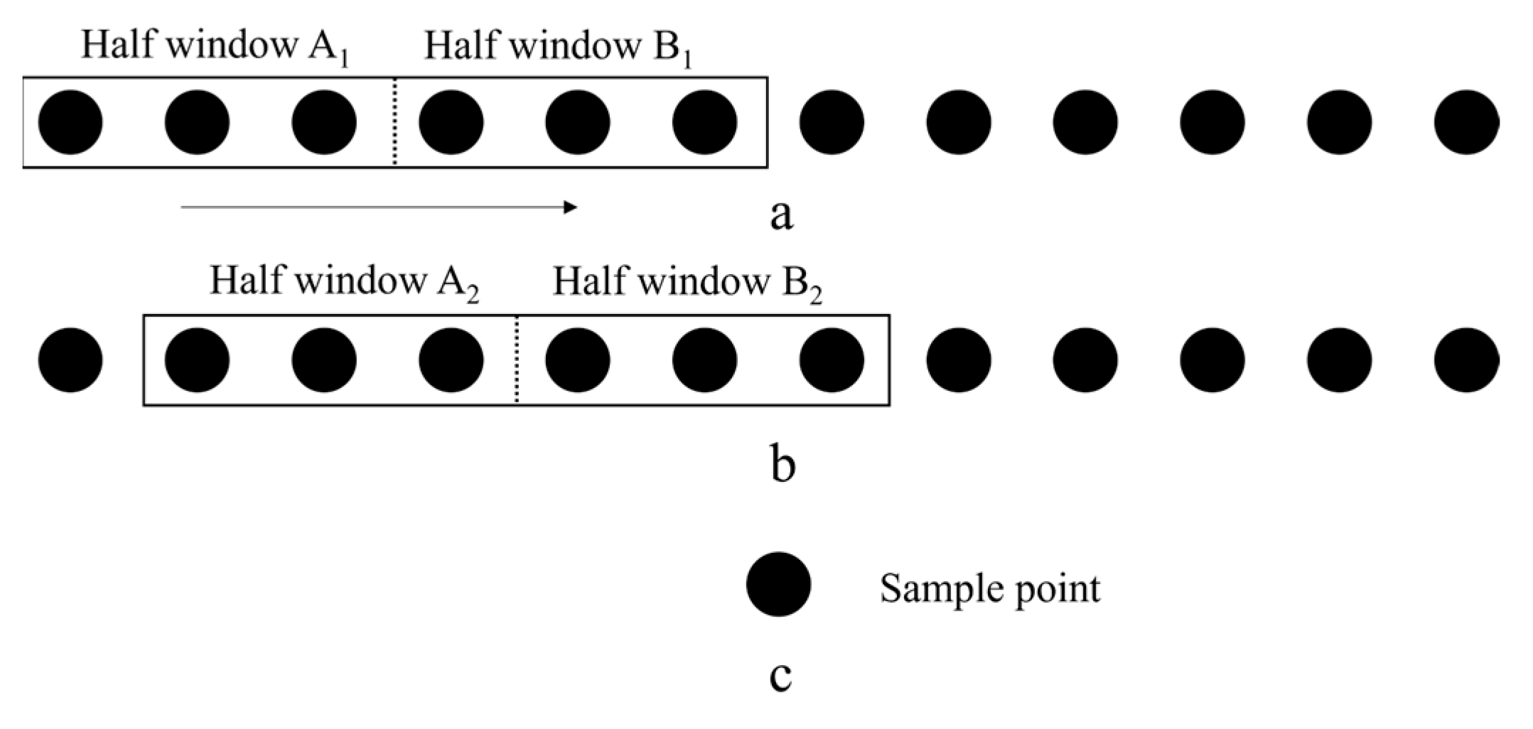
2.3. MSW Method
2.4. Selection of Dissimilarity Coefficient
2.5. Selection of Variable
3. Results
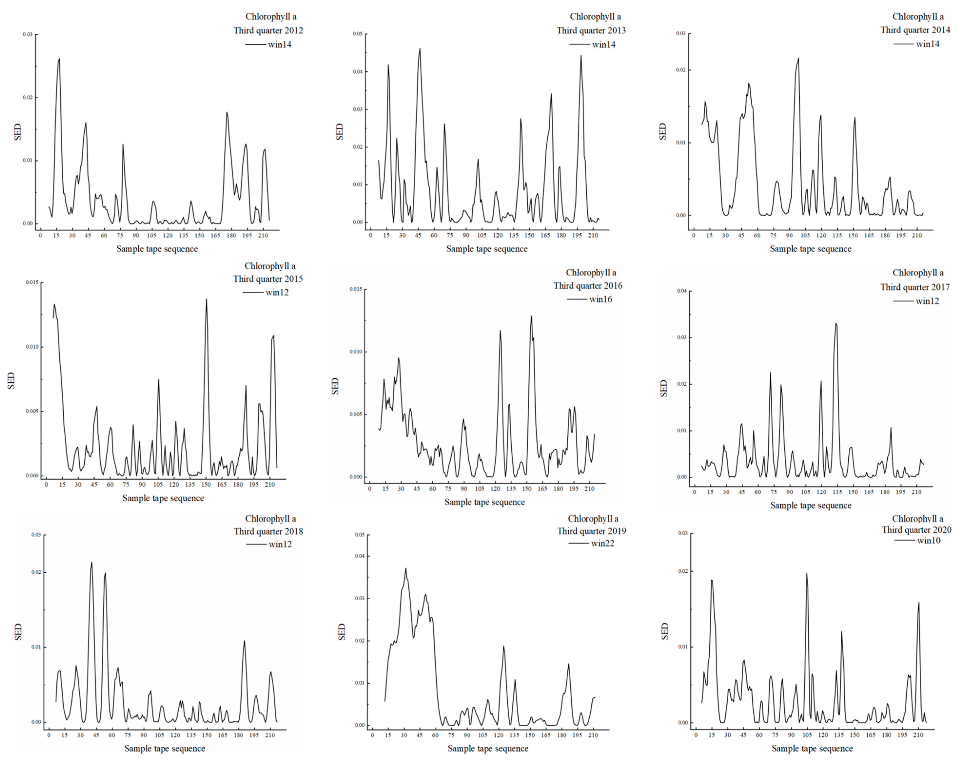
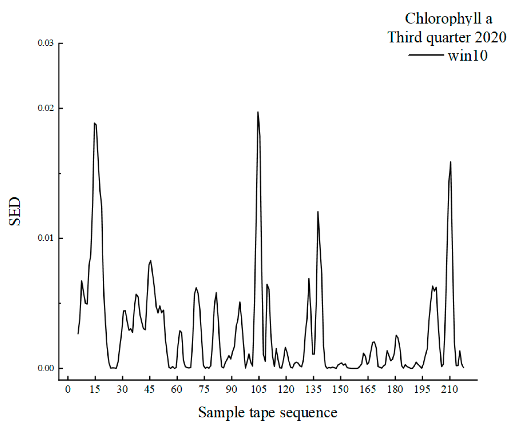
3.1. MSW Based on Chlorophyll-a
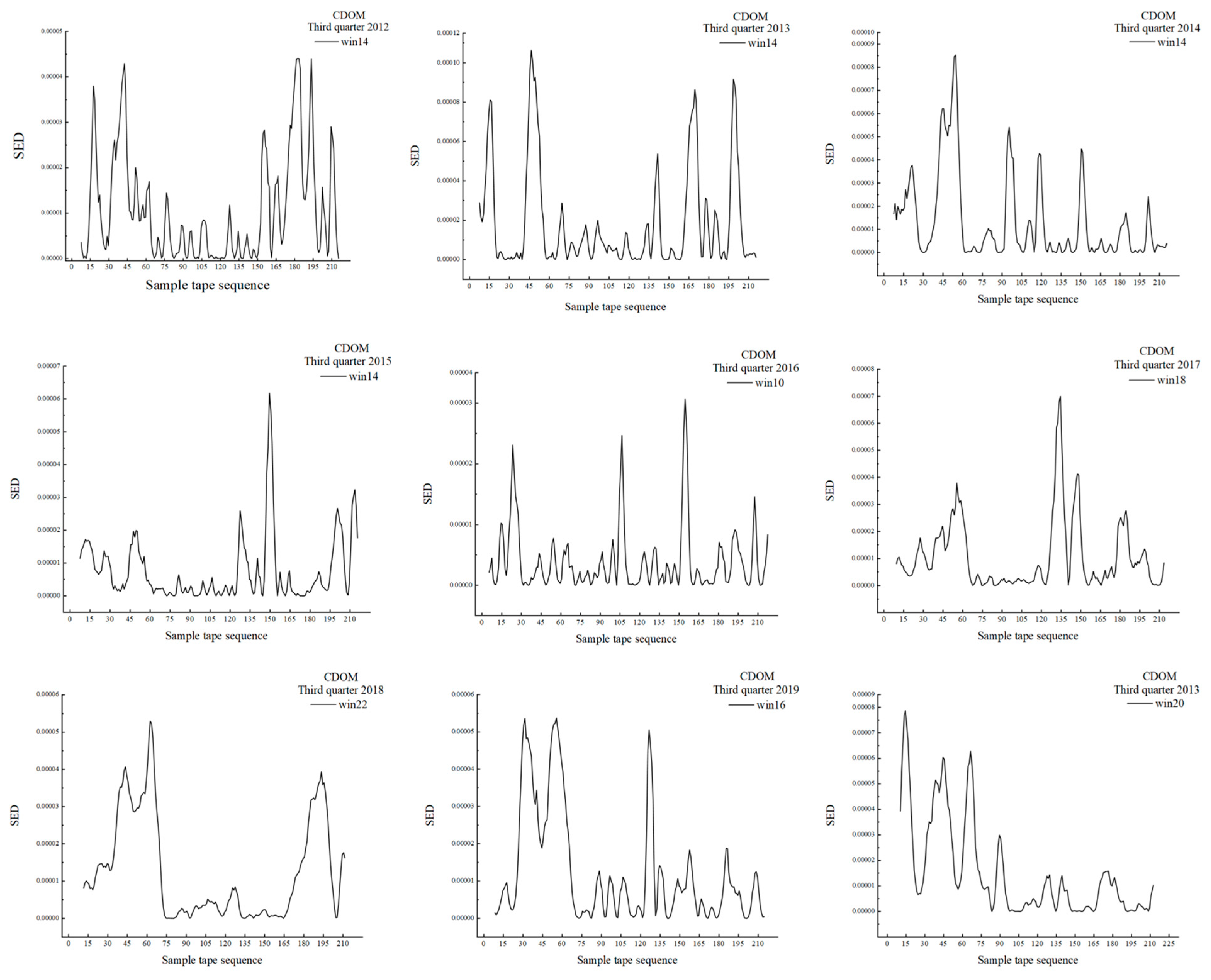
3.2. MSW Based on CDOM
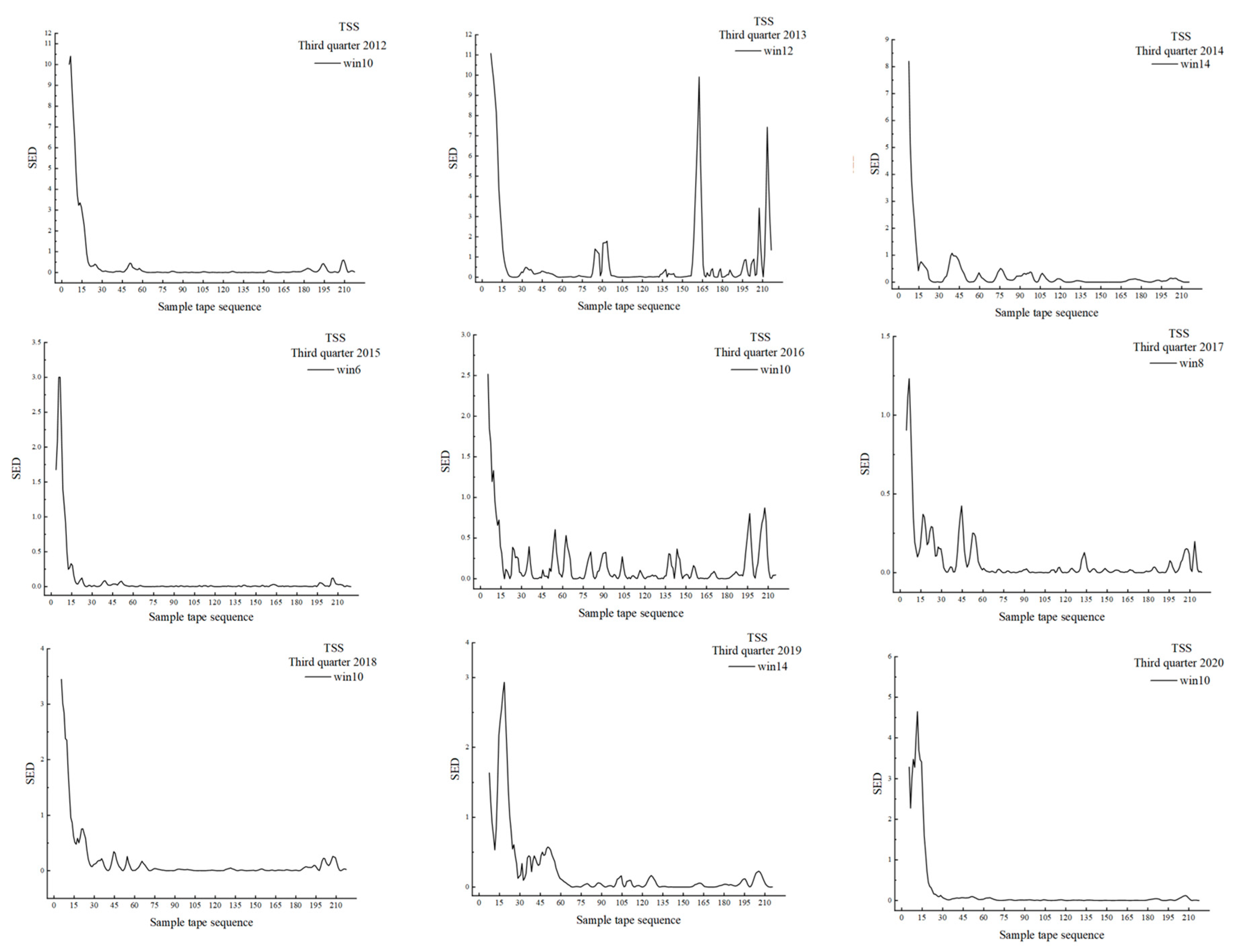
3.3. The Results of MSW Based on TSS
4. Discussion
4.1. Defect of MSW Method and Data
4.2. Strength of GOCI Data and Position of Sample Belt
4.3. Practical Applications of Result
5. Conclusions
Author Contributions
Funding
Data Availability Statement
Conflicts of Interest
References
- Cheng, H.Q.; Chen, J.Y. Study on the Impact of Sea Level Rise on the Estuary of Yangtze River; Science Press: Beijing, China, 2016. (In Chinese) [Google Scholar]
- Kline, J.D.; Swallow, S.K. The demand for local access to coastal recreation in southern New England. Coast. Manag. 1998, 26, 177–190. [Google Scholar] [CrossRef]
- Frey, R.W.; Basan, P.B. Coastal Salt Marshes. In Coastal Sedimentary Environments; Hansen, A.J., di Castri, F., Eds.; Springer: New York, NY, USA, 1985; pp. 225–301. [Google Scholar]
- Schuerch, M.; Spencer, T.; Temmerman, S.; Kirwan, M.L.; Wolff, C.; Lincke, D.; McOwen, C.J.; Pickering, M.D.; Reef, R.; Vafeidis, A.T.; et al. Future response of global coastal wetlands to sea-level rise. Nature 2018, 561, 231–234. [Google Scholar] [PubMed]
- Fan, Y.S. Erosion Processes of the Nearshore Seabed in the Yellow River Delta and the Dynamic Mechanisms. Ph.D. Thesis, East China Normal University, Shanghai, China, 2019. (In Chinese). [Google Scholar]
- Zhai, L.; Xu, B.D.; Ji, Y.; Ren, Y. Spatial pattern of fish assemblage and the relationship with environmental factors in Yellow River Estuary and its adjacent waters in summer. J. Appl. Ecol. 2015, 26, 2852–2858. (In Chinese) [Google Scholar]
- Yang, Y.Y.; Li, Z.Y.; Wu, Q.; Wang, J. Interannual Variations in Community Structure and Species Diversity of Fishery Resources in the Laizhou Bay. Prog. Fish. Sci. 2016, 37, 22–29. (In Chinese) [Google Scholar]
- Clements, F.E. Research Methods in Ecology; University Publishing Company: Lincoln, NE, USA, 1905. [Google Scholar]
- Di Castri, F.; Hansen, A.J. (Eds.) The Environment and Development Crises as Determinants of Landscape Dynamics. In Landscape Boundaries; Springer: New York, NY, USA, 1992; pp. 3–18. [Google Scholar]
- Forman, R.T.T.; Moore, P.N. Theoretical Foundations for Understanding Boundaries in Landscape Mosaics. In Landscape Boundaries; Hansen, A.J., di Castri, F., Eds.; Springer: New York, NY, USA, 1992; pp. 236–258. [Google Scholar]
- Zhu, S.M.; An, S.Q.; Guan, B.H.; Liu, Y.H.; Zhou, C.F.; Wang, Z.S. A review of ecotone: Concepts attibutes theories and research advances. Acta Ecol. Sin. 2007, 7, 3032–3042. (In Chinese) [Google Scholar]
- Petts, G.E. The role of ecotones in aquatic landscape management. In Ecology and Management of Aquatic-Terrestrial Ecotones; Naiman, R.J., Décamps, H., Eds.; UNESCO: Paris, France, 1990; pp. 227–261. [Google Scholar]
- Weckstrm, J.; Korhola, A. Patterns in the distribution, composition and diversity of diatom assemblages in relation to ecoclimatic factors in Arctic Lapland. J. Biogeogr. 2001, 28, 31–45. [Google Scholar]
- Gamage, S.; Reardon, J.T.; Padmalal, U.; Kotagama, S. First physical examination of the horton plains slender loris, Loris tardigradus nycticeboides, in 72 years. Primate Conserv. 2007, 25, 57–60. [Google Scholar] [CrossRef]
- Fenster, M.S.; Hayden, B.P. Ecotone displacement trends on a highly dynamic barrier Island: Hog Island, Virginia. Estuaries Coasts 2007, 30, 978–988. [Google Scholar] [CrossRef]
- Pandita, S.; Dutt, H.C. Land use induced blurring of forest grassland transition in north west Himalaya A case study using Moving Split Window boundary detection technique. J. Mt. Sci. 2020, 17, 3085–3096. [Google Scholar]
- Shi, P.L.; Li, W.H. Quantitative methodologies for ecotone determination. Acta Ecol. Sin. 2002, 22, 586–592. (In Chinese) [Google Scholar]
- Erdős, L.; Gallé, R.; Bátori, Z.; Papp, M.; Körmöczi, L. Properties of shrubforest edges: A case study from South Hungary. Cent. Eur. J. Biol. 2011, 6, 639–658. [Google Scholar]
- Camarero, J.J.; Gutiérrez, E.; Fortin, M.J. Boundary detection in altitudinal treeline ecotones in the Spanish Central Pyrenees. Arct.Antarct. Alp. Res. 2000, 32, 117–126. [Google Scholar]
- Fortin, M.J. Edge detection algorithms for two-dimensional ecological data. Ecology 1994, 75, 956–965. [Google Scholar]
- Whittaker, R.H. Vegetation of the Siskiyou Mountains, Oregon and California. Ecol. Monogr. 1960, 30, 279–338. [Google Scholar]
- Webster, R. Automatic soil boundary location from transect data. J. Int. Assoc. Math. Geol. 1973, 5, 27–37. [Google Scholar]
- Webster, R. Optimally partitioning soil transects. Eur. J. Soil Sci. 2010, 29, 388–402. [Google Scholar]
- Webster, R.; Wong, I.F.T. A numerical procedure for testing soil boundaries interpreted from air photographs. Photogrammetria 1969, 24, 59–72. [Google Scholar]
- Gallé, R.; Torma, A. Epigeic spider (Araneae) assemblages of natural forest edges in the Kiskunság (Hungary). Community Ecol. 2009, 10, 146–151. [Google Scholar]
- Magura, T. Carabids and forest edge: Spatial pattern and edge effect. For. Ecol. Manag. 2002, 157, 23–37. [Google Scholar]
- Ross, M.S.; Gaiser, E.E.; Meeder, J.F.; Lewin, M.T. Multi taxon analysis of the “white zone”, a common ecotonal feature of South Florida coastal wetlands. In The Everglades, Florida Bay, and Coral Reefs of the Florida Keys; Porter, J.W., Porter, K.G., Eds.; CRC Press: Boca Raton, FL, USA, 2001; p. 34. [Google Scholar]
- Torma, A.; Körmöczi, L. The influence of habitat heterogeneity on the fine scale pattern of an Heteroptera assemblage in a sand grassland. Community Ecol. 2009, 10, 75–80. [Google Scholar]
- Zhang, Y.; Han, L.; Xie, L. Study of heat island effect in Xi’an based on moving split-window analysis. Sci. Surv. Mapp. 2012, 37, 148–150. (In Chinese) [Google Scholar]
- Stanisci, A.; Lavieri, D.; Acosta, A.; Blasi, C. Structure and diversity trends at Fagus timberline in central Italy. Community Ecol. 2000, 1, 133–138. [Google Scholar] [CrossRef]
- Ibanez, T.; Munzinger, J.M.; Gaucherel, C.; Curt, T.; Hély, C. Inferring savannah-rainforest boundary dynamics from vegetation structure and composition: A case study in New Caledonia. Aust. J. Bot. 2013, 61, 128–138. [Google Scholar] [CrossRef]
- Choesin, D.; Boerner, R.E.J. Vegetation boundary detection: A comparison of two approaches applied to field data. Plant Ecol. 2002, 158, 85–96. [Google Scholar] [CrossRef]
- Körmöczi, L. On the sensitivity and significance test of vegetation boundary detection. Community Ecol. 2005, 6, 75–81. [Google Scholar] [CrossRef]
- Chen, S.; Zhu, M.Y.; Meng, F.; Ma, Y. Ecotone theory and its application in marine ecology. Adv. Earth Sci. 1998, 13, 431–437. (In Chinese) [Google Scholar]
- Lu, C. Spatial Temporal Variation of Nutrients in the Yangtze Estuary Adjacent Waters Based On, G.O.C.I. Master’s Thesis, Shanghai Ocean University, Shanghai, China, 2021. (In Chinese). [Google Scholar]
- Oh, S.Y.; Jang, S.W.; Park, W.G.; Lee, J.H.; Yoon, H.J. A Comparative Study for Red Tide Detection Methods Using GOCI and MODIS. Korean Soc. Remote Sens. 2013, 29, 331–335. [Google Scholar] [CrossRef]
- Kim, D.K.; Yoo, H.H. Analysis of temporal and spatial red tide change in the south sea of korea using the GOCI images of COMS. Korea Spat. Inf. Soc. 2014, 22, 129–136. [Google Scholar]
- Bak, S.H.; Kim, H.M.; Hwang, D.H.; Yoon, H.J.; Seo, W.C. Detection technique of Red Tide Using GOCI Level 2 Data. Korean Soc. Remote Sens. 2016, 32, 673–679. [Google Scholar] [CrossRef]
- Zhang, Y.-H.; Mao, H.-Q.; Li, J.; Wang, Z.-T.; Zhang, L.-J.; Ma, P.-F.; Zhou, C.-Y.; Chen, H.; Chen, C.-H. An AOD monitoring of air pollution process based on GOCI data. China Environ. Sci. 2018, 38, 3647–3653. [Google Scholar]
- Shi, P.L.; Liu, X.L. The application of moving split-window technique in determining ecotone: A case study of Abies faxoniana timberline in balang mountain in Sichuan province. Acta Phytoecol. Sinica. 2002, 26, 189–194. (In Chinese) [Google Scholar]
- Hao, Q. Spatial and Temporal Distribution Characteristics and Environmental Regulation Mechanisms of Chlorophyll and Primary Production in the Chinese Offshore. Ph.D. Thesis, Ocean University of China, Qingdao, China, 2010. (In Chinese). [Google Scholar]
- Bilotta, G.S.; Brazier, R.E. Understanding the influence of suspended solids on water quality and aquatic biota. Water Res. 2008, 42, 2849–2861. [Google Scholar] [CrossRef] [PubMed]
- Gong, S.B.; Gao, A.G.; Lin, J.J.; Zhu, X.X.; Zhang, Y.P.; Hou, Y.T. Temporal-spatial distribution and its influence factors of suspended particulate matters in Minjiang lower reaches and esturay. J. Earth Sci. Environ. 2017, 39, 826–836. (In Chinese) [Google Scholar]
- Wang, T. Measurement of the Width of Agroforestry Ecotones Under the Influence of the Grain for Green Program. Master’s Thesis, Yunnan University, Kunming, China, 2012. (In Chinese). [Google Scholar]
- Liu, Y.; Huang, J.B.; Xie, D.F.; Huang, S.; Ying, C.; Li, L. Impact of SSC distribution in Hangzhou Bay after 1307 typhoon through satellite images. Hydro-Sci. Eng. 2021, 6, 9–16. (In Chinese) [Google Scholar]
- Naranjo, S.; Carballo, J.L.; García-Gómez, J.C. Towards a knowledge of marine boundaries using ascidians as indicators: Characterising transition zones for species distribution along Atlantic-Mediterranean shores. Biol. J. Linn. Soc. 1998, 64, 151–177. [Google Scholar] [CrossRef]
- Yu, M.; Li, Y.; Zhang, K.; Yu, J.; Guo, X.; Guan, B.; Yang, J.; Zhou, D.; Wang, X.; Li, X.; et al. Studies on the dynamic boundary of the fresh-salt water interaction zone of estuary wetland in the Yellow River Delta. Ecol. Eng. 2023, 188, 106893. [Google Scholar] [CrossRef]
- Wang, W.D.; Wang, D.L.; Yin, C.Q. A field study on the hydrochemistry land/inland water ecotones with reed domination. Acta Hydrochim. Hydrobiol. 2002, 30, 117–127. [Google Scholar] [CrossRef]
- Sun, J.; Liu, D.Y. Net phytoplankton community of the Bohai Sea in the autumn of 2000. Acta Oceanol. Sin. 2005, 27, 124–132. (In Chinese) [Google Scholar]
- Gong, J.X.; Wang, Y.F.; Xu, G.J.; Li, Z.; Chen, X.L.; Zhang, M.L.; Zheng, H.L.; Wang, Z.Z.; Tian, G.T.; Du, X.H.; et al. Community characteristics of zooplankton and assessment of environment quality in oyster spawning ground in Yellow River Estuary and adjacent waters. Chin. J. Fish. 2020, 33, 52–57. (In Chinese) [Google Scholar]
- Niu, M.X.; Zuo, T.; Wang, J.; Chen, R.S.; Zhang, J.X. Egg and larval distribution of Liza haematocheila and their relationship with environmental factors in the coastal waters of the Yellow River Estuary. J. Fish. Sci. China 2022, 29, 377–387. (In Chinese) [Google Scholar]


| Band | Wavelength (nm) | Band Width (nm) | Type of Band | Applications |
|---|---|---|---|---|
| B1 | 412 | 20 | Visible | CDOM, turbidity |
| B2 | 443 | 20 | Visible | Maximum absorption of Chlorophyll-a |
| B3 | 488 | 20 | Visible | Chlorophyll and other pigments |
| B4 | 555 | 20 | Visible | Turbidity and suspended sediment |
| B5 | 660 | 20 | Visible | Fluorescence signal and suspended sediment |
| B6 | 680 | 10 | Visible | Atmospheric correction and fluorescence signal |
| B7 | 745 | 20 | Near-infrared | Atmospheric correction and fluorescence signal |
| B8 | 865 | 40 | Near-infrared | Aerosol thickness |
| Window Width | Abscissa of r1 | Abscissa of r2 | Abscissa of r3 | Abscissa of r4 | Abscissa of r5 | Abscissa of rn |
|---|---|---|---|---|---|---|
| 2 | 1.5 | 2.5 | 3.5 | 4.5 | 5.5 | 2/2 + (n − 0.5) |
| 4 | 2.5 | 3.5 | 4.5 | 5.5 | 6.5 | 4/2 + (n − 0.5) |
| 6 | 3.5 | 4.5 | 5.5 | 6.5 | 7.5 | 6/2 + (n − 0.5) |
| 8 | 4.5 | 5.5 | 6.5 | 7.5 | 8.5 | 8/2 + (n − 0.5) |
| q | q/2 + 0.5 | q/2 + 1.5 | q/2 + 2.5 | q/2 + 3.5 | q/2 + 4.5 | q/2 + (n − 0.5) |
| Year | Window Width |
|---|---|
| 2012 | 14 |
| 2013 | 14 |
| 2014 | 14 |
| 2015 | 12 |
| 2016 | 16 |
| 2017 | 12 |
| 2018 | 12 |
| 2019 | 22 |
| 2020 | 10 |
| Year | Position of Peak (in Sequence) | Distance from the Gate (km) | Width (km) | Type of Ecotone | Window Width |
|---|---|---|---|---|---|
| 2012 | 10–21 | 5.0–10.5 | 5.5 | Rapid ecotone | 14 |
| 35–46 | 17.5–23.0 | 5.5 | Transitional ecotone | ||
| 149–161 | 74.5–80.5 | 6.0 | Transitional ecotone | ||
| 169–199 | 84.5–99.5 | 15.0 | Transitional variation | ||
| 206–215 | 103.0–107.5 | 4.5 | Transitional ecotone | ||
| 2013 | 9–20 | 4.5–10.0 | 5.5 | Rapid ecotone | 14 |
| 39–58 | 19.5–29.0 | 9.5 | Rapid ecotone | ||
| 136–146 | 68.0–73.0 | 5.0 | Transitional ecotone | ||
| 158–174 | 79.0–87.0 | 8.0 | Rapid ecotone | ||
| 193–207 | 96.5–103.5 | 7.0 | Rapid ecotone | ||
| 2014 | 7–27 | 3.5–13.5 | 10.0 | Transitional ecotone | 14 |
| 35–61 | 17.5–30.5 | 13.0 | Rapid ecotone | ||
| 91–102 | 45.5–51.0 | 5.5 | Transitional ecotone | ||
| 114–123 | 57.0–61.5 | 4.5 | Transitional ecotone | ||
| 176–188 | 88.0–94.0 | 6.0 | Transitional ecotone | ||
| 198–206 | 99.0–103.0 | 4.0 | Transitional ecotone | ||
| 2015 | 7–18 | 3.5–9.0 | 5.5 | Transitional ecotone | 14 |
| 23–32 | 11.5–16.0 | 4.5 | Transitional ecotone | ||
| 40–62 | 20.0–31.0 | 11.0 | Transitional ecotone | ||
| 124–137 | 62.0–68.5 | 6.5 | Transitional ecotone | ||
| 144–155 | 72.0–75.5 | 5.5 | Transitional ecotone | ||
| 193–215 | 96.5–107.5 | 11.0 | Transitional ecotone | ||
| 2016 | 18–31 | 9.0–15.5 | 6.5 | Rapid ecotone | 10 |
| 102–111 | 51.0–55.5 | 4.5 | Rapid ecotone | ||
| 149–160 | 74.5–80.0 | 5.5 | Rapid ecotone | ||
| 203–211 | 101.5–105.5 | 4.0 | Transitional ecotone | ||
| 2017 | 21–33 | 10.5–16.5 | 6.0 | Transitional ecotone | 18 |
| 36–46 | 18.0–23.0 | 5.0 | Transitional ecotone | ||
| 48–67 | 24.0–33.5 | 9.5 | Transitional ecotone | ||
| 123–140 | 61.5–70.0 | 8.5 | Rapid ecotone | ||
| 140–154 | 70.0–77.0 | 7.0 | Transitional ecotone | ||
| 175–189 | 87.5–94.5 | 7.0 | Transitional ecotone | ||
| 2018 | 31–49 | 15.5–24.5 | 9.0 | Rapid ecotone | 22 |
| 58–74 | 29.0–37.0 | 8.0 | Rapid ecotone | ||
| 164–204 | 82.0–102.0 | 20.0 | Transitional ecotone | ||
| 2019 | 22–39 | 11.0–19.5 | 8.5 | Rapid ecotone | 16 |
| 48–70 | 24.0–35.0 | 11.0 | Rapid ecotone | ||
| 121–131 | 60.5–65.5 | 5.0 | Rapid ecotone | ||
| 154–163 | 77.0–81.5 | 4.5 | Transitional ecotone | ||
| 178–194 | 89.0–97.0 | 8.0 | Transitional ecotone | ||
| 202–213 | 101.0–106.5 | 5.5 | Transitional ecotone | ||
| 2020 | 10–24 | 5.0–12.0 | 7.0 | Rapid ecotone | 20 |
| 26–54 | 13.0–27.0 | 14.0 | Rapid ecotone | ||
| 59–72 | 29.5–36.0 | 6.5 | Rapid ecotone | ||
| 83–97 | 41.5–48.5 | 7.0 | Rapid ecotone |
| Year | Position of Peak (in Sequence) | Distance from the Gate (km) | Width (km) | Type of Ecotone | Window Width |
|---|---|---|---|---|---|
| 2012 | 0–21.0 | 0–10.5 | 10.5 | Rapid ecotone | 10 |
| 2013 | 0–20.0 | 0–10.0 | 10.0 | Rapid ecotone | 12 |
| 156.0–166.0 | 78.0–83.0 | 5.0 | Rapid ecotone | ||
| 210.0–222.0 | 105.0–111.0 | 6.0 | Transitional ecotone | ||
| 2014 | 0–14.0 | 0–7.0 | 7.0 | Rapid ecotone | 14 |
| 2015 | 0–18.0 | 0–9.0 | 9.0 | Rapid ecotone | 6 |
| 2016 | 0–17.0 | 0–8.5 | 8.5 | Rapid ecotone | 10 |
| 49.0–59.0 | 24.5–29.5 | 5.0 | Transitional ecotone | ||
| 200.0–211.0 | 100.0–105.5 | 5.5 | Transitional ecotone | ||
| 2017 | 0–12.0 | 0–6.0 | 6.0 | Rapid ecotone | 8 |
| 39.0–48.0 | 19.5–24.0 | 4.5 | Transitional ecotone | ||
| 2018 | 0–16.0 | 0–8.0 | 8.0 | Rapid ecotone | 10 |
| 2019 | 0–28.0 | 0–14.0 | 14.0 | Rapid ecotone | 14 |
| 2020 | 0–26.0 | 0–13.0 | 13.0 | Rapid ecotone | 10 |
Disclaimer/Publisher’s Note: The statements, opinions and data contained in all publications are solely those of the individual author(s) and contributor(s) and not of MDPI and/or the editor(s). MDPI and/or the editor(s) disclaim responsibility for any injury to people or property resulting from any ideas, methods, instructions or products referred to in the content. |
© 2025 by the authors. Licensee MDPI, Basel, Switzerland. This article is an open access article distributed under the terms and conditions of the Creative Commons Attribution (CC BY) license (https://creativecommons.org/licenses/by/4.0/).
Share and Cite
Zhang, H.; Zhu, Y.; Zhao, Y.; Peng, D.; Kang, B.; Liu, C.; Wang, Y.; Chu, J. Detection and Characterization of Marine Ecotones Using Satellite-Derived Environmental Indicators. Water 2025, 17, 1041. https://doi.org/10.3390/w17071041
Zhang H, Zhu Y, Zhao Y, Peng D, Kang B, Liu C, Wang Y, Chu J. Detection and Characterization of Marine Ecotones Using Satellite-Derived Environmental Indicators. Water. 2025; 17(7):1041. https://doi.org/10.3390/w17071041
Chicago/Turabian StyleZhang, Hanzhi, Yugui Zhu, Yuheng Zhao, Daomin Peng, Bin Kang, Chunlong Liu, Yunfeng Wang, and Jiansong Chu. 2025. "Detection and Characterization of Marine Ecotones Using Satellite-Derived Environmental Indicators" Water 17, no. 7: 1041. https://doi.org/10.3390/w17071041
APA StyleZhang, H., Zhu, Y., Zhao, Y., Peng, D., Kang, B., Liu, C., Wang, Y., & Chu, J. (2025). Detection and Characterization of Marine Ecotones Using Satellite-Derived Environmental Indicators. Water, 17(7), 1041. https://doi.org/10.3390/w17071041