Utilizing the Google Earth Engine for an Efficient Spatial–Temporal Fusion Model of Grassland Evapotranspiration (OL-SS)

Abstract

This paper proposes a spatiotemporal fusion-based evapotranspiration inversion model (OL-SS) for grassland areas on the GEE platform. The model uses the OL processing strategy, with Landsat imagery being used as fine-resolution images and MCD43A4 imagery as coarse-resolution images, combined with GEE’s spatiotemporal fusion technology to generate 30 m resolution images. It then estimates the daily evapotranspiration of grasslands using the constant evaporation ratio method. The model was validated in the Xilin Gol League, Inner Mongolia, for grassland evapotranspiration inversion during the summer of 2015. The results show the following: 1. the OL-SS model can efficiently generate good spatiotemporal fusion results, but the fusion effect is poorer in some images due to cloud cover; 2. compared with the measured data from flux stations in grassland areas, the evapotranspiration inversion results show a good fit. The model demonstrates strong performance in grassland evapotranspiration monitoring and is suitable for the rapid estimation of daily evapotranspiration in certain grassland regions.

1. Introduction

1.1. Grassland Evapotranspiration

As integral components of natural resources, grassland ecosystems play a crucial role in maintaining ecological balance and promoting sustainable local economies [1]. The geographic distribution and climatic conditions of grasslands determine the limited availability of water resources. Implementing landscape restoration initiatives in semi-arid regions requires consideration of both plant species and water conservation techniques [2]. Evapotranspiration, as a critical factor [3], directly influences the rhythm and patterns of grassland hydrological cycles. Therefore, research and observation of evapotranspiration are of profound significance for grassland soil conservation and desertification control. Evapotranspiration processes are influenced by multiple factors, including soil moisture, vegetation status, and climatic conditions [4]. Su [5] proposed the SEBS (Surface Energy Balance System) model based on surface energy balance principles. This model utilizes satellite observation data and meteorological data as inputs to accurately estimate turbulent heat fluxes and evaporation fractions at various scales. Satellite-acquired remote sensing images can extensively capture the parameters required for the SEBS model. However, images from different datasets often vary in spatial and temporal resolutions and data sources.

The emergence of the Google Earth Engine (GEE) platform has greatly facilitated the retrieval of remote sensing images from various datasets. Within the GEE platform, it is possible to efficiently access and compute data contained within free datasets such as Landsat and MODIS, obtaining the parameters required for research purposes. These parameters are then input into evapotranspiration models to calculate evapotranspiration. For instance, Leonardo et al. developed the geeSEBAL algorithm within the GEE environment, using Landsat imagery to compute ET variations in critical regions of Brazil and assess the long-term impacts of land cover changes on surface energy fluxes and agricultural water use [6]. However, despite its outstanding performance, the geeSEBAL model also has certain limitations. The model utilizes Landsat datasets with a 16-day revisit cycle to obtain information such as NDVI, land surface temperature, and albedo for calculations. In some cases, using these results to reflect daily evapotranspiration changes in a region is clearly insufficient. Additionally, the lack of globally applicable land cover classifications with spatial resolutions compatible with Landsat has hindered the global implementation of the geeSEBAL algorithm. Nevertheless, researchers utilizing evapotranspiration (ET) models constructed on the Google Earth Engine (GEE) platform can still efficiently obtain regional ET data, as the GEE platform enables rapid access to various satellite datasets for ET calculation and analysis. Particularly for data-scarce regions, this approach of fully leveraging satellite data holds significant research value. For instance, Elias Nkiaka et al. [7] successfully quantified the impact of climatic and environmental factors on ET variability in the Sahel region by analyzing geospatial data from 45 watersheds from 1982 to 2021, utilizing extensive satellite-derived and reanalysis data to address the challenge of limited in situ monitoring data.

1.2. Spatiotemporal Fusion of Evapotranspiration

Currently, several global spatial coverage remote sensing ET products have been released, such as MOD16 [8], SSEBOP [9], ETmonitor [10], and GLEAM [11]. However, these products have spatial resolutions of at least 500 m, inconsistent temporal resolutions, and issues such as long retrieval intervals and inadequate resolutions for specific requirements. In recent years, advancements in commercial satellites have enabled dense time series observations [12]. Based on imagery from these commercial satellites, higher spatiotemporal resolution evapotranspiration distributions can be computed. However, these new remote sensing image sources often require payment and cannot fill the gaps in historical time series images. Therefore, spatiotemporal fusion techniques to integrate multisource data from different sensors remain a cost-effective and effective approach to generate high-quality remote sensing data.

Most existing spatiotemporal fusion algorithms can be categorized into four types [13]: filter-based methods, unmixing-based methods, learning-based methods, and hybrid methods. The first type, filter-based methods, includes the SpatioTemporal Adaptive Reflectance Fusion Model (STARFM), proposed by Gao et al. in 2006 [14]. Numerous improvements have been made to STARFM by various researchers, such as the widely used enhanced STARFM (ESTARFM) [15], the rigorously weighted STF model [16], and the three-step method (Fit-FC) [17]. In the process of studying how to improve the accuracy of spatiotemporal fusion models, Guo et al. [18] focused on enhancing the efficiency of the models. They proposed a flexible object-level (OL) processing strategy, simplifying pixel-level processing to object-level processing, aiming to enhance the efficiency of methods like STARFM and ESTARFM. Although the OL processing strategy currently applies only to methods that utilize the principle of combining similar adjacent information for enhancement, it offers significant efficiency advantages while maintaining high accuracy.

In this paper, an OL-STARFM strategy running on the GEE was used for spatiotemporal fusion calculation, and an OL-SS model based on SEBS model was used as the basic evapotranspiration calculation algorithm. This model is expected to achieve efficient spatiotemporal fusion and quickly generate daily evapotranspiration data at a high spatiotemporal resolution. This study selects Xilin Gol League in Inner Mongolia Autonomous Region, which has vast grasslands, as the study area, and categorizes it into four regions based on different land use types. Two sample sites (each approximately 576 km²) are selected from each region to validate the image fusion performance of the OL-SS model, exploring its applicability in different land type areas. The study uses the OL-SS model to generate fused daily evapotranspiration images for two grassland sites and compares them with evapotranspiration results directly retrieved from high-resolution images and measured data to evaluate the evapotranspiration prediction accuracy of the OL-SS model. The integrated spatiotemporal fusion and evapotranspiration calculation model developed in this study can improve the monitoring accuracy of grassland evapotranspiration over a specific area. The study provides a meaningful exploration of the application of spatiotemporal fusion and evapotranspiration calculation in large-scale grasslands, offering scientific basis for grassland ecosystem management and thereby facilitating more effective formulation of strategies for grassland water resource utilization and conservation.

2. Materials and Methods

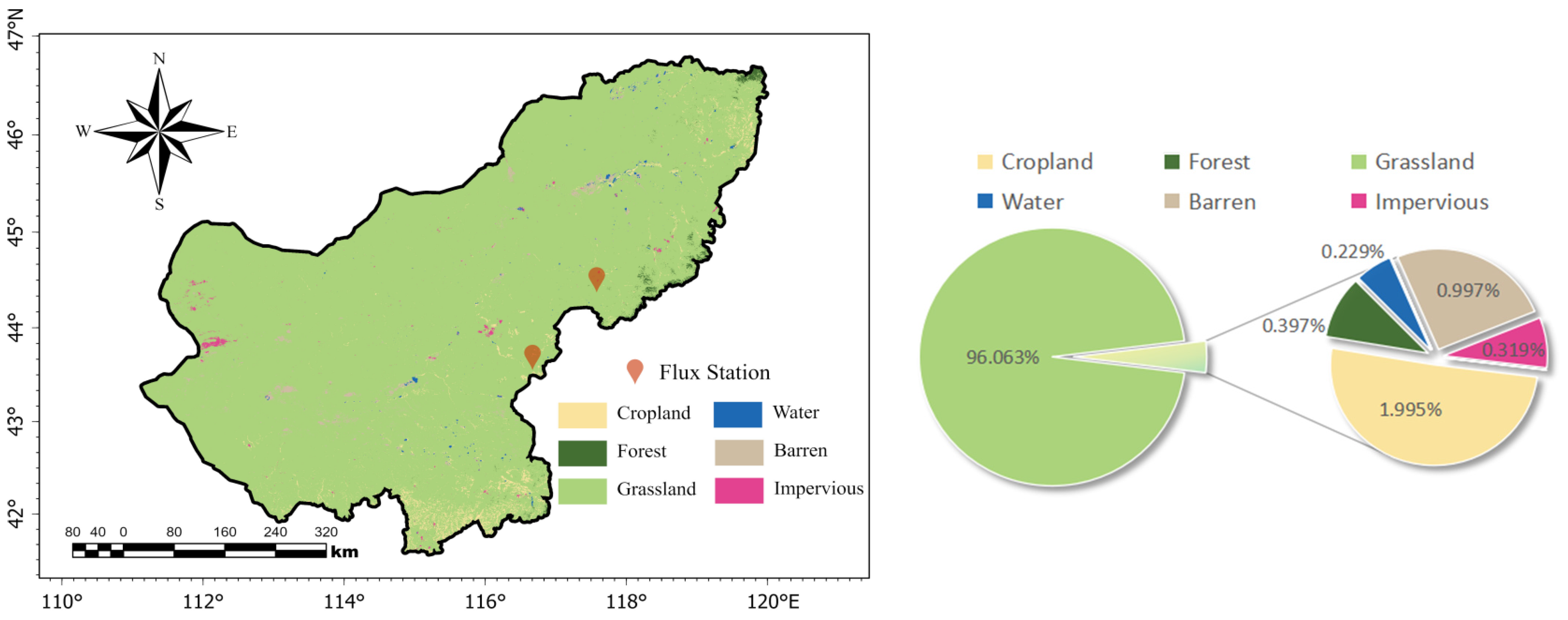
2.1. Overview of the Study Area

Xilin Gol League is located in the central part of the Inner Mongolia Autonomous Region, between 111°03′–120°00′ E and 41°35′–46°46′ N. It covers an area of approximately 203,000 km² with a population of 965,000. The league administratively comprises 9 banners, 1 county, and 2 cities. The average elevation is 1058 m. The eastern and southern parts are characterized by low hills with interspersed basins. The western and northern parts have flat terrain with a sporadic distribution of low hills and volcanic plateaus. The ecosystem structure of Xilin Gol League is simple, primarily composed of herbaceous plants, a small number of shrubs, and wildlife, making it a typical grassland ecosystem. The region experiences a semi-arid continental climate characterized by scarce precipitation, frequent sandstorms, and cold, variable weather conditions. The annual average precipitation is 295 mm, mainly concentrated from July to September. The annual average temperature ranges from 0 to 3 °C, with an annual temperature range of 35–42 °C and a daily temperature range averaging 12–16 °C. The annual total sunshine hours range from 2800 to 3200 h, with a sunshine rate of 64–73%.

Xilin Gol League boasts vast expanses of flat grasslands and a low population density, making it an ideal location for research on grassland evapotranspiration inversion. Due to the scarcity and low accuracy of evapotranspiration data in this region, conducting in-depth studies not only helps fill data gaps but also provides an important research platform for understanding the eco-hydrological processes in semi-arid areas. Given the distribution of precipitation and the growth characteristics of herbaceous plants in the study area, this study selected the period from July to September 2015 as the research timeframe.

2.2. The Selection of Study Blocks

The boundaries between different land use types serve as intuitive criteria for assessing the quality of fused images. However, from the remote sensing image, there is no obvious marker of grassland, and the image boundary is fuzzy and difficult to distinguish after direct image fusion. In order to explore the fusion effect of OL-SS model, it is necessary to select regions with distinct boundaries of different land use combinations for image fusion research and accuracy evaluation. The land use data were raster data with a spatial resolution of 30 m for the year 2015, derived from the 1990–2019 China 30 m annual land cover and land use change dataset (CLCD) produced by the Geospatial Earth Engine team at Wuhan University, led by Huang Xin and Li Jiayi [19]. The original data included nine land use types: cropland, forest, shrub, grassland, water, snow/ice, barren, impervious, wetland. The coordinate system was transformed to WGS-84 World Mercator and the study area was clipped accordingly. Statistical analysis revealed that wetlands and snow/ice occupied a very small area within the study area (0.001% and 0.002%, respectively), and there was no distribution of shrubland. Therefore, these three land use types were omitted in subsequent research. The remaining six land use types were selected for classification, and the distribution of land use types in the study area for the year 2015 is shown in Figure 1.

This study selected common land use combinations in the study area, with sample locations depicted in Figure 2, focusing on water bodies and their surrounding areas (a and d), desert grasslands (b and c), extensive grasslands (e and g), and urban areas with surrounding farmland (f and h). Each type was represented by two square areas of approximately 24 km in side length. It is noteworthy that the flux tower data (1 July 2015~30 September 2015) used in this study were located within two of the grassland sample sites. The datasets from these two flux stations are provided by the National Ecosystem Science Data Center, National Science and Technology Infrastructure of China (http://www.nesdc.org.cn).

The dataset for the e point comes from Xinbaolige Village, Haoletu Gaole Town, Xiwuzhumuqin Banner, Xilin Gol League, Inner Mongolia (44°22′00″ N, 117°34′48″ E) [20]. This dataset includes meteorological and environmental data (such as annual precipitation, temperature, soil moisture, soil temperature, etc.) as well as ecosystem carbon–water flux data (including ecosystem gross primary productivity, ecosystem respiration, ecosystem net carbon exchange, evapotranspiration, carbon use efficiency, and water use efficiency, etc.). Among these, the evapotranspiration data for the e point control group (no treatment) can be regarded as the natural evapotranspiration of the local grassland. The measurement of evapotranspiration is conducted using transparent assimilation chambers, which allow light to pass through, simulating natural light conditions, thereby enabling the measurement of gas exchange within the chambers. The assimilation chambers are connected to an LI-840 infrared gas analyzer (LI-COR Inc., Lincoln, NE, USA) and a gas pump (LI-COR Inc.). The gas pump extracts gas from the assimilation chambers and delivers it to the gas analyzer. Data are collected and stored at fixed intervals using a computer connected to the gas analyzer and the LI-840A software v. 2.1.

The dataset for the g point is sourced from the Baiyin Xile Ranch in Xilinhot, Xilin Gol League, Inner Mongolia Autonomous Region (43°33′16″ N, 116°40′17″ E) [21]. This dataset includes 30 min scale carbon and water flux data (net ecosystem carbon exchange, latent heat flux, and sensible heat flux) and meteorological elements (total radiation, net radiation, soil heat flux, photosynthetically active radiation, air temperature, air relative humidity, precipitation, soil temperature, soil moisture, wind speed, wind direction, friction wind speed, and air pressure). The flux data observed by the eddy covariance system primarily come from the net radiation sensor (CNR1, Kipp & Zonen, Delft, The Netherlands), photosynthetically active radiation sensor (LI-190SB, LICOR, Lincoln, United States), and soil heat flux sensor (HFT-3, SCI, Kyoto, Japan). The eddy covariance system can measure the covariance of vertical wind speed and water vapor concentration, thereby calculating evapotranspiration. By integrating auxiliary data such as net radiation and soil heat flux, the system is capable of providing high-precision evapotranspiration measurement results. The meteorological data measurement frequency is 1 min, and the data are recorded and stored as 30 min averages using a CR23X data logger (CSI). After removing outliers in the flux data based on the g point meteorological data, the filtered flux data are used to calculate the evapotranspiration at the site.

3. Data and Methods

The OL-SS model developed in this study is a high-efficiency grassland evapotranspiration estimation model based in the Google Earth Engine (GEE). This model leverages the fundamental principles of the OL-STARFM to rapidly fuse temporal and spatial images, generating 30 m resolution imagery for the study area. The extracted image bands are then integrated into an enhanced Surface Energy Balance System (SEBS) model tailored for grassland regions, utilizing relevant parameters from the Hourly ERA5-Land dataset for evapotranspiration calculations. Given that the initial evapotranspiration result represents instantaneous values, it is necessary to calculate the daily evaporation ratio using the ERA5-Land Daily dataset. Subsequently, instantaneous evapotranspiration is scaled up to represent daily evapotranspiration using the constant evaporation ratio method. It is noteworthy here that the constant evaporation ratio method was adopted in this model due to its advantage of lower data requirements compared to other methods. For example, the Energy Balance Method requires high-temporal-resolution energy balance data, and the Sine Curve Method requires solar radiation data and instantaneous evapotranspiration values to fit a sine curve. The detailed workflow of the model is illustrated in Figure 3.

3.1. Selection and Application of Datasets

This study utilized the Google Earth Engine (GEE) platform (https://earthengine.google.com/) to construct the OL-SS model, which leverages multisource remote sensing data. To investigate the accuracy of the OL-SS model and its influencing factors, this study designed a comprehensive experimental procedure. Monthly, fine and coarse images for July to September were selected for various study areas. Three prediction experiments were conducted: (1) predicting August images using July images as the base temporal phase; (2) predicting September images using August images as the base temporal phase; (3) predicting September images using July images as the base temporal phase. Base temporal phase images were inputted into the OL-SS model to generate high-resolution fused images of the predicted temporal phases and their daily evapotranspiration.

3.1.1. Datasets for Image Fusion

Landsat 8 Operational Land Imager (OLI) surface reflectance products and Moderate Resolution Imaging Spectroradiometer (MODIS) surface reflectance products were, respectively, employed as the high-resolution and coarse-resolution images required for OL-SS (

Table 1. Description of the datasets available on the GEE platform used in the data fusion part of OL-SS.

Product	GEE ID	Bands	Scale	Offset	Time Coverage	Resolution
LANDSAT 8 OLI/TIRS	LANDSAT/LC08/C02/T1_L2	SR_B2	0.0000275	−0.2	2013-03-18T15:58:14–Present	30 m
		SR_B3
		SR_B4
		SR_B5
		SR_B6
		SR_B7
		ST_EMIS	0.0001	-
		QA_PIXEL	-	-
MCD43A4 V6.1 NBAR product	MODIS/061/MCD43A4	Nadir_Reflectance_Band2	0.0001	0	2000-02-24T00:00:00–Present	500 m
		Nadir_Reflectance_Band3
		Nadir_Reflectance_Band4
		Nadir_Reflectance_Band5
		Nadir_Reflectance_Band6
		Nadir_Reflectance_Band7

).

Landsat 8 surface reflectance products use the LANDSAT/LC08/C02/T1_L2 dataset, which includes images processed through atmospheric and surface temperature orthorectification, suitable directly as fine images for image fusion. The WRS (World Reference System) used by Landsat satellites is a global referencing system that forms a fixed ground reference grid based on the repetitive characteristics of the satellite’s ground track and the imaging characteristics of the satellite’s nadir point. This grid aligns closely with the imaging areas of Landsat satellite data, allowing users to easily locate and query specific areas within the images. The WRS2 system for Landsat 8 imagery provides standard orbit number information and uses PATH and ROW for identification. In GEE, users can directly access the corresponding images by specifying the target image’s time, PATH, and ROW (

Table 2. Landsat time selected for each site.

SITE	a	b	c	d	e	f	g	h
PATH	28	28	30	30	29	29	30	31
ROW	124	124	126	125	124	124	124	124
July Date	7.12	7.12	7.10 *	7.19 *	7.12	7.12	7.12	7.12
August Date	8.13	8.13	8.11	8.04 *	8.13	8.13	8.13	8.13
September Date	9.14	9.14	9.12	9.21	9.14	9.14	9.14	9.14

Note: * represents poor image quality.

).

The MCD43A4 Version 6.1 Minimum Bidirectional Reflectance Distribution Function (BRDF)-Adjusted Reflectance (NBAR) dataset images were selected as the coarse images for image fusion. This dataset represents the most representative pixels from the Terra and Aqua MODIS data within a 16-day retrieval cycle at 500 m resolution, generated daily.

However, the accuracy of fine images directly impacts the final fusion results; if there are large areas of clouds in the images, both evapotranspiration calculation and image fusion will still be significantly affected. Therefore, when selecting monthly images from July to September in the study area, priority was given to images with minimal cloud cover. Visual observation of cloud cover through false-color synthesis indicated that most images in the study area had minimal cloud cover, though a few unavoidably were affected (* noted in the statistics). As shown in Table 2, the number and quality of the filtered images generally meet the research requirements.

Using the GEE platform, the selected images are fused. When performing projection transformation operations on coarse images in GEE, a default nearest-neighbor interpolation method is used for resampling, resulting in new layers. The final fusion results can be exported in GeoTIFF format. Due to the high latitude of the study area, large-area images with boundary projections close to conformal projections in the WGS-84 World Mercator coordinate system (EPSG:3395) were employed.

3.1.2. Datasets for Evapotranspiration Calculation

ERA5-Land is a surface reanalysis data product released by the European Centre for Medium-Range Weather Forecasts (ECMWF), developed based on ECMWF’s advanced reanalysis system, ERA5. As a global meteorological reanalysis dataset, it has a horizontal resolution of 0.25 degrees and a vertical resolution of 137 vertical levels, providing continuous spatiotemporal observations of the atmosphere, surface, and ocean conditions from 1979 to the present. The ERA5-Land Hourly and ERA5-Land Daily datasets are selected as input parameters for the evapotranspiration calculation part of the OL-SS model (

Table 3. Description of the datasets available on the GEE platform used in the evapotranspiration calculation part of OL-SS.

Product	GEE ID	Bands	Scale	Offset	Time Coverage	Resolution
ERA5-Land Hourly	ECMWF/ERA5_LAND/HOURLY	skin_temperature	1	0	1950-01-01T01:00:00–Present	0.1°
		surface_solar_radiation_downwards_hourly
		surface_thermal_radiation_downwards_hourly
		temperature_2m
		u_component_of_wind_10m
		v_component_of_wind_10m
ERA5-Land Daily	ECMWF/ERA5_LAND/DAILY_AGGR	surface_net_solar_radiation_sum	1	0	1950-01-02T00:00:00–Present	0.1°
		surface_net_thermal_radiation_sum

). The main operations include:

Based on the basic principles of the SEBS model, meteorological parameters are extracted by importing the ECMWF/ERA5_LAND/HOURLY dataset on the GEE platform. These parameters are then combined with the fused imagery to select bands required by the model for calculating instantaneous evapotranspiration. Next, the ECMWF/ERA5_LAND/DAILY_AGGR dataset is imported to calculate the evaporation ratio, and the constant evaporation ratio method is applied to determine the daily evapotranspiration for the study area. However, the ERA5_LAND data have limitations in terms of spatial resolution, accuracy of meteorological elements, and terrain effects, which may not fully capture local microclimate variations, thereby introducing some uncertainty into the final results. Nevertheless, the ERA5_LAND data offer advantages such as long-term coverage, high temporal resolution, and a good representation of land surface hydrological processes, making it an ideal data source for input into evapotranspiration models.

3.2. Model Referenced for OL-SS Construction

3.2.1. OL-STARFM

One difference between the OL processing strategy and traditional weighted function-based methods lies in the modification of assumptions. OL processing assumes pixels within the same segmentation object share similar spectral characteristics and change patterns, maintaining feature shape consistency during fusion. Based on these assumptions, the OL strategy employs a multi-resolution segmentation algorithm to partition the overlaid fine images into regions that change uniformly over time series rather than uniformly over a base image. This makes segmented objects the fundamental analysis units instead of pixels. Guo et al. extensively discussed the principles of the OL processing strategy in their work; for further details, refer to reference [18]. This study employs the OL-STARFM method for Landsat 8 and MODIS data fusion, computing the difference between MODIS images at two time periods, taking the median within each segmentation block, and adding it to the Landsat image.

The original STARFM can be represented as:

$${\widehat{F}}_p\left(x,y,B\right)=\sum _{b=1}^M\sum _{i=1}^N{W}_b(x_i,y_i,B)·\left[F_b\right(x,y,B)+C_p(x_i,y_i,B)-C_b(x_i,y_i,B\left)\right],$$

(1)

where F is the fine pixel value, p is the prediction phase, (x, y) is the location of the target fine pixel, B is for band index, M is the number of auxiliary image pairs, N is the number of spectrally similar neighboring pixels, W is the weighting function, b is the base phase, and ($x_i,y_i$) is the location of its first spectrally similar neighboring pixel.

The coarse image is resampled to a finer resolution by the nearest neighbor interpolation method, and then the fine image segmentation is assisted. The principle of the OL processing version of STARFM (OL-STARFM) can be expressed as:

$${\widehat{F}}_p^{\prime }\left(s,B\right)=F_b(s,B)+M[C_p(s,B)-C_b(s,B)],$$

(2)

where M[·] takes the median of all pixel values within the object.

OL-STARFM uses the median instead of the mean to mitigate the impact of low-quality pixels across the entire segmentation object. To minimize potential uncertainties associated with this strategy, a residual compensation (RC) step has been introduced. This step involves pixel-level computations without merging similar adjacent information, thereby enhancing preliminary fusion results while requiring less computation time:

$${\widehat{F}}_p={\widehat{F}}_p^{\prime }+R,$$

(3)

where the residual R is the difference in temporal changes between the coarse and fine images.

To enhance the image quality, bicubic interpolation is employed to remove blocky pseudo-shadows in residuals, resulting in smoother and more continuous pixel values in the resultant image.

It is noteworthy that the “LANDSAT/LC08/C01/T1_SR” dataset used in the original study has been replaced by “LANDSAT/LC08/C02/T1_L2”. The algorithm used for processing “LANDSAT/LC08/C02/T1_L2” images is the Land Surface Reflectance Code (LaSRC, version 1.5.0). The scale factor and offset used by this algorithm have changed compared to earlier versions and are now different from the conversion formula used for the “MODIS/061/MCD43A4” dataset. Therefore, in this study, data extracted from “LANDSAT/LC08/C02/T1_L2” are adjusted using conversion factors consistent with those of “MODIS/061/MCD43A4”, and the fused results are calculated uniformly according to the conversion formula of “MODIS/061/MCD43A4”.

3.2.2. SEBS Model

The SEBS model, based on the concept of surface energy balance, considers the exchange of energy between the land surface and the atmosphere. The surface energy balance is typically expressed as:

$$R_n=G_0+H+\lambda E,$$

(4)

where $R_n$ is the net radiation flux at the land surface (W/m²); $G_0$ is the soil heat flux (W/m²); $\lambda E$ is the latent heat flux, where $\lambda$ is the latent heat of water vaporization (J/kg), and $E$ is the evapotranspiration; and $H$ is the sensible heat flux (W/m²).

By using various parameters derived from remote sensing data to calculate different flux components in the SEBS model, evapotranspiration can be estimated.

(1) Net radiation at the land surface:

$$R_n=(1-\alpha )·R_{swd}+\epsilon ·R_{lwd}-\epsilon ·\sigma ·T_s^4,$$

(5)

where $\alpha$ is the surface albedo; $R_{swd}$ is the downward solar radiation; $R_{lwd}$ is the downward longwave radiation; $\epsilon$ is the emissivity; and $\sigma$ is the Stefan–Boltzmann constant, with a value of 5.6697 × 10⁻⁸ W·m⁻²·k⁻⁴; $T_s$ is the surface temperature (K). The estimation method for surface albedo follows the research by Ke et al. [22].

(2) Soil heat flux:

$$G_0=R_n·[{\Gamma }_c+(1-f_c)·({\Gamma }_s-{\Gamma }_c\left)\right],$$

(6)

where ${\Gamma }_c$ is the fraction of net radiation allocated to soil heat flux under full vegetation cover (${\Gamma }_c$ = 0.05); ${\Gamma }_s$ is the fraction of net radiation allocated to soil heat flux over bare soil (${\Gamma }_s$ = 0.315) [23]; is the vegetation cover fraction, calculated using the Normalized Difference Vegetation Index (NDVI):

$$f_c={\displaystyle \frac{NDVI-{NDVI}_{min}}{{NDVI}_{max}-{NDVI}_{min}}},$$

(7)

(3) Sensible heat flux:

$$H={\displaystyle \frac{\rho C_p(T_s-T_a)}{{\gamma }_a}},$$

(8)

where $\rho$ is the air density, with a value of 1.29 kg/m³; $C_p$ is the specific heat capacity of air at constant pressure, with a value of 1005 J·kg⁻¹·K⁻¹; $T_a$ is the temperature at the reference height (K); and ${\gamma }_a$ is the aerodynamic resistance (s/m).

Aerodynamic resistance often depends on wind speed and roughness length at the reference height. In this study, calculations are based on formulas derived by the Food and Agriculture Organization (FAO) of the United Nations using temperature and humidity data at 2 m height. To ensure uniformity and standardization of the calculation formula, FAO provides a new definition of reference crop evapotranspiration based on the Penman–Monteith equation, as follows: reference crop evapotranspiration is the hypothetical evapotranspiration rate of a reference crop canopy. Assuming a crop height of 0.12 m, fixed leaf surface resistance of 70 s/m, and an albedo of 0.23, it closely resembles the evapotranspiration from a well-watered, extensively vegetated grass surface with uniform growth and complete shading [24].

$${\gamma }_a={\displaystyle \frac{208}{v_2}},$$

(9)

where $v_2$ is the wind speed at 2 m height.

Due to this study, wind speeds at 10 m from the ERA5 dataset, accessed via GEE, are converted to wind speeds at 2 m using a power law formula:

$$v_2=v_1{\left({\displaystyle \frac{z_2}{z_1}}\right)}^{ws},$$

(10)

where $ws$ is the wind shear exponent ($ws$ = 0.143); $z_1$ is the known height (m); $z_2$ is the height where the wind speed is adjusted (m); $v_1$ is the wind speed at height (m/s); and $v_2$ is the wind speed at height (m/s). Due to the absence of measured wind speeds at different heights, a power law fit is applied here, assuming a constant power law exponent of 0.143.

(4) Evaporation ratio

Evapotranspiration, calculated based on the energy balance equation, represents instantaneous values at the time of satellite overpass. This study employs the constant evaporation ratio method [25] to extrapolate daily evapotranspiration from instantaneous evapotranspiration:

$$EF={\displaystyle \frac{\lambda E}{R_n-G_0}},$$

(11)

$${ET}_{24}=8.64\times {10}^7\times EF\times {\displaystyle \frac{R_{n24}-G_{024}}{\lambda {\rho }_w}},$$

(12)

where ${ET}_{24}$ is the daily actual evapotranspiration (mm); $EF$ is the evaporation ratio; $R_{n24}$ is the daily net radiation flux (W/m²); $G_{024}$ is the daily soil heat flux (W/m²); and ${\rho }_w$ is the density of water, with a value of 1000 kg·m⁻³. In this equation, the daily soil heat flux is often neglected. $\lambda$ represents the latent heat of vaporization of water (J/kg), and its calculation formula is:

$$\lambda =(2.501-2.361\times {10}^{-3}(T_a-273.15\left)\right)\times {10}^6,$$

(13)

4. Results

To validate whether the images generated by the newly proposed grassland evapotranspiration spatiotemporal fusion model (OL-SS) can preserve structural information and significantly improve the efficiency of grassland evapotranspiration calculations based on spatiotemporal fusion, RMSE (Root Mean Squared Error), AAD (Average Absolute Deviation), and RMSPE (Root Mean Squared Percentage Error) are used as accuracy evaluation metrics for the fusion results. RMSE is the square root of the average of the squared differences between predicted values and actual values, mainly focusing on the overall amount of error and the impact of large errors. AAD is the average of the absolute values of all prediction errors, emphasizing the average error level, particularly when the error distribution is uniform. RMSPE is the square root of the average of the squared percentage differences between prediction errors and actual values, focusing on evaluating the relative accuracy of predictions, and is used to compare model performance across predictions of different scales.

The three accuracy assessment metrics mentioned above are commonly used to evaluate image fusion models. If all these metrics are within 10%, they are generally considered to indicate good model performance. These accuracy metrics allow for a comprehensive evaluation of the fusion results’ precision from different perspectives, providing more complete feedback on the model’s performance. To present the fusion accuracy more intuitively and conveniently, a segment of code has been added in the OL-SS model to directly calculate these metrics in GEE.

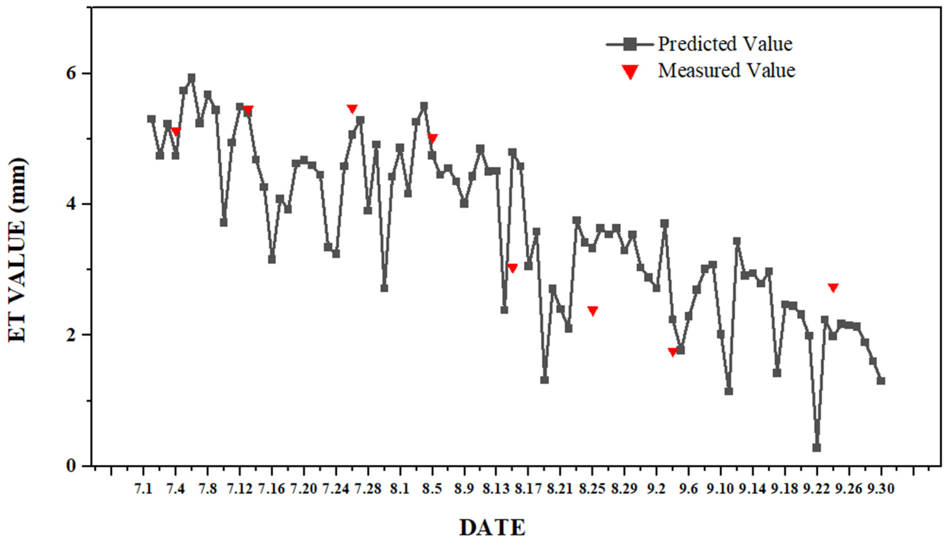
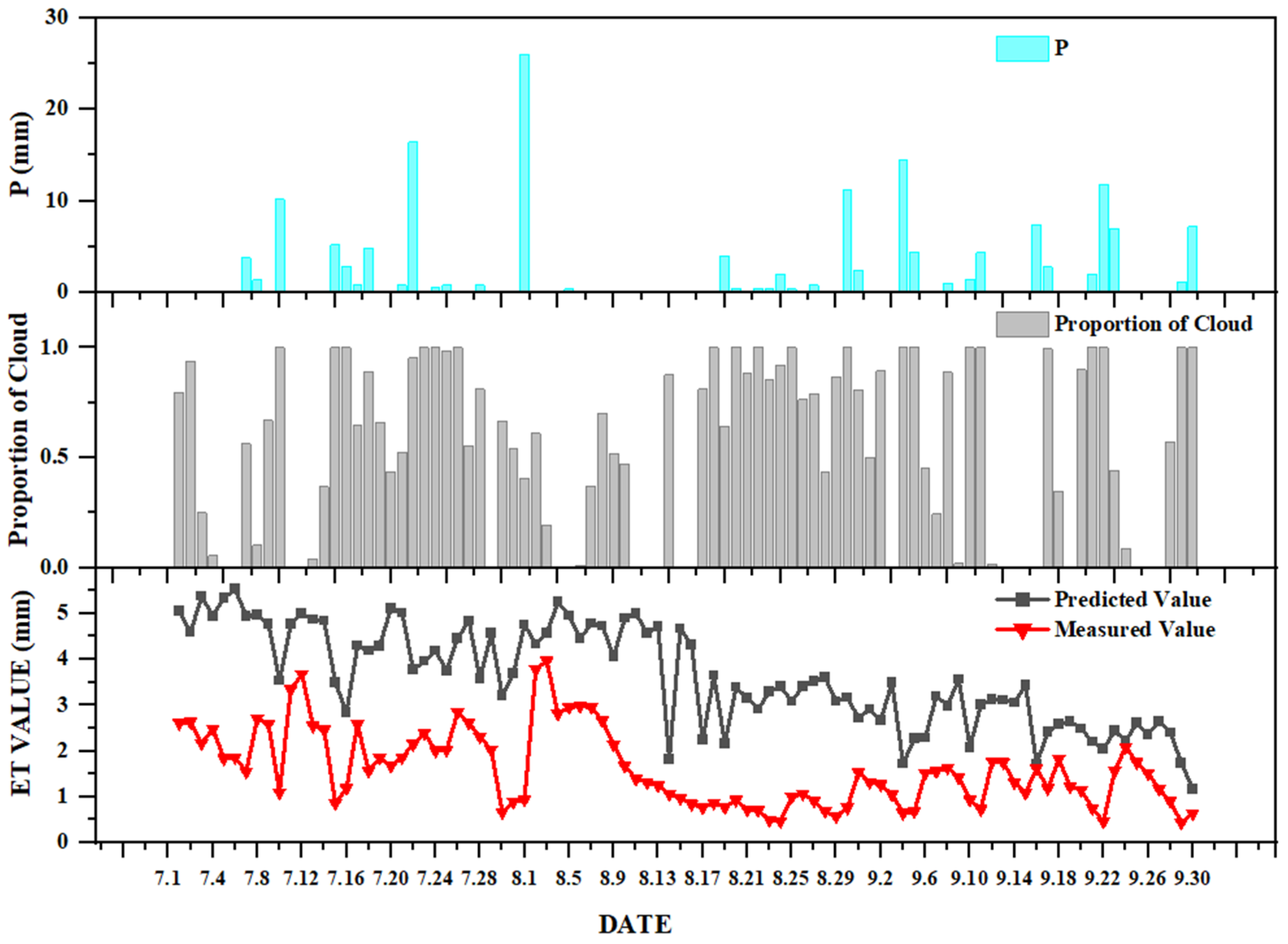
4.1. Fusion Result Evaluation

Fusion images for August and September calculated by the OL-SS model are compared with corresponding fine images (

Table 4. Fusion accuracy statistics.

Sites	Time	Indexes
		RMSE	AAD	RMSPE
a	7→8	0.0363	0.0252	0.2443
	8→9	0.0367	0.0260	0.2340
	7→9	0.0347	0.0221	0.2501
b	7→8	0.0295	0.0204	0.1466
	8→9	0.0278	0.0187	0.1495
	7→9	0.0351	0.0218	0.1934
c	7→8	0.1168	0.0909	0.4107
	8→9	0.0377	0.0221	0.1340
	7→9	0.1272	0.0975	0.4815
d	7→8	0.1427	0.0819	0.5945
	8→9	0.1017	0.0724	0.5127
	7→9	0.1600	0.1127	0.6962
e	7→8	0.0141	0.0099	0.0988
	8→9	0.0174	0.0124	0.1113
	7→9	0.0212	0.0148	0.1409
f	7→8	0.0549	0.0374	0.3145
	8→9	0.0530	0.0363	0.3429
	7→9	0.0326	0.0188	0.1966
g	7→8	0.0188	0.0136	0.1157
	8→9	0.0322	0.0214	0.2023
	7→9	0.0197	0.0135	0.1231
h	7→8	0.0248	0.0155	0.1701
	8→9	0.0258	0.0156	0.1801
	7→9	0.0296	0.0185	0.2163

). Overall, the fusion results are satisfactory, though a few fusion results are less ideal.

In combination with Table 2, the fusion images with relatively poor prediction results are selected from high-resolution images that completely overlap with low-quality fine-resolution images. Therefore, the precision of the fine image used for homogeneous cutting, relative to the predicted time span, is a direct factor affecting the final fusion effect.

4.2. Fusion Result Verification

The evapotranspiration data at the e point were measured during good weather conditions and clear mornings (8:00–11:00 a.m.), which helps ensure the accuracy of the actual evapotranspiration measurements to some extent.

The daily evapotranspiration data curve generated by the OL-SS model for July to September 2015 was compared with the actual evapotranspiration data measured at fixed intervals from the e point. As shown in Figure 4, the OL-SS model’s predictions at the e point closely match the observed evapotranspiration data, with the predicted values accurately reflecting the evapotranspiration trend.

The evapotranspiration data at the g point were derived from flux calculations. It was necessary to remove outliers from the data before fitting the daily evapotranspiration data generated by the OL-SS model. This is because the local, intense weather variations in the grassland during the summer present significant challenges to evapotranspiration observations. The study period from July to September coincides with the season of frequent precipitation and higher cloud cover in the grassland, which can reduce the accuracy of flux observations. The poor energy closure of the flux data at the g point during the study period further supports this point [22]. As a result, the evapotranspiration data calculated from the g point flux measurements may not fit well with the OL-SS model’s results under unfavorable weather conditions (Figure 5).

From the researchers’ perspective, calculating daily evapotranspiration using latent heat flux at half-hour intervals is significantly influenced by environmental factors, leading to discrepancies with remote sensing-derived evapotranspiration results. Therefore, in this study, data from the g point with minimal cloud cover and no rainfall during satellite observation periods were selected, and instantaneous flux at 11 a.m. was extrapolated to a daily scale. This yielded several high-confidence daily evapotranspiration data points, which were then combined with the daily evapotranspiration data from the e point as the observed evapotranspiration data for this study. The fitting results of the observed data are shown in Figure 6. From the figure, it can be seen that the OL-SS model provides a good fit for the daily evapotranspiration data.

5. Discussion

In this study, we successfully developed an efficient grassland evapotranspiration spatiotemporal fusion model based on the Google Earth Engine (GEE), aimed at integrating image spatiotemporal fusion and high-resolution evapotranspiration retrieval in grassland areas. Our results demonstrate that the model excels in both accuracy and efficiency in image fusion and evapotranspiration retrieval. It significantly improves identification accuracy compared to traditional evapotranspiration retrieval methods. Particularly in terms of efficiency in retrieval, we leveraged advanced multisource remote sensing image access through the GEE, effectively enhancing computational performance. The image fusion results align with previous research, confirming the potential and advantages of the OL processing strategy in achieving spatiotemporal fusion of images [18]. Moreover, the process of evapotranspiration retrieval typically involves parameters such as solar radiation and net radiation, which are hindered by the high costs associated with necessary measuring equipment [26,27], whereas the OL-SS model utilizes the ERA5 dataset to access and compute these parameters, thereby overcoming, to some extent, the challenges associated with acquiring such parameters. In addition, models such as the OL-STARFM, which are currently being used for spatiotemporal fusion, have not been updated for a long time, and the outdated data sources they rely on make them no longer directly applicable. The OL-SS model constructed in this study improves this by converting the bands of coarse-resolution image data sources to the standards of fine-resolution image bands, resulting in better fusion outcomes.

Despite our model demonstrating excellent performance under experimental conditions, we must also consider several potential limiting factors. Firstly, the quality of high-resolution images is crucial for the model’s prediction accuracy. In this study, the impact of image quality outweighed the influence of the prediction time span on results. For certain grassland areas, frequent summer precipitation and high cloud cover are unavoidable. Although the model employs mean value imputation to fill gaps caused by cloud cover and other factors in the results after masking, the difficulty in obtaining high-quality images may still limit the practical application of the OL-SS model. Similarly, obtaining actual measurement data also presents significant challenges, with over 80% of previous studies involving predictions at fewer than 10 sites, and with approximately 40% focusing solely on one site [28]. Therefore, future research can focus on addressing these challenges by integrating additional satellite datasets (such as Sentinel-2 and PlanetScope) to obtain high-resolution images at different times of the day. This approach can mitigate the impact of low-quality images caused by clouds and enrich observations of instantaneous evapotranspiration values throughout the day, thereby making the results more reasonable. Additionally, acquiring and sharing more ground measurement data, and fitting the model results with actual measurements, can help calibrate the model outputs and enhance the credibility of the model.

However, significant discrepancies were observed between the OL-SS model simulations and the measured evapotranspiration at site g, which may be related to multiple factors. For instance, measurement errors from the flux tower, sensor calibration biases in the eddy covariance method, or high-frequency signal loss could lead to energy closure issues, ultimately affecting the actual measurement results. Additionally, parameterization of boundary layer turbulence and surface roughness in the model might introduce modeling deviations. Such deviations could be amplified under conditions of intense intraday weather variations, thereby impacting the final model outputs. Additionally, while our study focused on evapotranspiration retrieval in the Xilingol Grassland, significant differences may exist between different geographical environments, potentially affecting the universality and adaptability of the model. Therefore, addressing the research needs of different ecosystems and species populations remains a key focus of future work, to validate and optimize the widespread applicability and practicality of our model.

In summary, the advantages of the model developed in this study are twofold: First, the model has a certain advantage in terms of temporal scale, as it can meet the requirements for daily evapotranspiration (ET) calculations, whereas other ET datasets typically have lower temporal resolutions, such as monthly (e.g., OpenET’s geeSEBAL and eeMETRIC) or every eight days (geeSEBAL-MODIS). Compared to other models like geeSEBAL that also support daily ET calculations, the OL-SS model utilizes data for ET calculation that has undergone spatiotemporal fusion, resulting in superior temporal scale quality. Therefore, the ET results derived from the OL-SS model are theoretically more accurate. Second, the model is theoretically more stable in evapotranspiration calculation. The OL-SS model uses an aerodynamic resistance calculation method suitable for grassland areas to compute sensible heat flux, minimizing the sensitivity and uncertainty issues related to the selection of hot and cold end points. Therefore, theoretically, the OL-SS model has better stability in evapotranspiration calculations for grassland areas.

In conclusion, while our study demonstrated the potential of the OL-SS model in efficient spatiotemporal fusion of evapotranspiration in grasslands, challenges still need to be addressed for its wider dissemination and practical application. By continuing to improve data quality, model architecture, and adaptability to application scenarios, we can further enhance the reliability and practicality of the model, better supporting practical needs in evapotranspiration monitoring and water resource management.

6. Conclusions

Spatial-temporal fusion of remote sensing images for evapotranspiration estimation is a cost-effective approach for large grassland areas where observational data are limited. However, the low efficiency of spatial-temporal fusion models and the challenges in obtaining meteorological parameters for evapotranspiration models severely restrict large-scale and high-precision evapotranspiration observations in grassland regions. To address this issue, this study proposes an evapotranspiration model suitable for large grassland areas based on the OL-STARFM spatial–temporal fusion algorithm and SEBS model.

Leveraging the GEE platform, we developed the OL-SS model using multiple datasets and compared the computed evapotranspiration results with actual observations from two flux towers within Xilingol League. The results indicate an R² of 0.82391 for the OL-SS model. Since the model developed in this study does not require additional ground measurement data as inputs, it enables high spatiotemporal resolution evapotranspiration estimation in large grassland areas with limited data. We aim for this research to contribute to water and energy balance studies in large grassland regions and global water resources management.

The code snapshot of this model is available at the following URL: https://code.earthengine.google.com/a3d6df68bb99877f50bf19598c9a7209.

References

1. Bardgett, R.D.; Bullock, J.M.; Lavorel, S.; Manning, P.; Schaffner, U.; Ostle, N.; Chomel, M.; Durigan, G.; Fry, E.L.; Johnson, D.; et al. Combatting global grassland degradation. Nat. Rev. Earth Environ. 2021, 2, 720–735. [Google Scholar] [CrossRef]
2. Chen, L.D.; Wang, J.P.; Wei, W.; Fu, B.J.; Wu, D.P. Effects of landscape restoration on soil water storage and water use in the Loess Plateau Region, China. For. Ecol. Manag. 2010, 259, 1291–1298. [Google Scholar] [CrossRef]
3. Wang, Y.S.; Zhang, Y.G.; Yu, X.X.; Jia, G.D.; Liu, Z.Q.; Sun, L.B.; Zheng, P.F.; Zhu, X.H. Grassland soil moisture fluctuation and its relationship with evapotranspiration. Ecol. Indic. 2021, 131, 9. [Google Scholar] [CrossRef]
4. Yinglan, A.; Wang, G.Q.; Liu, T.X.; Xue, B.L.; Kuczera, G. Spatial variation of correlations between vertical soil water and evapotranspiration and their controlling factors in a semi-arid region. J. Hydrol. 2019, 574, 53–63. [Google Scholar] [CrossRef]
5. Su, Z. The Surface Energy Balance System (SEBS) for estimation of turbulent heat fluxes. Hydrol. Earth Syst. Sci. 2002, 6, 85. [Google Scholar] [CrossRef]
6. Laipelt, L.; Kayser, R.H.B.; Fleischmann, A.S.; Ruhoff, A.; Bastiaanssen, W.; Erickson, T.A.; Melton, F. Long-term monitoring of evapotranspiration using the SEBAL algorithm and Google Earth Engine cloud computing. ISPRS J. Photogramm. Remote Sens. 2021, 178, 81–96. [Google Scholar] [CrossRef]
7. Nkiaka, E.; Bryant, R.G.; Dembélé, M.; Yonaba, R.; Imuwahen Priscilla, A.; Karambiri, H. Quantifying the effects of climate and environmental changes on evapotranspiration variability in the Sahel. J. Hydrol. 2024, 642, 131874. [Google Scholar] [CrossRef]
8. Mu, Q.Z.; Zhao, M.S.; Running, S.W. Improvements to a MODIS global terrestrial evapotranspiration algorithm. Remote Sens. Environ. 2011, 115, 1781–1800. [Google Scholar] [CrossRef]
9. Senay, G.B.; Bohms, S.; Singh, R.K.; Gowda, P.H.; Velpuri, N.M.; Alemu, H.; Verdin, J.P. Operational Evapotranspiration Mapping Using Remote Sensing and Weather Datasets: A New Parameterization for the SSEB Approach. J. Am. Water Resour. Assoc. 2013, 49, 577–591. [Google Scholar] [CrossRef]
10. Zheng, C.L.; Jia, L.; Hu, G.C. Global land surface evapotranspiration monitoring by ETMonitor model driven by multi-source satellite earth observations. J. Hydrol. 2022, 613, 21. [Google Scholar] [CrossRef]
11. Miralles, D.G.; Holmes, T.R.H.; De Jeu, R.A.M.; Gash, J.H.; Meesters, A.; Dolman, A.J. Global land-surface evaporation estimated from satellite-based observations. Hydrol. Earth Syst. Sci. 2011, 15, 453–469. [Google Scholar] [CrossRef]
12. Liu, M.; Yang, W.; Zhu, X.L.; Chen, J.; Chen, X.H.; Yang, L.Q.; Helmer, E.H. An Improved Flexible Spatiotemporal DAta Fusion (IFSDAF) method for producing high spatiotemporal resolution normalized difference vegetation index time series. Remote Sens. Environ. 2019, 227, 74–89. [Google Scholar] [CrossRef]
13. Belgiu, M.; Stein, A. Spatiotemporal Image Fusion in Remote Sensing. Remote Sens. 2019, 11, 818. [Google Scholar] [CrossRef]
14. Gao, F.; Masek, J.G.; Schwaller, M.R.; Hall, F.G. On the blending of the Landsat and MODIS surface reflectance: Predicting daily Landsat surface reflectance. IEEE Trans. Geosci. Remote Sens. 2006, 44, 2207–2218. [Google Scholar] [CrossRef]
15. Lee, Y.; Terzopoulos, D.; Waters, K. Constructing Physics-Based Facial Models of Individuals. Graph. Interface 1993, 1–8. [Google Scholar]
16. Wang, J.; Huang, B. A Rigorously-Weighted Spatiotemporal Fusion Model with Uncertainty Analysis. Remote Sens. 2017, 9, 990. [Google Scholar] [CrossRef]
17. Wang, Q.M.; Atkinson, P.M. Spatio-temporal fusion for daily Sentinel-2 images. Remote Sens. Environ. 2018, 204, 31–42. [Google Scholar] [CrossRef]
18. Guo, D.Z.; Shi, W.Z.; Zhang, H.; Hao, M. A Flexible Object-Level Processing Strategy to Enhance the Weight Function-Based Spatiotemporal Fusion Method. IEEE Trans. Geosci. Remote Sens. 2022, 60, 11. [Google Scholar] [CrossRef]
19. Yang, J.; Huang, X. The 30 m annual land cover dataset and its dynamics in China from 1990 to 2019. Earth Syst. Sci. Data 2021, 13, 3907–3925. [Google Scholar] [CrossRef]
20. Tan, X.; Zhang, B.; Chen, S. A dataset of observational key parameters in carbon and water fluxes in a semi-arid steppe, Inner Mongolia (2012–2020): Based on a long-term manipulative experiment of precipitation pattern. China Sci. Data 2023, 8, 1–11. [Google Scholar] [CrossRef]
21. You, C.; Wang, Y.; Chen, S. A dataset of carbon and water fluxes of the typical grasslands in Duolun County, Inner Mongolia during 2006–2015. China Sci. Data 2023, 8, 1–11. [Google Scholar] [CrossRef]
22. Ke, Y.H.; Im, J.; Park, S.; Gong, H.L. Downscaling of MODIS One Kilometer Evapotranspiration Using Landsat-8 Data and Machine Learning Approaches. Remote Sens. 2016, 8, 215. [Google Scholar] [CrossRef]
23. Nishida, K.; Nemani, R.R.; Running, S.W.; Glassy, J.M. An operational remote sensing algorithm of land surface evaporation. J. Geophys. Res. Atmos. 2003, 108, 1–14. [Google Scholar] [CrossRef]
24. Allen, R.; Smith, M.; Perrier, A.; Pereira, L.S. An update for the definition of reference evapotranspiration. ICID Bull. 1994, 43, 1–34. [Google Scholar]
25. Shuttleworth, W.; Gurney, R.; Hsu, A.; Ormsby, J. FIFE: The variation in energy partition at surface flux sites. IAHS Publ. 1989, 186, 523–534. [Google Scholar]
26. Guven, A.; Aytek, A.; Yuce, M.I.; Aksoy, H. Genetic programming-based empirical model for daily reference evapotranspiration estimation. Clean–Soil Air Water 2008, 36, 905–912. [Google Scholar] [CrossRef]
27. Shiri, J.; Kişi, Ö.; Landeras, G.; López, J.J.; Nazemi, A.H.; Stuyt, L.C. Daily reference evapotranspiration modeling by using genetic programming approach in the Basque Country (Northern Spain). J. Hydrol. 2012, 414, 302–316. [Google Scholar] [CrossRef]
28. Valipour, M.; Khoshkam, H.; Bateni, S.M.; Jun, C.; Band, S.S. Hybrid machine learning and deep learning models for multi-step-ahead daily reference evapotranspiration forecasting in different climate regions across the contiguous United States. Agric. Water Manag. 2023, 283, 108311. [Google Scholar] [CrossRef]
Figure 1. Land use distribution and its proportion in Xilingol League in 2015.
Water 17 01034 g001
Figure 2. Eight plot locations for four land use combinations. Note: water bodies and their surrounding areas (a,d), desert grasslands (b,c), extensive grasslands (e,g), and urban areas with surrounding farmland (f,h).
Water 17 01034 g002
Figure 3. Workflow adopted by OL-SS model.
Water 17 01034 g003
Figure 4. Predicted values and measured values of evapotranspiration in e.
Water 17 01034 g004
Figure 5. Daily precipitation (P), the proportion of cloud cover calculated based on MODIS MOD09GQ, the predicted values simulated based on OL-SS model (predicted values), and the measured values converted from the latent heat flux recorded at a half-hour interval (measured values) in g from 1 July 2015 to 30 September 2015.
Water 17 01034 g005
Figure 6. The fitting results between the measured values and the predicted values of the OL-SS model.
Water 17 01034 g006