Semi-Automated Extraction and Geomorphic Analysis of Flat Surface Landforms in Large Areas

Abstract

The semi-automated extraction of flat surface landforms was carried out, merging a GIS tools application and a geomorphic analysis. The study focuses on seven areas in southern Italy, characterized by different physical landscapes, using a 5 m resolution digital elevation model (DEM). The GIS application allowed the selection of polygonal areas of flat surfaces from diverse arrays of landforms and was implemented using a filtering process to minimize noises. Subsequently, the mean elevation and mean slope of the detected surfaces were extracted and visualized using scatter plots, which helped in determining the elevation ranges and average slope angles for various flat-floored and terraced surfaces. To enhance the reliability of the results, a detailed geomorphic analysis and field survey were conducted to differentiate between fluvial and marine flat surfaces across different physical landscapes. This comprehensive approach included statistical analyses and comparisons with the existing literature to validate the identified flat surfaces, ensuring the accuracy and reliability of the semi-automated extraction procedure. The integration of GIS technology with field investigations not only streamlines the detection of flat landforms but also contributes to a deeper understanding of their geomorphic characteristics, ultimately enhancing geomorphic analysis efficiency.

1. Introduction

Plain and low-angle landscapes, characterized by small or no differences in topographic elevation, are known in geomorphology as flat surfaces and correspond to depositional and/or erosional top surfaces [1,2]. Flat surfaces can be found in several different geomorphic systems, such as glacial, fluvial, aeolian, and marine. A significant distribution of these landforms is found in fluvial and marine landscapes, which are among the common earth’s physical landscapes. Recognizing flat surface landforms provides useful information on a region’s morphological evolution, on an area’s potential hazard, and on a territory’s urban development. Flat surfaces in the fluvial system are represented by floodplains and terraces. The first are flat areas of the alluvial system stretching from the channel stream to the base of the valley walls and over which channel water flows at times of high discharge [1,2,3,4,5,6]. Fluvial terraces are remnants of a former floodplain surface preserved at higher elevation and are underlain by alluvial deposits resting on the flank valley, which occurs in a wide range of climatic and tectonic settings [5,6,7]. Flat surfaces in the marine system are represented by coastal plains and marine terraces. The coastal plain is formed by a plain flat surface and by dune landforms distributed from the beach to inland areas [2,8]. Marine terraces are elevated wave-cut benches, marking former high sea levels and produced by the falling of sea levels along a coastline [1,2,9]. In transitional zones, where both alluvial and coastal plains co-exist, the fluvial-mouth landforms merge with the coastal plain ones. Fluvial and marine landforms typically form topographically flat or low-angle slope surfaces distributed over large or small areas. In the past, the flat landform extraction was usually realized by handmade methods, aerial photos, and/or contour maps integrated with field surveys. In the last decades, their recognition was made possible thanks to the availability of topographic datasets provided by digital elevation models (DEMs) [10,11]. Many methods have implemented geographical information system (GIS) routines for the automated or semi-automated detection of flat surfaces. Knowledge on process-based surface relationships has allowed many authors to extract specific landform types based on morphological features due to different geological and physical landscapes [4,9,10,11,12,13,14,15,16,17,18,19,20,21,22,23,24,25,26]. The robustness of results obtained from different DEMs resolution and GIS applications was analyzed using semi-automated extraction and classification of landforms [27]. Remote mapping approaches based on multi-source and multi-sensor applications were recently implemented in the detection of landforms and processes furnishing multi-scale and multi-temporal modeling in their cartographic representation [28]. A more complete review of the most recent landforms classification methods was listed in recent papers [29,30]. The first authors [29] analyzed statistical data on the current knowledge of landform classification, identifying more used methodologies, whereas the second authors [30] addressed the research on the geomorphology-oriented digital terrain analysis.

The objective of this study was to identify and analyze the spatial distribution of flat surface landforms within a complex physical landscape such as that of southern Italy and specifically in large regions where both fluvial and marine flat surfaces are present. This was achieved by integrating a semi-automated GIS extraction and classification method and a geomorphic analysis of landforms. The flat landforms of seven selected areas were extracted using a toolbox in ArcGis 10.7 (

Table 1. Spatial extent and centroid coordinates of each studied area.

Site	Area (Km2)	Centroid Coordinates
1	25	40°44′13.60″ N–16° 9′1.92″ E
2	25	40°17′4.74″ N–15°55′46.71″ E
3	36	40°16′8.12″ N–16°16′32.25″ E
4	25	40°9′2.35″ N–16°20′40.53″ E
5	6	40°8′15.11″ N–16°24′50.05″ E
6A	80	40°9′11.59″ N–16°36′17.63″ E
6B	7.5	40°7′57.02″ N–16°34′53.57″ E
7A	100	40°20′2.91″ N–16°42′31.56″ E
7B	6	40°19′6.16″ N–16°39′49.09″ E

). To discriminate between fluvial and marine flat surfaces, data gathered from geomorphic analyses and field surveys were employed. The study also categorized the flat landforms within both the fluvial and marine systems into (i) present-day features (such as floodplains and coastal plains) and (ii) ancient ones (including terraced surfaces). Furthermore, the effectiveness of the semi-automated extraction process was validated by comparing the results with mappings from field surveys and previously published research. This comprehensive approach enhances the understanding of landform distribution in this diverse landscape, providing a reliable application for future geomorphological studies.

This study aimed to analyze the spatial distribution of flat surface landforms in southern Italy, focusing on regions with both fluvial and marine flat surfaces. Using a semi-automated GIS extraction method and geomorphic analysis, flat landforms from seven selected areas were identified with ArcGIS 10.7. Additionally, data from field surveys helped distinguish between fluvial and marine surfaces. Flat landforms were categorized into present-day features, like floodplains and coastal plains, and ancient features, such as terraced surfaces. The validation of the extraction process was conducted by comparing results with field data and existing research. This approach enhances the understanding of landform distribution, offering a foundation for future geomorphological studies.

2. Geological and Geomorphological Settings

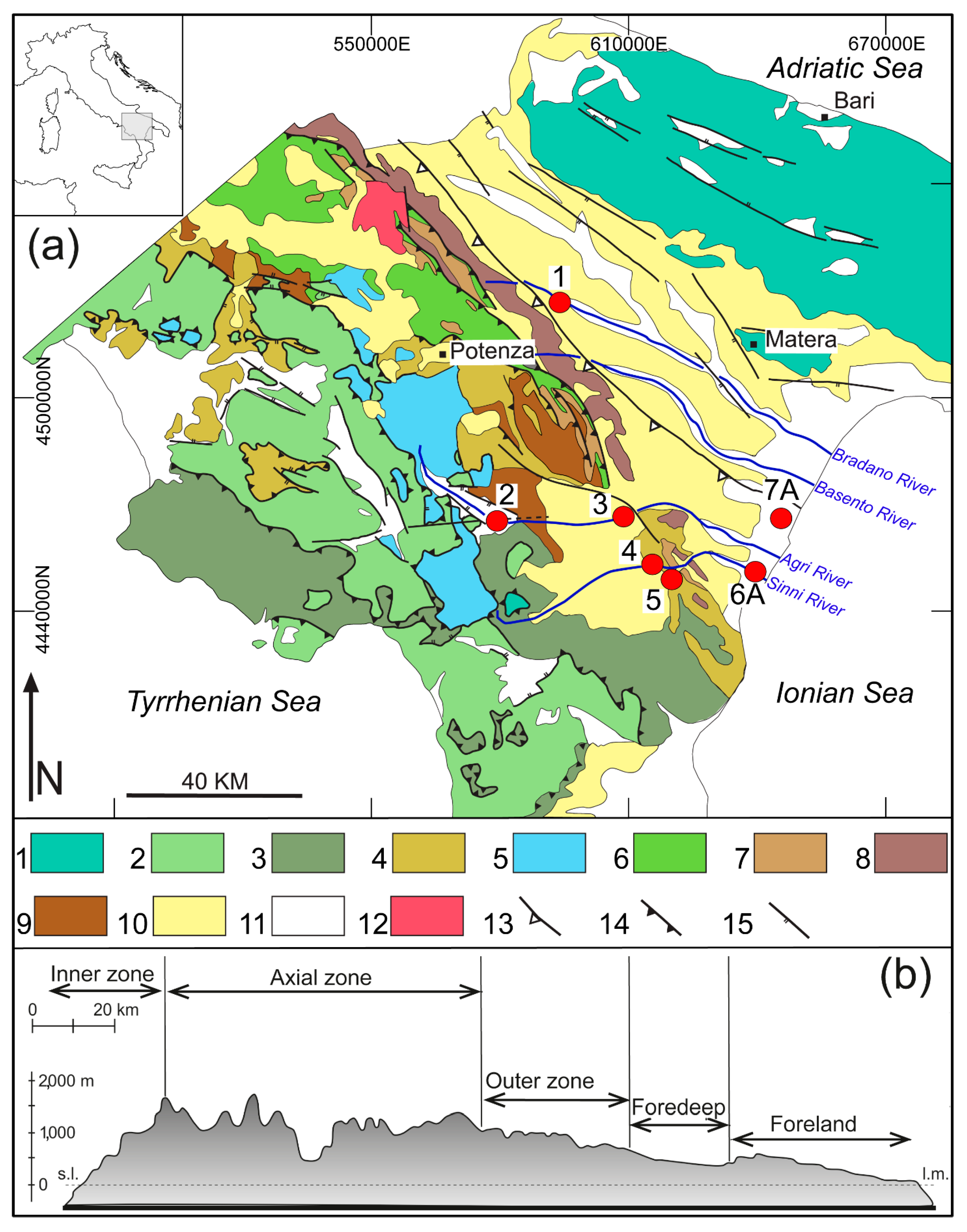
The current physical landscape of Southern Italy is the result of the Miocene-to-Quaternary geological processes shaping the Southern Apennines chain, the Bradano Foredeep, and the Apulian Foreland [31]. The chain is formed by east-verging fold-and-thrust tectonic units [32] overlapped on the Apulian Platform and producing large duplex geometries [31]. The Southern Apennine chain, from geological and morphological points of view, can be roughly divided into three zones: the inner, axial, and outer (Figure 1a,b). The average direction of the chain is about N150°, corresponding to the strike of both the main thrusts and the coaxial normal faults, while extensional tectonics is still active along the axis of the chain-deforming Pleistocene sediments. Such a complex structural setting produced mountain chains over 2000 m high and a NW–SE-oriented regional divide. As a result, the drainage network flows towards the Tyrrhenian Sea (southwest), the Adriatic Sea (northeast), and the Ionian Sea (east). The inner zone corresponds to the Tyrrhenian side of the Southern Apennines and includes Cretaceous-to-Miocene, deep-water carbonate and siliceous, pelagic successions overthrusted on Mesozoic shallow-water platform carbonates units [31]. It corresponds to the Cilento Promontory, with a maximum elevation reached at Cervati Mt. (1900 m a.s.l.). Transverse valleys are cut by rivers flowing toward the Tyrrhenian Sea, locally producing up to 100 m depth of the vertical incision. The axial zone shows high relief with mountain peaks that reach about 2000 m a.s.l. at the Pollino Massif. The geological bedrock in the axial zone is composed by shallow-water carbonate platform units, deep-water siliceous units, siliciclastic arenaceous and clayey units, metamorphic and crystalline units, and clastic successions representing the infill of Pliocene and Pleistocene marine to continental basins [31]. In the axial portion of the chain, fault-related mountain blocks or morphostructures, bounded by high-angle fault scarps, alternate with tectonically induced basins filled by fluvial to lacustrine deposits, which pit the landscape [33,34,35]. Furthermore, the uplift rate of the block-faulted mountain front was not constant in time and space in the Pleistocene continental intermontane basins [34]. The outer zone, representing the imbricate frontal thrust units of the chain, is characterized by hilly reliefs not exceeding 1100 m of altitude. It is formed of arenaceous, marl, silty, and clayey deposits. The easternmost zone corresponds to the Bradano Foredeep, mainly filled with Pliocene-to-Pleistocene conglomerate, sand, and clay successions. The foredeep forms a plain area fairly dipping toward the east and transversally incised by a drainage network [36]. It represents the remnant of a Pleistocene coastal plain uplifted in Quaternary times and vertically incised by streams, as a consequence of the Apennines rise [37,38,39].

The Southern Apennines landscape can be displayed in a SW–NE topographic cross-section, revealing the clear asymmetry of its profile (Figure 1a,b). The highest mountain peaks are markedly located westwards with regard to the regional watershed line. The asymmetry between the highest mountain peaks and the regional divide was responsible for the greater length and the lower mean gradient in the north-eastern flank of the chain than in the south-western one. The different gradient slope of the topographic profile determines a steeper gradient and shorter length of rivers flowing toward the Tyrrhenian Sea than the rivers of the Adriatic and Ionian seas. The WNW–ESE-elongated rivers flowing toward the Ionian sector are the Bradano, Basento, Agri, Cavone, and Sinni (Figure 1a). They cross-cut many morphological thresholds, producing a drainage reorganization of the fluvial network [35,40] as a consequence of the Pleistocene tectonic uplift of the whole Ionian belt [37,39]. High tectonic uplift rates were computed in the axial sector of the chain, which can be attributed to the combined effects of regional uplift and local fault activity [34]. Remnants of low-angle erosion surfaces, corresponding to palaeosurfaces uplifted and displaced by Quaternary faulting activity and intermontane fault-related continental basins, are the main landforms of the axial zone of the Southern Apennines [34,41]. Finally, the main features of the western side are rocky coastal ranges and low coastal plains, which host the main river mouths.

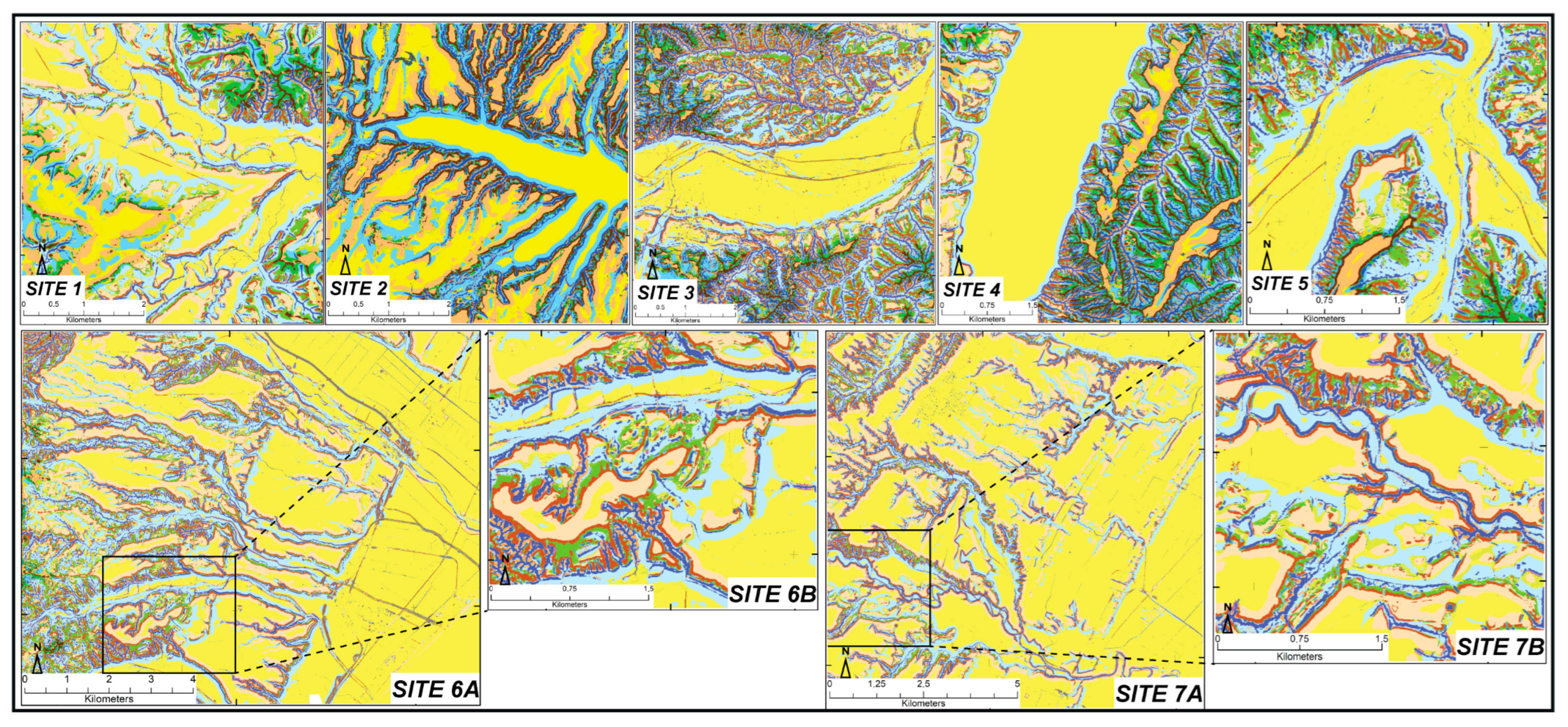
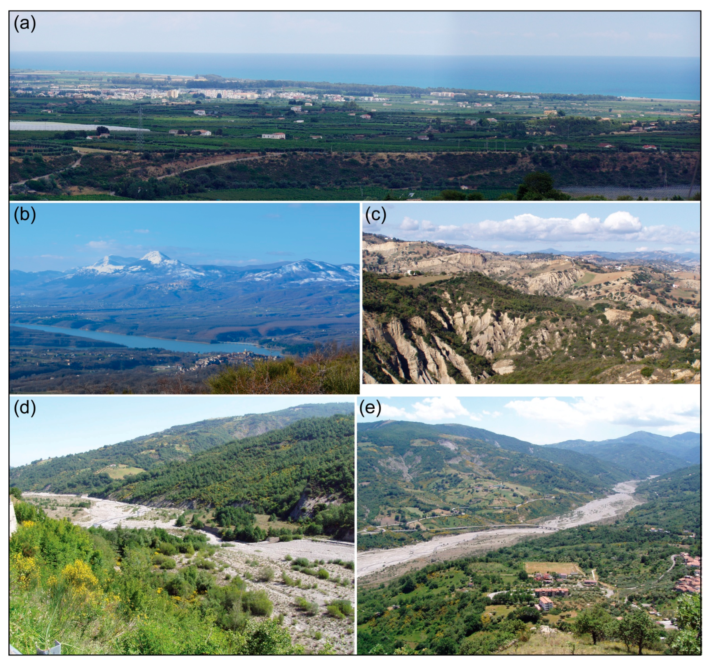
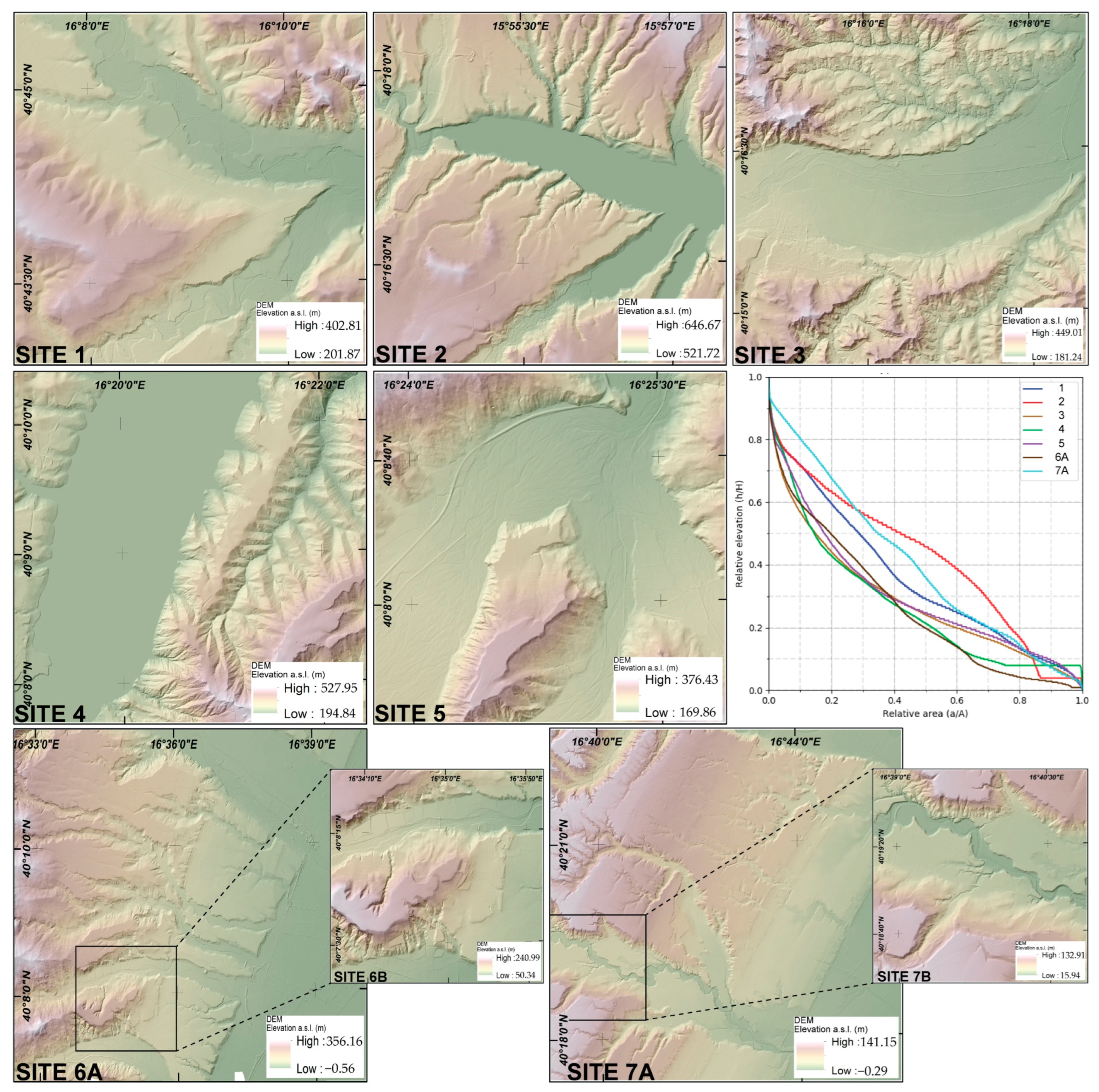
The study area is located in the mid-latitude sector of the Italian peninsula and partly corresponds to the Basilicata Region from a geographical point of view. The physical landscape of the Basilicata Region is composed of different altimetric zones: mountain (46.8%), hill (45.1%), and plain (8%) zones [42]. The elevation ranges from the Ionian Sea to about 2000 m a.s.l. at the Pollino Ridge and the drainage network is eastward-flowing. Flat surface landforms of different origin and age are found within the seven sampled areas and form a staircase sequence of terraces. Flat landforms corresponding to remnants of erosion surfaces are also found in the investigated areas, corresponding to the highest flat surfaces. They are low-angle-tilted landforms ranging from 6° to 12° or more and were not analyzed in the present work. Site 1 represents the northernmost area of investigation and is the upper reach of the Bradano River Valley (Figure 2). It was chosen at the confluence of a tributary in the Bradano River showing two connected floodplains and several orders of fluvial terraces. The area was incised within the Pliocene-to-Pleistocene coarse-grained and thin clastic deposits of the Bradano Foredeep [43]. Site 2 includes the southern sector of the Agri Intermontane Basin, a Pleistocene fault-related trough crossed and incised by the Agri River [36]. The investigation did not consider as a flat surface the Pietra del Pertusillo Water Lake, which is included in the area. Conversely, much of the flat terraced surfaces were formed by the vertical incision of drainage network into the Middle Pleistocene coarse-grained and thin alluvial deposits filling the valley. Site 3 is located in the middle reach of the Agri River Valley and reveals a large floodplain of the thalweg ~2 km wide. Pleistocene clayey and silty deposits make up the two side valleys, and the high rate of denudational processes was responsible for the creation of a badland landscape with “calanchi” and “biancane” landforms [38]. Site 4 is located in the middle reach of the Sinni River Valley, where well-developed relicts of fluvial terraces are found [36]. Site 4 has a large flat surface that corresponds to the Monte Cotugno Water Lake and then was not considered as flat surface. The valley sides are formed of silty-clay deposits with coarse-grained gravel forming the depositional top surface of fluvial terraces. Site 5 displays the lower reach of the Sarmento River Valley, where a tributary flows in the main channel, isolating remnants of high flat surfaces corresponding to old fluvial terraces. The lowest and non-incised flat surface corresponds to the floodplain of the Sarmento River. The site is characterized by the same lithologies of site 4. Both sites 6A and 7A (Figure 2) are situated close to the Ionian Coastal Plain, which is transversally incised by the Sinni (site 6A) and the Cavone (site 7A) Rivers, respectively. The two sites are larger than the previous ones, reaching about 80 km² (site 6A) and 100 km² (site 7A), and contain large remnants of Pleistocene marine terraces, strongly incised by the drainage network [37,39].

3. Materials and Methods

The study area lies in the Southern Italian Apennines chain, where the physical landscape varies from mountain to hills and coastal zones in a low spatial arrangement. It contains flat and low-angle surface landforms, mainly generated by fluvial, marine, and mass movement processes. In selected sampling areas, two combined parameters were used, the best resolution of available DTM, along with two morphometric parameters, the relief and the hypsometry. Ref. [27] compared landform extraction using different resolutions of digital terrain models (DTMs): 5 m, 20 m, and 90 m. They found that the most accurate landform extraction was achieved with the 5 m resolution DTM. In contrast, the 30 m and 90 m resolutions resulted in less accurate outcomes, meaning that some landforms were not detected by the tool, which led to less precise extractions. The 5 m resolution DTM is less time-consuming in the elaboration and provides satisfying results in the mapping visualization [28]. The 5 m resolution DTM of the study area is freely available at https://rsdi.regione.basilicata.it (accessed on 10 May 2024). We used the digital terrain model (DTM) of the Basilicata Region (IT), which is freely available online from the above-mentioned site. The DTM was realized by using an aerial photogrammetric flight from 2013 and was generated by both the ground and model keypoint routines and by a triangulated model z of interpolation. The obtained 5 m resolution DTM was then exported into the ASCII GRID format. The metadata are in UTF8 format, based on the ISO/IEC 10646 standard. The horizontal accuracy of the DTM is 5 m, and the vertical one is 1 m. The information of the DTM metadata are in accordance with the “LineeGuida RNDT” available at the https://rsdi.regione.basilicata.it (accessed on 10 May 2024). The spatial reference of the DTM are related to the Datum ETRS89/UTM-zone33N.

The studied area contains flat and low-angle surface landforms, mainly generated by fluvial, marine, and mass movement processes (see Figure 1a for location areas). Landforms related to mass movement processes were not considered in this study due to the poor outcomes in the semi-automated extraction procedure. Seven small-scale areas were clipped from the DTM, thus producing small patch frames, following the procedure proposed by [22]. The clipping procedure provides small-shaped sites of investigation and allows users to reduce both the computation and the time-consuming nature of the investigation. Small-shaped sites are not recommended because the information provided by the selected patches are not representative of the landscape and topography, furnishing unsatisfactory performances. Conversely, large-shaped patches produce a fast increase in demand of the memory system, and performance will be too slow, thus consuming time. The selection of patch frames includes areas containing both floor and terraced flat surfaces related to fluvial and coastal landscape systems. The frames numbered from 1 to 7 (Figure 1) have a spatial distribution ranging from 25 to 100 km² width. The two frames 6A and 7A, containing very large areas of approximately 80–100 km², were detailed by adding two smaller boxes, 6B and the 7B. The centroid coordinate was used to represent the location of each frame (Figure 2). In selecting the patch frames, we followed the approach utilized in [24,25]. However, we made a distinction by focusing on sampling areas that featured either small or large flat surfaces. Additionally, we aimed to select areas that featured fluvial and/or marine flat surfaces. Furthermore, before the use of the S-G toolbox, the patch frames were preprocessed, filling the “holes” in the raster by using the fill plugin and removing all the small imperfections from the data raster, thus furnishing a new filled surface raster. The next step involved the semi-automated extraction of flat surfaces landforms using GIS application. The clipped and filled DTMs were implemented with the S-G toolbox (version 1.0) [24] running in the ArcGIS application (version 10.7), and the semi-automated extraction and classification of landforms were carried out. 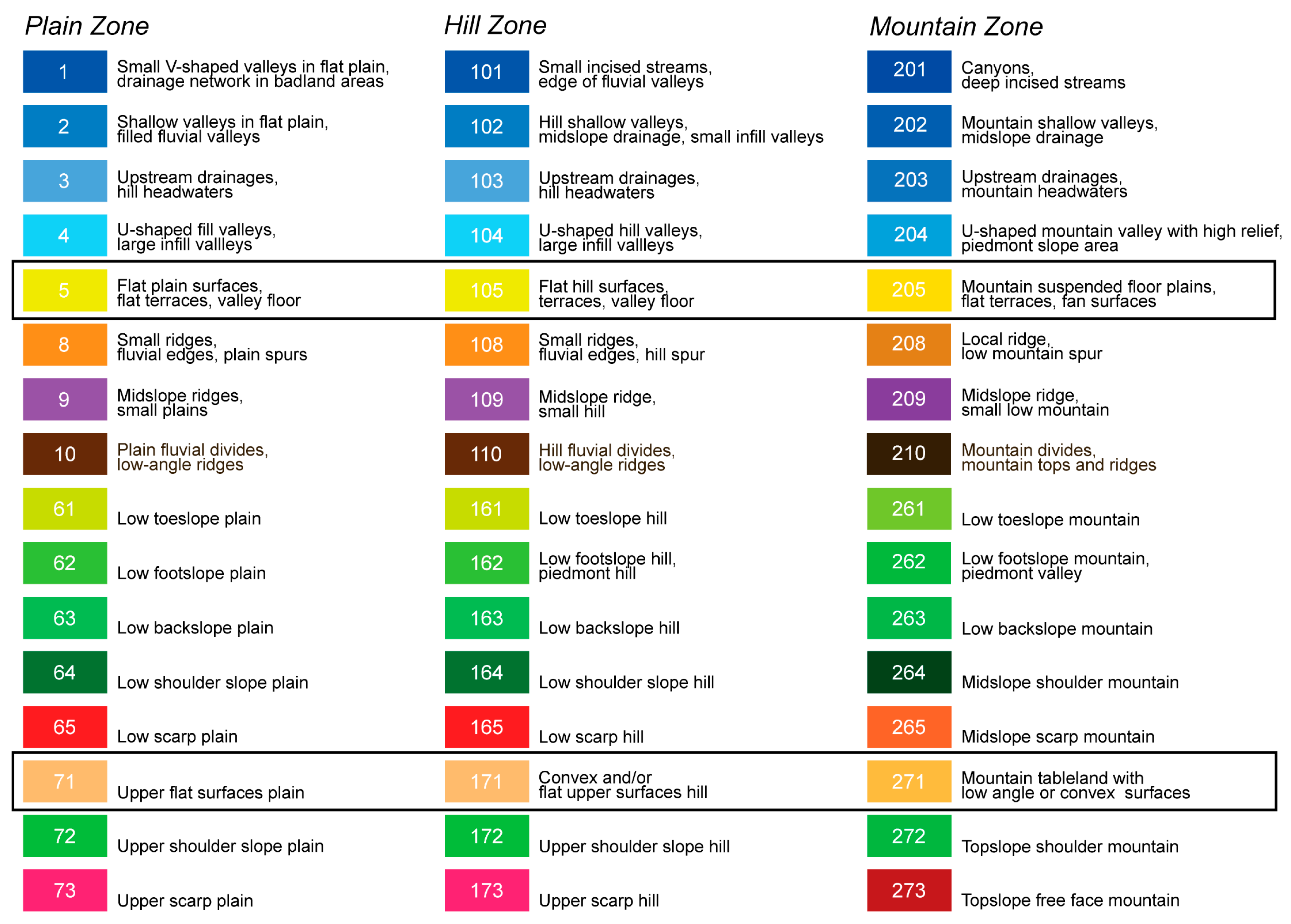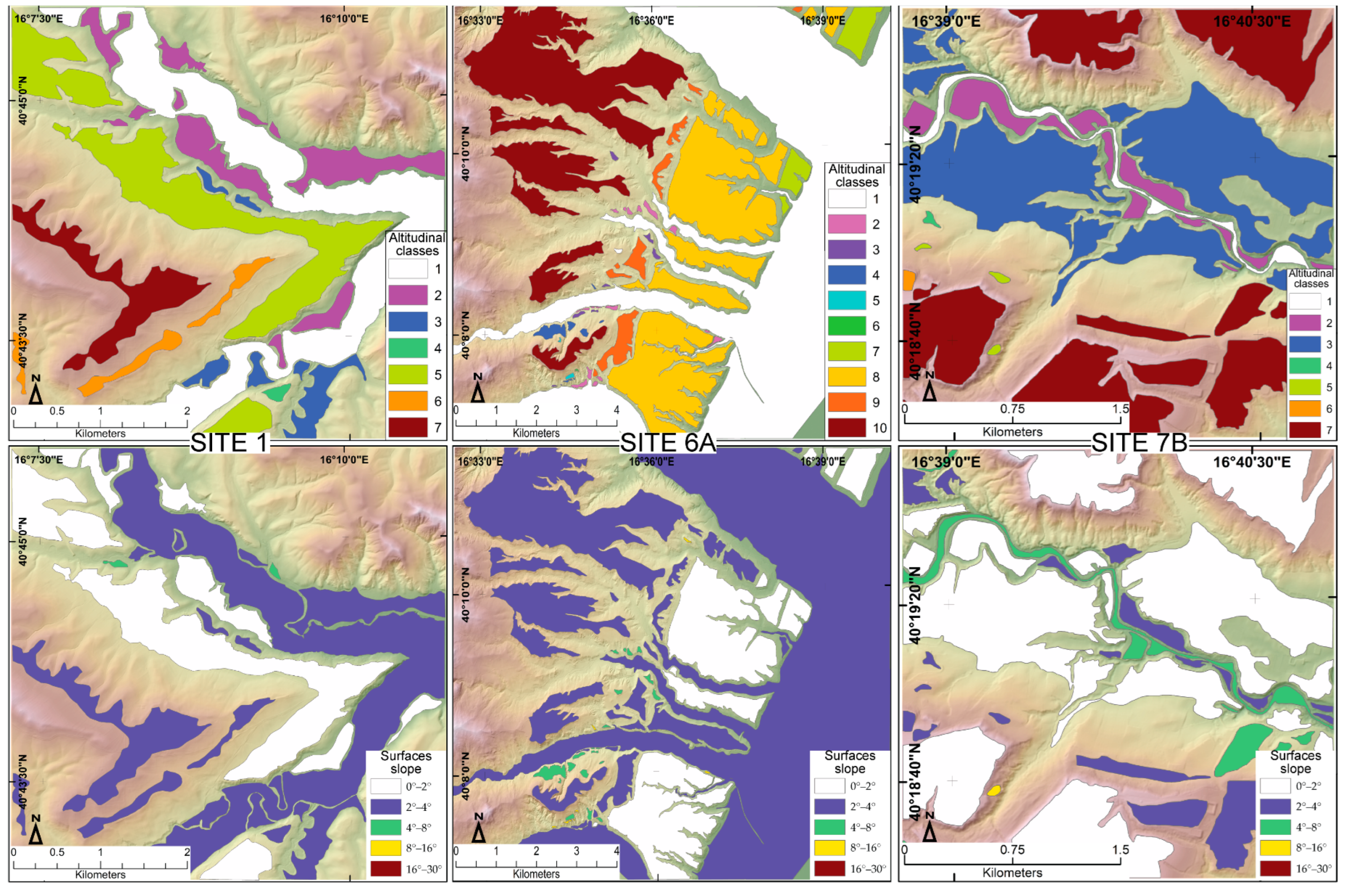The procedure of landforms extraction was based on the topographic position index (TPI) [44] implemented in GIS-based applications [45]. The topographic position index (TPI) is the difference between the elevation value of a cell and the average elevation of the neighborhood around that cell and represents a quantitative relief index. The S-G toolbox (version 1.0) uses six slope classes, starting from the piedmont slope area up to the watershed divide and discriminate landform classes based on the topographic elevation of the physical landscape related to the potential energy of physical processes. This routine process generates a recurrence of landforms combining the altitudinal classes and the six slope angle classes, thus generating the 48 landforms [24] listed in Figure 3.

As a result, the application provides a quick and powerful way to classify landscapes into morphological classes of landforms, and a relevant number of landforms were extracted from the mountain, hill, and plain altimetric zones. Note that each physical landscape in the frame contains only some types of landforms and not all the potential 48 landforms that can be extracted from the tool because of the differences in the topography of landscapes. The flat surface landforms were extracted from the original raster map in a new file using the raster calculator. 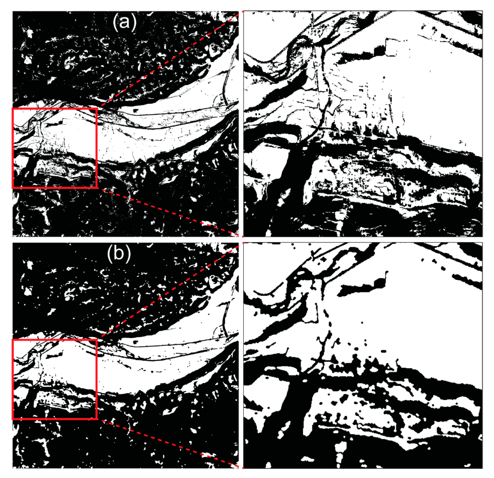The bounding boxes of Figure 3 show the extracted raster of flat surfaces. However, the raster contained many cloud noises linked to small joined pixels, so a cleaning of the raster was necessary. The cleaning procedure was performed using the majority filtering tool found in the ArcGIS Spatial Analyst. By replacing the neighboring cells of similar values in a raster grid with the majority of adjacent cells, the small cells representing the cloud noises were deleted. The filtered raster map’s output is clearer than the original one and free of small clouds. An example of the filtering process applied to site 3 is shown in Figure 4. The difference between the original and uncleaned raster grid (Figure 4a) and the filtered and cleaned raster grid (Figure 4b) is evident, and details are shown in the enlarged right-hand boxes. The best-filtered raster grid was obtained after an iterative filtering process until about 30 extractions. Next, the clean raster grid containing the flat landform types was converted into polygonal features. The polygons were smoothed into simple shapes containing a minimum number of the original raster cell edges. The field parameters of the raster dataset were selected to be used as attributes in the feature classes of the shape files, and the converted polygons not forming flat surface landforms were manually deleted.

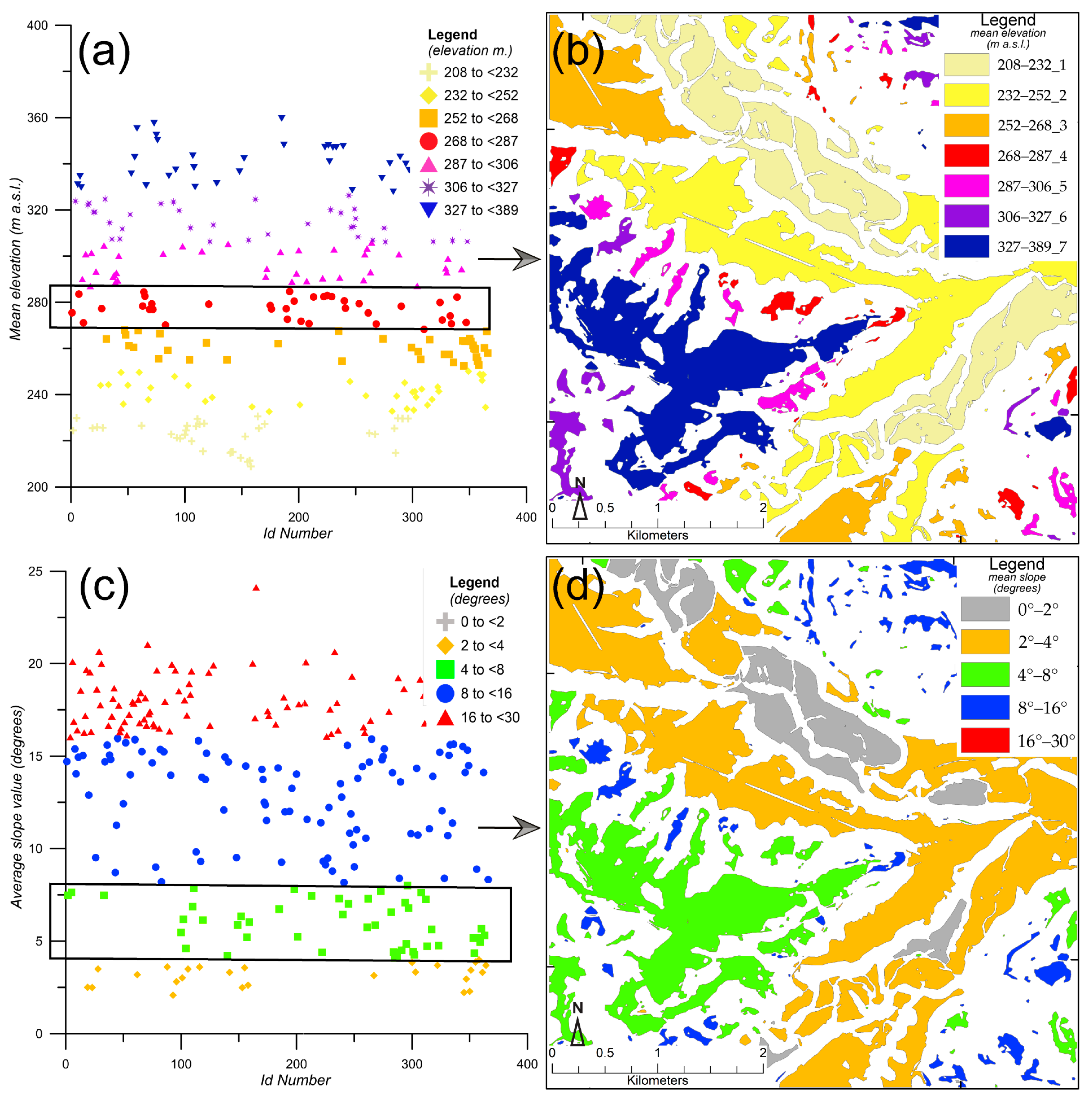
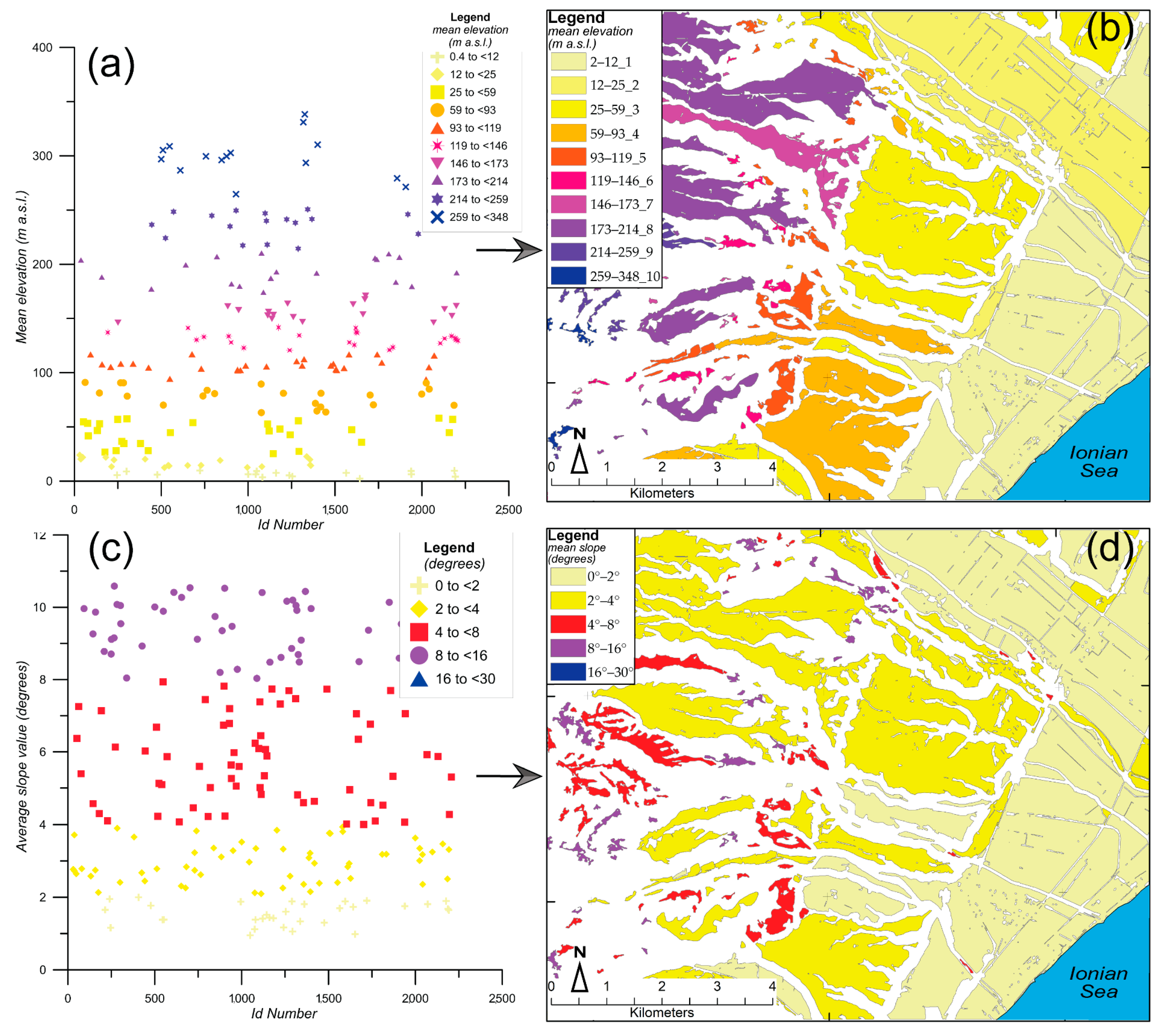
The spatial information (X, Y, Z, and slope degree values) was extracted from each flat surface in the raster DEM using the 3D analyst toolbox of the ArcGIS application. The mean values of Z-elevation and the slope degree were used as morphometric parameters to create homogeneous elevation groups of flat surfaces. Surface values of altitudinal and slope mean values were separately plotted in a scatter class diagram. The altitudinal range values were obtained from an iterative process selecting the best fit distribution of flat surfaces in the scatter plot diagram. Take into account that the selection of cluster surfaces distribution was made manually and then was user-dependent. In terms of slope classifications, [45] defined two slope classes: 0° to 5° and 5° to 90°. In contrast, the new S-G toolbox utilized in [24] categorizes slopes into six classes: 0–5°, 5–12°, 12–30°, 30–60°, 60–75°, and 75–90°. This paper focuses on the first slope class (0–5°) to highlight the presence of flat surfaces. This classification aligns with the standard slope ranges for fluvial and marine environments (0–2°, 2–4°) suggested by several authors [46,47] for non-incised sub-horizontal flat surfaces in fluvial systems as well as [8] for marine systems. Additionally, the next two classes utilized in [24] (5–12° and 12–30°), considering that 30° is the maximum slope for the flat surfaces in the sampled areas, were further divided into three classes (4–8° and 8–16–30°) to emphasize tilted flat surfaces.

The selected classes take into account the local morphology, which varies from hilly to plain. The two slope classes ranging from 0° to 2° and 2° to 4° were assigned to floodplains and coastal plains landforms. The class ranging from 4° to 8° was associated to the slope edge of floodplains and coastal plains, where fan and glacis landforms are present. The slope classes ranging from 8° to 16° and 16° to 30° were related to erosional/depositional talus surfaces and scarps. Surfaces ranging from 16–30° or >30° were interpreted as tilted surfaces triggered by tectonic or gravitative processes acting in the region [37,39] and were not considered. These ranges of slope values were applied in the sampled areas, thus furnishing the slope values distribution of flat and low-angle surfaces. The procedure used in this paper is illustrated in the flow chart of Figure 5.

The geomorphic analysis was realized by field surveys and aerial photos interpretation at a 1:33.000 scale, as furnished by the Italian Geographer Military Institute (I.G.M.I.). In the manual mapping procedure, no software was used. The flat surfaces were analyzed by users, and their interpretation is based on the users’ knowledge. They furnished handmade maps of flat surface landforms that were firstly redrawn with design software and georeferenced and then compared with the automatically extracted flat landforms in the validation process. Furthermore, relief and hypsometry parameters furnished information on the potential energy, lithology, and stage of evolution processes [48]. Local physical landscapes with a mean relief of about 230 m and no abrupt change in the hypsometric curve were considered, suggesting physical landscapes in steady-state conditions [48,49,50,51,52]. The altitudinal distribution of terraced flat surfaces was realized by a visual-based mapping, which takes into account the altimetry and the physical correlations of surfaces. Geomorphic analyses were also used in the attribution of flat surface polygons to fluvial and marine systems. The plan-view perimeter of flat surfaces was detected by analyzing the morphological alignment of landform edges and the changes in slope angle between the terrace tread and the adjacent hillslopes. Comparing the azimuthal line orientation of the frontal scarp terraced surfaces and the azimuthal line orientation of both the coastal line and the main river channels, a morphological attribution to marine or fluvial flat surfaces was firstly carried out. In addition, a field survey random check of the depositional facies of flat surfaces was realized in the field, confirming or not the previous morphological attribution. The automatically extracted flat surfaces elevation and slope maps were then validated through the comparisons of two visual-based maps. The first validation was made by overlapping the extracted flat surface polygons and the handmade flat surface maps produced by field surveys and aerial photos interpretation at a 1:33.000 scale. The second validation took into account the past authorship landform maps, which were overlapped on the automatically extracted landform maps. In addition, the accuracy of the results was verified by assessing three statistical parameters: the correlation coefficient (CC), the root-mean-square error (RMSE), and the coefficient of determination (R²).

4. Results

The semi-automated method of landform extraction enabled automatic recognition of flat surfaces at the investigation sites. Handmade maps of flat surfaces and assessment of morphometric parameters obtained by field survey and aerial photo interpretation were also compared to the semi-automated data. The spatial distribution of flat surfaces made by the semi-automated extraction and by the geomorphic analyses evidenced how fluvial and marine landforms co-exist in transitional areas. Floor flat surfaces correspond to present-day floodplains and coastal plains, whereas terraced surfaces are related to relics of landforms generated during past base levels. Fluvial and marine terraces were generated by a lowering of base levels, producing a staircase distribution of flat surface landforms starting from the coastal zone to the eastern front of the chain. Among the seven sampled areas, those related to sites 1, 6A, and 7B are detailed, showing the best visualization of flat surfaces.

4.1. Semi-Automated Extraction and Classification of Landforms

The GIS-based semi-automated extraction and classification of landforms and their spatial distribution are shown in the sample maps of Figure 6. The yellow color in the maps corresponds to both the floor and non-incised surfaces and the suspended and terraced ones. It is important to point out that the semi-automated extraction did not produce any distinction between fluvial and marine flat surfaces, and their discrimination was performed by integrating the geomorphic features information. Furthermore, not all the 48 landforms listed in Figure 3 were extracted and classified in each frame by the semi-automated procedure. Flat landforms typologies, as defined in the boxes of Figure 3, were selected and extracted in new maps showing just the flat surfaces landforms, such as those represented in sites 1 and 6A (Figure 7). The cleaning of polygons deleted the cloud noises generated by the extraction process (see example in Figure 4), furnishing cleaner maps. It enabled a significant reduction in the number of small flat surfaces, which in many cases could be associated with surfaces from various origins.

The visual inspection of sampled sites showed the presence of two typologies of flat surface polygons: the first are polygons vertically incised by the drainage network and thus forming terraced surfaces, whereas the second are polygons not incised by streams and related to flat surfaces of floor areas; in the latter areas, streams flow on the floor surface. Then, the arrangement of drainage network represents a first factor useful to discriminate between hanged and terraced surfaces from non-incised floor surfaces (Figure 6). Two parameters, the mean Z-elevation and the mean slope values extracted from attribute table of flat surface polygons (Figure 8 and Figure 9 and

Table 2. Scatter classes generated by grouping equal numbers of flat surfaces distributed in a range of average slope values varying from 0° to 30°. FSC: flat surface classes; As: average slope (degrees); PFS: percentage of flat surfaces (%); NFS: number of flat surfaces.

FSC	As	PFS	NFS		FSC	As	PFS	NFS
SITE 1					SITE 6A
1	0–2°	0	0		1	0–2°	1.69	16
2	2–4°	10.12	26		2	2–4°	9.28	88
3	4–8°	19.07	49		3	4–8°	23.95	227
4	8–16°	36.58	94		4	8–16°	35.97	341
5	16–30°	34.24	88		5	16–30°	29.11	276
SITE 2					SITE 6B
1	0–2°	0.53	1		1	0–2°	1.08	1
2	2–4°	8.51	16		2	2–4°	9.68	9
3	4–8°	39.36	74		3	4–8°	40.86	38
4	8–16°	35.64	67		4	8–16°	24.73	23
5	16–30°	15.96	30		5	16–30°	23.66	22
SITE 3					SITE 7A
1	0–2°	0.63	3		1	0–2°	1.51	12
2	2–4°	3.55	17		2	2–4°	12.06	96
3	4–8°	22.34	107		3	4–8°	30.53	243
4	8–16°	34.66	166		4	8–16°	33.17	264
5	16–30°	38.83	186		5	16–30°	22.74	181
SITE 4					SITE 7B
1	0–2°	0	0		1	0–2°	0	0
2	2–4°	1.01	1		2	2–4°	15.18	17
3	4–8°	11.11	11		3	4–8°	21.43	24
4	8–16°	42.42	42		4	8–16°	33.93	38
5	16–30°	45.45	45		5	16–30°	29.46	33
SITE 5
1	0–2°	0	0
2	2–4°	2.75	3
3	4–8°	21.10	23
4	8–16°	36.70	40
5	16–30°	39.45	43

), were plotted in two separated scatter class diagrams. They provide the altitudinal and slope distribution of each flat surface. Based on the best fitting of cluster distribution, the flat surfaces were grouped into classes of elevation and slope (Figure 8a,c and Figure 10).

The flat surfaces in the Bradano River Valley (site 1 in Figure 6) form Y-shape polygons located at the confluence of two rivers floodplain where hanged flat terraced surfaces are distributed at different elevation a.s.l. Seven elevation classes of flat surfaces with a staircase distribution and five slope classes were recognized (Figure 8). The sampled area contains 256 flat surfaces automatically extracted by the tool (Figure 10).

Class 7 represents the upper surface ranging from 327 to 389 m of elevation a.s.l. It corresponds to remnants of the oldest terraces recognized in the area. Slope surfaces ranging from 8° to 16° are the dominant class containing 94 surfaces, whereas the slope class 2–4° includes only 26 flat surfaces. The latter class is the more spatially distributed, and flat surface polygons suggest floor areas. Differently, slope surfaces ranging from 4° to 8° are remnants of the oldest and highest terraces (Figure 8d).

In the Agri Intermontane Basin (site 2 in Figure 6), the sedimentary top surface was vertically incised by streams, forming many irregular polygons that indicate terraced flat surfaces. The tool extracted 187 flat surfaces, forming six elevation classes (Figure 10). The slope class 3 ranging from 4–8° is the main class with 74 surfaces. Note that the yellow polygons of the central sector of the frame show the water level of the Pietra del Pertusillo Lake (site 2 in Figure 6), and it was not considered a flat surface. In the middle reach of the Agri River Valley, the more evident flat surfaces were related to the floor Agri Valley and not incised by the drainage network (site 3 in Figure 6). At site 3, 473 flat surfaces forming ten elevation classes were extracted. Class 5 shows 53 flat surfaces and is the most abundant, ranging from 246 m to 256 m of elevation a.s.l. Two secondary classes, with classes 7 and 9 containing 52 landforms in each, are also present. Large surfaces in the area show the slope angle values included in the ranges of 8–16° (166 surfaces) and 16–30° (186 surfaces). This means that the low-angle slope surfaces are the most abundant and are located at higher elevation. The middle reach of Sinni River Valley has a large floor flat surface, is not incised by streams, and has several terraced surfaces distributed at different elevations a.s.l. (site 4 in Figure 6). Site 4 contains 98 flat surfaces and seven elevation classes, overall. There are no dominant classes because each class has 14 flat surfaces (Figure 10). The same surfaces as the slope classes at site 3 can be observed, suggesting a prevalence of higher and low-angle remnants of terraced surface landforms.

The Sarmento River Valley (site 5 in Figure 6) shows a cuspidate floor flat surface corresponding to a tributary confluence and few terraced surfaces. It contains 108 flat surfaces and forms seven altitudinal classes distributed from 174 m to 361 m of elevation a.s.l. Similarly to the previous site 4, there is no dominance of classes because of the number of surfaces varies from 15 to 16. The most abundant slope classes are 8–16° and 16–30°, suggesting a high distribution of upper and low-angle flat surface landforms. The Sinni Coastal Plain area (site 6A in Figure 6) is larger than the previous ones, corresponding to about 80 km², and its physical landscape contains two different geomorphological systems, the Sinni River mouth and the Ionian Coastal Plain. The largest extracted surface corresponds to the Ionian Coastal Plain (class 1 in Figure 9b), whereas the smaller one is the Sinni River Valley (class 2 in Figure 9b). Both the flat surfaces are floor plain surfaces not incised by streams. In addition, several terraced flat surfaces are distributed in the whole area. The extraction of 206 cleaned flat surfaces enabled us to generate ten altitudinal classes ranging from ~2 m to 338 m of elevation a.s.l. (Figure 9 and Figure 10). Class 5 is the most abundant, with 28 surfaces ranging from 83 m to ~119 m of elevation. Despite a small number of surfaces, the width of the polygons is the highest among the sampled areas. The slope class 8–16°, containing 66 landforms, is the most abundant, followed by the class 2–4° with 58 landforms. The slope class 16–30° is lacking, suggesting the absence of upper and low-angle flat surface landforms in the whole Sinni area. Slope classes 0–2° and 2–4° contain 32 and 58 surfaces, respectively, and can be assigned to floor flat surfaces of the Sinni Floodplain and Coastal Plain (Figure 9d).

An interesting morphological observation is that many slope scarps of terraced surfaces are NE–SW-oriented, aligning with the Ionian coastline direction. Site 6B shows in greater detail characteristics of the site 6A, with about 7.5 km² width and 92 flat surfaces distributed in six classes, ranging from 56 m to 221 m of elevation a.s.l. (Figure 10). No main class was observed because the classes contain 15 or 16 flat surfaces each. The details furnished in this map were useful in the geomorphic analysis of terraces because they were not evidenced in the larger-scale map. As an example, the orientation of lower scarps of terraces is not the same; W–E- and NE–SW-oriented are the main directions of the scarp edges of terraces, suggesting a different morphogenesis of terraced landforms. Site 7A contains the Cavone River mouth and the Ionian Coastal Plain and is the largest frame among the selected ones, reaching about 100 km² (site 7A in Figure 6). The terraced flat surfaces, dissected by streams and forming terraces distributed at different elevations a.s.l., are dominant. The site contains ~383 flat surfaces, forming ten classes distributed from ~1 m to ~135 m of elevation a.s.l. (Figure 10). The altitudinal class 10, ranging from 107 m to 135 m, is the most abundant with 53 flat surfaces. In site 7A, the slope class 8–16° is the most abundant with 114 surfaces, while class 2–4° has 111 surfaces. Flat and low-angle surfaces seem to be the main landforms of the area, with different slope values largely distributed. The detail of site 7B shows seven classes ranging from 21 m to 132 m of elevation a.s.l., with 72 flat surfaces. There is no dominant class because the number of surfaces varies from 6 to 13. Slope values in the whole area range from 2° to 13°, and the slope class 4–8° is the main class with 28 surfaces.

4.2. Geomorphological Analysis of Sampled Sites

The morphological features of sampled sites (see Section 2 for details) combined with the analysis of altitudinal zones, relief, and hypsometry provided information concerning the geomorphic evolution of the landscape. The Bradano River Valley (site 1 in Figure 2) is characterized by a hilly landscape with a relief of ~200 m, suggesting sub-aerial denudational processes with moderate potential energy. In addition, the not-perfect S-shaped form of the hypsometric curve (Figure 2) suggests a low dismantled landscape that has not yet reached the geomorphic equilibrium [45]. The field survey and the aerial photo interpretation enabled identification of 28 flat surfaces with a staircase distribution (Site 1 in Figure 11), a mean elevation ranging from 215 m to 343 m, and a mean slope value ranging from 1° to 5.5°. The lowest flat surface corresponding to the Bradano River Floodplain is placed at about 210 m of elevation a.s.l., whereas the highest is at 357 m. The 28 flat surfaces were grouped into seven altitudinal classes based on the elevation a.s.l. and on physical and geomorphological correlations.

The field survey of some terraces has shown fluvially related conglomerate and sand deposits, and the morphological analysis of the alignment of fluvial scarp edges parallel to the Bradano River Channel revealed the belonging of flat surfaces to the fluvial system. Site 2 is characterized by a relief of ~125 m, suggesting low energy for denudational processes mainly operated by rivers. The S-shaped form of the hypsometric curve (site 2 in Figure 2) indicates it has not yet reached geomorphic equilibrium [48]. Denudational processes at site 3, mainly affecting clayey and silty deposits, were active in a landscape with a relief of ~268 m and were responsible for the concave upward shape of the hypsometric curve (site 3 in Figure 2). The curve indicates a landscape that is prone to a mature stage of evolution [48]. The relief value in site 4 is ~333 m, suggesting a moderate to high energy for denudational processes in a fairly mature landscape, as also indicated by the concave upward form of the hypsometric curve (site 4 in Figure 2). Site 5 shows a relief of ~206 m, indicating a moderate energy for sub-aerial denudational processes active in a fluvial landscape. The not-perfect concave upward form of the hypsometric curve (site 5 in Figure 2) means a not completely mature landscape in which the erosion processes are still locally active. The wideness of both 6A and 7A sites required details of flat landforms that are represented in sub-sites 6B and 7B (Figure 2). Different reliefs were computed in the two main sites: ~356 m in site 6A (Sinni area) and ~141 m in site 7A (Cavone area). Hence, the first has higher denudational processes energy than the second one, as also demonstrated by the more concave upward form of the hypsometric curve of site 6A (Figure 2). Details of field survey and aerial photos analyses are shown in sites 6A and 7B (Figure 11). In the Sinni area (6A), the 85 flat surfaces firstly recognized were grouped into ten altitudinal classes of elevation. The lowest mean elevation is 17 m a.s.l., whereas the highest is 209 m a.s.l. Slope values ranging from 1° to 14° show an eastward dipping of surfaces toward the Ionian Sea in the whole area, as already demonstrated by [39]. Based on geological and geomorphological analyses, ten flat surfaces were identified in the Sinni Coastal Plain and its surroundings (Figure 11). The lowest surfaces in the Sinni area (6A), numbered as 1 in Figure 11, are those related to both the floodplains and the coastal plain areas and may be considered as undifferentiated flat surfaces. Site 7B represents a detail of the Cavone area (7A) and contains 53 flat surfaces (Figure 11). Detailed field surveys and geomorphological consideration on the morphological alignment of scarp edges of terraces permitted to discriminate 13 terraced surfaces attributed to marine environment and 40 to fluvial ones in that area. Moreover, seven altitudinal classes of elevation were recognized. The highest surfaces (numbered as 7), ranging from 57 m to 130 m of elevation a.s.l. and from 1.1° to 6.7° of slope angle, are remnants of marine terraces. The remaining lower surfaces, ranging from 19 m to 110 m of elevation a.s.l. and from 0.6° to 5.2° of slope angle, are fluvially related flat surfaces. In conclusion, the field survey and the geomorphological analyses were useful in both the recognition of floor and non-incised flat surfaces and the vertically incised terraced flat surfaces. In addition, details were furnished on the discrimination between the fluvial than marine origin of the surfaces.

5. Discussion

The use of GIS-based analyses and geomorphic assessments has revealed various landform types in the analyzed Southern Italian landscape. The morphological features of these flat landforms have allowed for their classification into distinct categories of these flat landforms and facilitated their classification into distinct categories. Lower and non-incised flat surfaces were assumed to be floodplains of fluvial systems and coastal plains of marine environments. Flat surfaces showing vertical incisions and terracing were classified as fluvial or marine terraces. This systematic method of classifying landforms enhances our understanding of the geomorphological processes and dynamics that have shaped these areas, providing valuable insights into their environmental history. The morphological attribution of terraced surfaces to fluvial systems was carried out taking into account the following: (i) the scarp edge alignment of terraces parallel to the fluvial talweg, (ii) the flat surfaces that are 20 m higher than the local base levels of thalwegs, and (iii) the physical correlation of terraces along the two sides of the valley. The attribution requires caution and careful control of the altitudinal distribution of terraces using field surveys and aerial photogrammetric analyses. The attribution of terraced surfaces to the marine system are mainly related to the morphological features and the presence of marine depositional facies.

The Sinni Coastal Plain area (site 6A) experienced raising due to the interaction between tectonic uplift and climatic changes during Pleistocene times. Hence, actually, the marine terraces were suspended at different elevations a.s.l. The present-day coastal plain area is bounded inland by small-sized rectilinear scarps representing the inner edges of marine terraces. 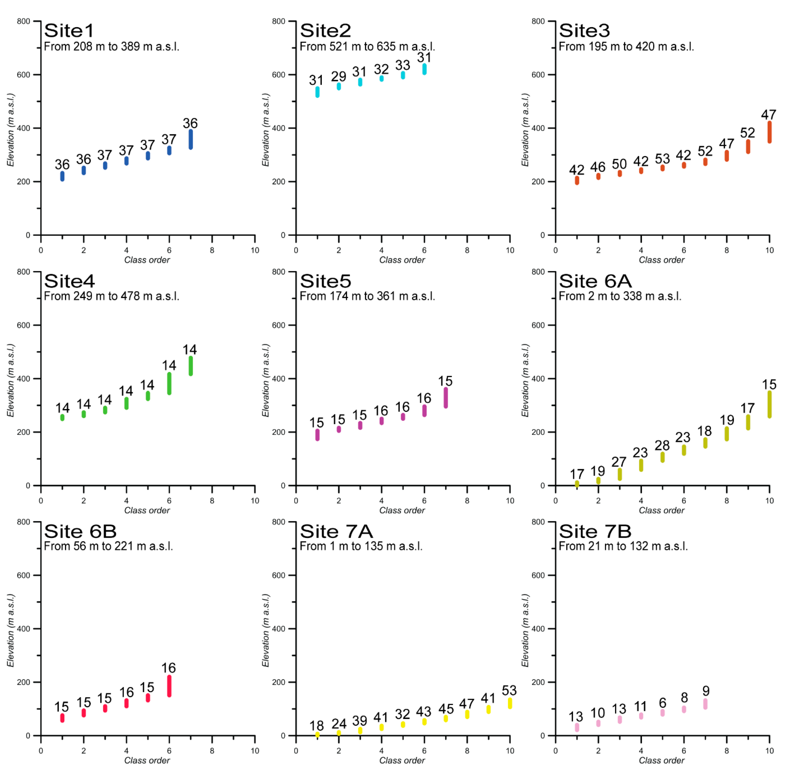The scarps are NE–SW-oriented and nearly parallel to the Ionian coastal line, supporting the evidence of their marine morphogenesis (Figure 7). It is worth noting that the orientation of both the fluvial and marine scarp edges serves as the key morphological marker to distinguish between fluvial and marine terraced surfaces. Scarp edges of fluvial terraces are differently oriented according to the elongation of channel rivers. 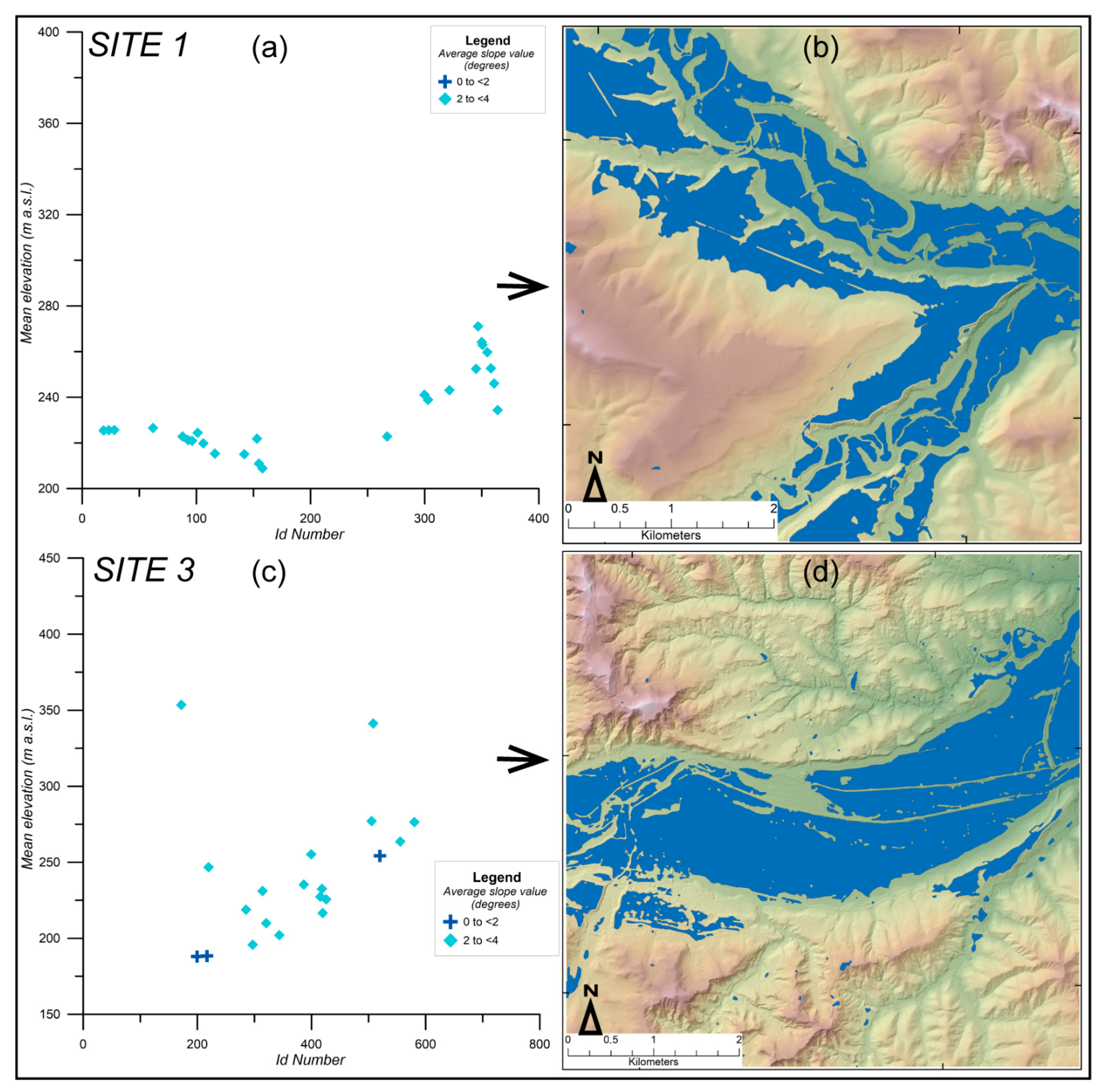The number of elevation classes of terraces measured in the field and by aerial photos varies between 6 and 10 (Figure 6), and the same number of classes was found in the semi-automated extraction of flat surfaces. In the Bradano and Agri Fluvial Valleys (sites 1 and 3, respectively), the semi-automated flat terraced surfaces corresponding to low altitudinal classes of terraces are shown (Figure 12). Terraced surfaces with low slope angles less than 4° are still connected to the present-day floodplains. In addition, the polygons are elongated parallel to the main fluvial valley sides, and the scarps edges are aligned with the main channel line. Right-side terraced surfaces of the Agri Intermontane Basin (site 3) are spatially represented by elevation classes 3, 4, and 5, which are distributed from 256 m to 225 m a.s.l. (Figure 10). In the Sinni River Valley (site 4), the altitudinal classes of terraces 5 and 7 are the most representative, ranging between 346 and 324 m and 478 and 417 m a.s.l. (Figure 10). According to [36], this corresponds to the Piano Codicino and Piano delle Rose Fluvial Terraces, which were deeply incised by the Sinni River in Pleistocene times. The flat surfaces extracted in the river valley floodplain have a slope less than 4°, and their elevation and the elongation of scarp edges parallel to the main channel are the most geomorphic parameters for attributing the related polygons to a fluvial origin. In addition, the creation of elevation classes to differentiate terraces shows a lowering of local base level in the studied area. They represent important parameters to define boundaries within streams that can exist and develop their courses [53]. The geomorphic parameters used in the recognition of fluvial flat surfaces partially correspond to thresholds used by different authors, such as the local gradient and elevation [20] and the local slope and height in DEMs [13].

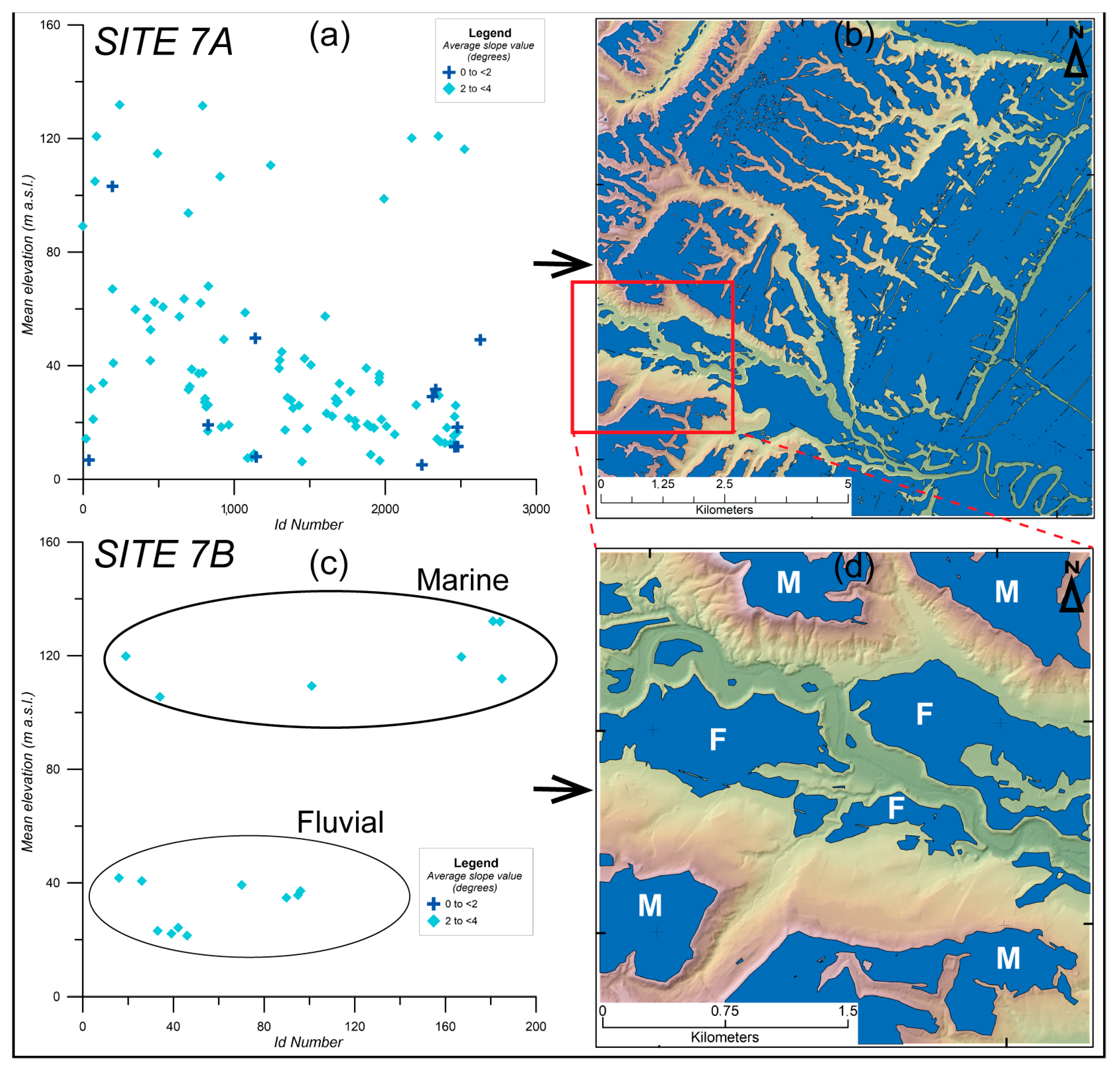
The genetic attribution of flat surfaces in transitional areas, where fluvially and marine-related surfaces crop out, was more complex. Site 6A, including the Ionian Coastal Plain and the Sinni River mouth, evidence surfaces with a slope less than 2° both in the coastal plain and the river floodplain (Figure 9d). Then, the slope of surfaces was unable to distinguish between coastal plain and floodplain. Conversely, the comparison of elevation classes revealed that surfaces of class 1, ranging from 2 to 12 m a.s.l., are elongated parallelly to the coastal line and then correspond to coastal plain surfaces. Surfaces of class 2, ranging from 12 to 25 m a.s.l., show elongation of polygons parallelly to the main river channel and can be most likely attributed to the hanged floodplain of the Sinni riverbed. Other altitudinal classes ranging from 3 to 10 contain remnants of flat or low-angle surfaces distributed from 25 m to 348 m, and from a geomorphological point of view, they are consistent with remnants of the Ionian marine terraces. Similarly, quite all the flat terraced surfaces of site 7A were attributed to remnants of marine terraces, excluding those placed in the fluvial valleys (Figure 13a,b). This is clearly shown in site 7B, along the Cavone River Valley, which contains flat surfaces attributable to fluvial and marine terraces (Figure 13c,d). The scatter class diagram of Figure 13c shows that lower elevation surfaces can be associated with fluvial terraces and the higher ones to marine terraces.

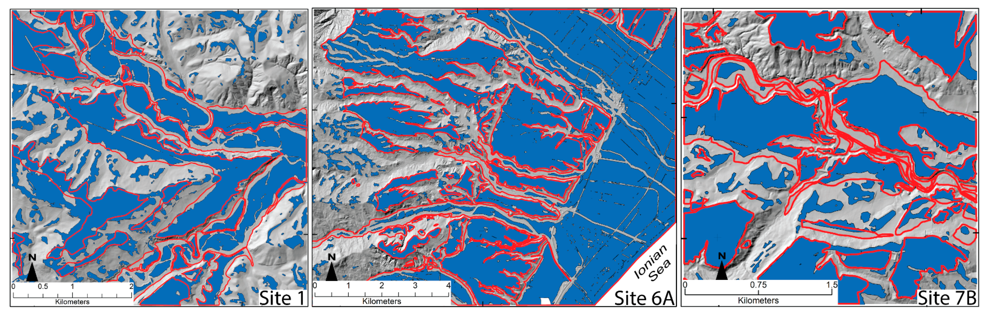
Fieldwork survey maps, such as those shown in Figure 11, were used to validate the spatial distribution of extracted flat surfaces in the sampled sites. The handmade mapping surfaces were used to assess the accuracy of the semi-automated extraction of landforms. The semi-automated flat surfaces of sites 1, 6A, and 7B were overlapped on the handmade flat surfaces of Figure 11 to verify their visual-based correspondence (Figure 14). Results furnished a good fitting, such as in the fluvial system of Bradano River Valley (site 1) and in the marine one of the Ionian Coastal Plain (site 6A). In the detailed map of the Cavone River Valley (site 7B), both the fluvial and marine flat surfaces were overlapped. The visual inspection of the overlapping polygons showed a better fitting of the extracted marine terraces than the fluvial ones. Comparing the flat surface polygons extracted from the GIS and those from the field and aerial photo surveys, it was possible to observe that (i) the semi-automated extraction produced more polygons of flat surfaces than the handmade polygons, and (ii) the polygons area obtained by the semi-automated extraction is smaller than those of the handmade geomorphic analysis. Consequently, the semi-automated extraction of polygons enabled us to obtain better details than the handmade procedure. However, the advantage in obtaining objectively flat surfaces, decreasing its time-consuming nature, shows the disadvantage induced by the error in the semi-automated extraction procedure, which needs to be corrected by users. The flat surfaces of altitudinal class 1 are shown in a panoramic view of the Ionian Coastal Plain, partially corresponding to site 6A (Figure 15a). The arrangement of flat surfaces in the Agri Intermontane Basin (site 2) are found where the floor is divided by the Pietra del Pertusillo Lake (Figure 15b).

The slope angle of the right surfaces is less than 4° and is consistent with the sedimentary top surface of Middle to Late Pleistocene alluvial fans. Figure 15c shows litho-structural horizons forming low-tilting flat surfaces that are related to selective erosion in the Pliocene-to-Pleistocene conglomerates and sands succession of the Sant’Arcangelo Basin (partially corresponding to site 3) [36]. The flat surfaces indicating floodplains and terraces are in the upper reach of Sarmento River in site 5 (Figure 15d,e).

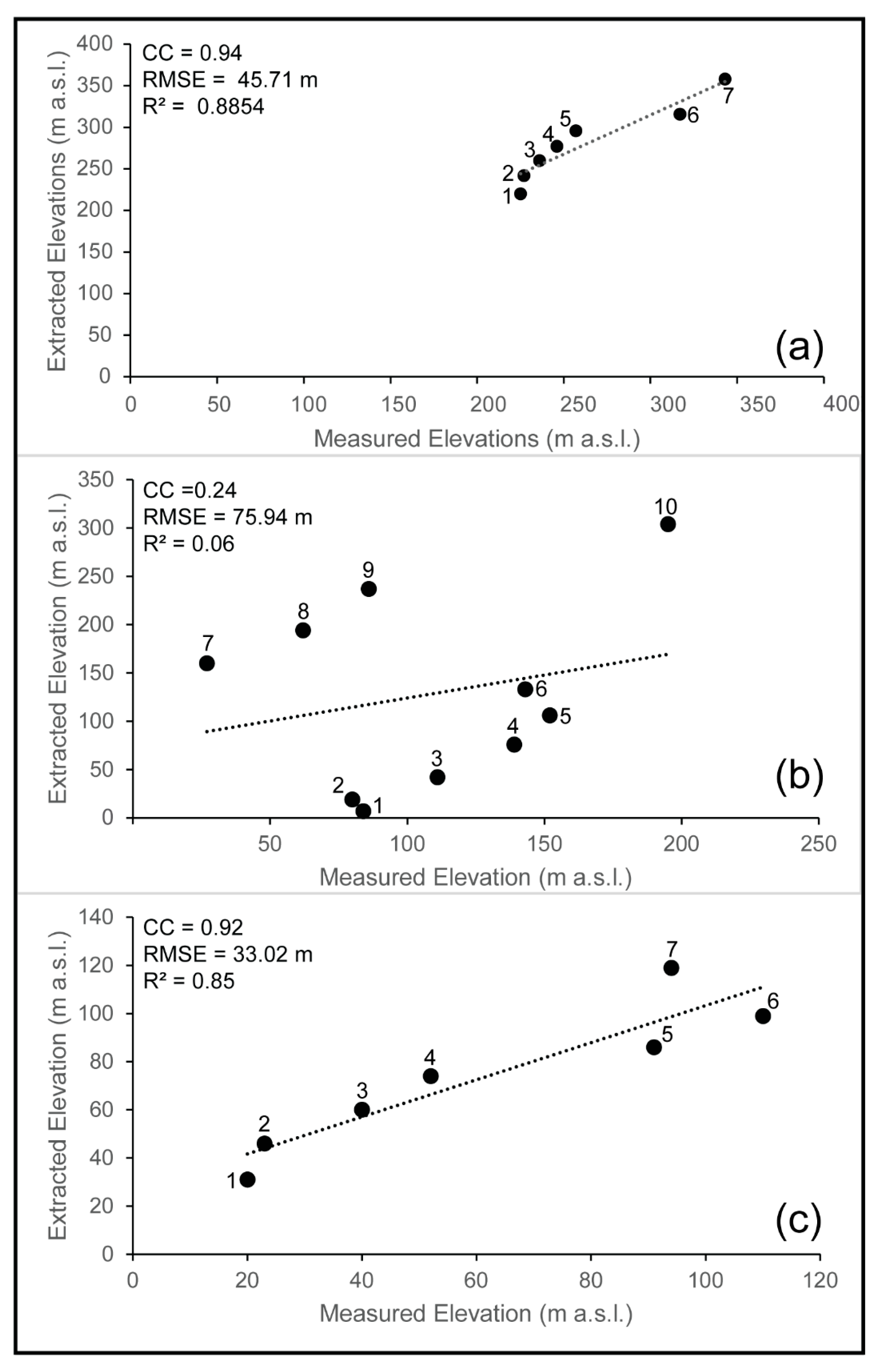
The reliability of semi-automated extraction landforms was tested by plotting the extracted mean elevation classes against the measured classes in a scatter class diagram. Figure 16 displays the relationships between the two mean altitudinal classes related to sites 1, 6A, and 7B. Statistical measurements of correlation coefficient (CC), root-mean-square error (RMSE), and coefficient of determination (R²) were used to assed the accuracy of the method. The indices are indicated as follows:

$$\mathrm{C}\mathrm{C}={\displaystyle \frac{\sum _{\mathrm{i}=\mathrm{i}}^{\mathrm{n}}(\mathrm{E}\mathrm{i}-\mathrm{E})(\mathrm{M}\mathrm{i}-\mathrm{M})}{\sqrt{\sum _{\mathrm{i}=1}^{\mathrm{n}}{(\mathrm{E}\mathrm{i}-\mathrm{E})}^2}\sum _{\mathrm{i}=1}^{\mathrm{n}}{(\mathrm{M}\mathrm{i}-\mathrm{M})}^2}}$$

$$\mathrm{R}\mathrm{M}\mathrm{S}\mathrm{E}=\sqrt{{\displaystyle \frac{\sum _{\mathrm{i}=1}^{\mathrm{n}}{(\mathrm{E}\mathrm{i}-\mathrm{M}\mathrm{i})}^2}{\mathrm{n}}}}$$

$${\mathrm{R}}^2=\mathrm{C}\mathrm{C}\times \mathrm{C}\mathrm{C}$$

where Ei is the mean elevation value computed from the semi-automated extraction, and Mi is the mean elevation value measured by the field survey analyses. E and M are mean values, and n is a record number. CC is the linear correlation between the extracted and measured elevation values and is dimensionless; RMSE is the error between the extracted and the measured values and is expressed in unit of meters; R² measure the goodness of model fit. The accuracy of the semi-automated extraction method was verified in sites 1 and 7B by the CC, RMSE, and R² statistical parameters. A relatively good performance is shown with high CC (CC > 0.92) and R² (R² > 0.85) values. Moreover, small RMSE values (RMSE < 45.71) reinforce the interpretation. The relatively poor performance of site 6A with low CC (CC = 0.24) and R² (R² = 0.06) values is related to the discrepancy between the mean elevations of marine and fluvial terraces. In fact, the higher flat surfaces are marine terraces, whereas the lower ones are fluvial.

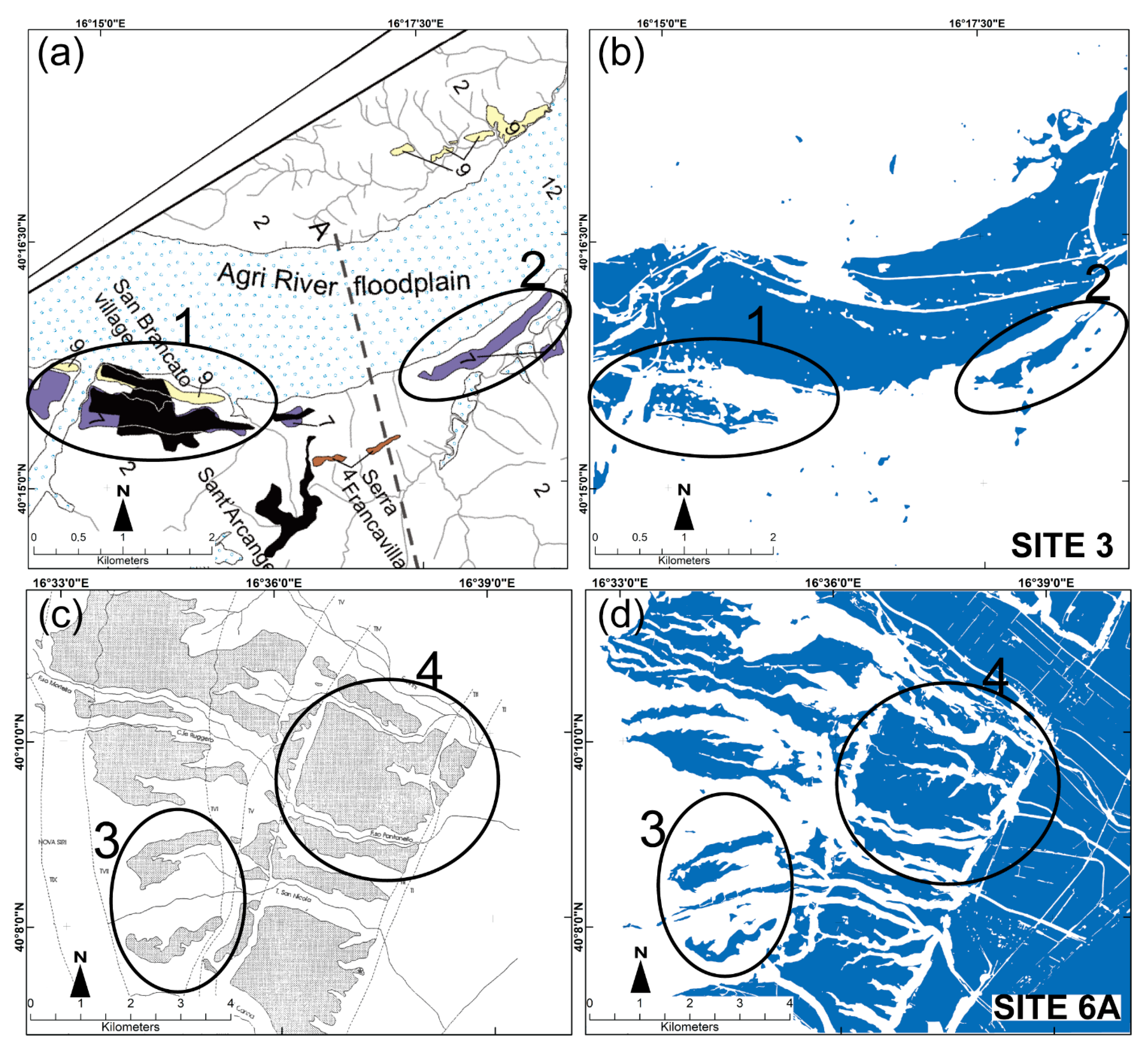
In addition, a visual comparison was carried out between polygons of the semi-automated extracted landforms and the handmade flat surfaces maps. In the middle reach of the Agri Fluvial Valley (site 3), we compared the map of fluvial terraces by [36] with the extracted flat surfaces showing slope angles less than 4° (Figure 17a,b). The floodplain is clearly visible, and two areas numbered as 1 and 2 exhibit the correspondence between the mapped and the extracted fluvial terraces. Similarly, the handmade marine terraces mapped by [54] overlap quite well with the extracted terraces sloping less than 4° from site 6A. Numbers 3 and 4 evidence the quite perfect fitting of marine terraces distributed at different elevations a.s.l. The performance evaluation of three different methods of fluvial terrace extraction proposed by [18] evidenced an overestimation of the terraced surface area. This is a common problem for all automated extractions and was overcome by proposing the mean values of elevation and slope angle of flat surfaces as geomorphic parameters. Ref. [12] extracted geomorphological units in mountainous areas by detecting many types of landforms of various origin. By recognizing a variety of different landforms, a general landform map was achieved instead of a specific detection of a single landform type. Conversely, we selected only flat surfaces, including fluvial and marine landforms, in complex areas such as fluvial valleys and fluvial-coastal plains. In the latter area, the floodplains and fluvial terraces landforms are mixed with the marine landforms. As evidenced in Figure 17, the semi-automated extraction of both the fluvial and marine flat surfaces must be followed by their validation, based on a geomorphological analysis by users. In all cases, the validation process requires a field investigation using analyses of the deposits on which landforms were generated.

6. Conclusions

The study of flat surface landforms in Southern Italy was realized using a GIS-based semi-automated extraction procedure coupled with geomorphic analysis to effectively identify and categorize these features in extensive regions. The research focused on two main categories of flat surfaces: present-day floodplains and coastal plains as well as ancient terraces and low-angle flat landforms. To carry out the investigation, a specialized toolbox within the ArcGIS application was employed [24], which enabled the extraction of landform data that were integrated by the computation of various morphometric parameters and visually represented in scatter class diagrams. These diagrams allowed for a comparative analysis with traditional geomorphological methods, thereby enhancing the validity of the results. The approach provided an easy and fast procedure to automatically obtain flat surfaces containing both the fluvial and marine landforms included in large areas related to coastal and hilly zones of the Southern Italian physical landscape. The findings of this study enhance our understanding of the analyzed physical landscape and highlight the effectiveness of GIS technology in geomorphological research. The validation of the results through comparisons of the extracted flat landform maps with field survey maps and previously published maps yielded several key observations.

-

Quantity and area of polygons: the semi-automated extraction produced a greater number of flat surfaces polygons with smaller areas compared to those drawn using the manual approach;

-

Quality of detail: the semi-automated extraction demonstrated higher detail in the landform representation compared to the handmade procedure;

-

Efficiency: the semi-automated extraction significantly reduced the time required by users to complete the analysis;

-

Error correction: the errors introduced during the semi-automated extraction process needed user intervention for correction;

-

Discrimination of landforms: to really discriminate between fluvial and marine landforms, geomorphological analysis incorporating aerial photos and field survey investigations is necessary.

These observations emphasize the benefits of semi-automated methods in landform mapping while also recognizing the necessity of user oversight and further analyses for specific applications. Recognition and discrimination between fluvial and marine flat surfaces is useful for investigation in low piedmont areas and especially in areas where the transition from continental to marine environments occurs. Identifying these flat landforms can significantly contribute to studies on sea level and fluvial base level oscillations, ecological dynamics, and land-use transitions. This knowledge ultimately aids in improving environmental management and policy decisions. In conclusion, integrating GIS with geomorphic methods for detecting fluvial and marine flat surfaces has proven reliable, even in complex landscapes such as those analyzed in Southern Italy. This approach both deepens our understanding of these environments’ dynamic evolution and aids in making more informed choices in environmental management. It is important to note that territorial management planning conducted without a thorough understanding of these evolutionary dynamics can be ineffective or in some cases detrimental to the environment.

References

1. Thornbury, W.D. Principles of Geomorphology; Wiley: Hoboken, NJ, USA, 1954; p. 594. [Google Scholar]
2. Summerfield, M.A. Global Geomorphology: An Introduction to the Study of Landforms, 1st ed.; Routledge: London, UK, 1991; p. 560. [Google Scholar]
3. Bull, W.B. Geomorphic Response to Climatic Change; Oxford University Press: Oxford, UK, 1991; p. 344. [Google Scholar]
4. Noman, N.S.; Nelson, E.J.; Zundel, A.K. Review of Automated Floodplain Delineation from Digital Terrain Models. J. Water Resour. Plan. Manag. 2001, 127, 394–402. [Google Scholar] [CrossRef]
5. Lewin, J.; Gibbard, P.L. Quaternary river terraces in England: Forms, sediments and processes. Geomorphology 2010, 120, 293–311. [Google Scholar] [CrossRef]
6. Schanz, S.A.; Montgomery, D.R.; Collins, B.D.; Duvall, A.R. Multiple paths to straths: A review and reassessment of terrace genesis. Geomorphology 2018, 312, 12–23. [Google Scholar] [CrossRef]
7. Pazzaglia, F.J. Fluvial terraces. In Treatise on Geomorphology, Fluvial Geomorphology; Shroder, J., Wohl, E., Eds.; Academic Press: San Diego, CA, USA, 2013; Volume 9, pp. 379–412. [Google Scholar]
8. Bird, E. Coastal Geomorphology. An Introduction, 2nd ed.; John Wiley and Sons: Chichester, UK, 2008; pp. 1–411. [Google Scholar]
9. Martha, T.R.; Mohan Vamsee, A.; Tripathi, V.; Kumar, K.V. Detection of coastal landforms in a deltaic area using a multi-scale object-based classification method. Curr. Sci. 2008, 114, 1338–1345. [Google Scholar] [CrossRef]
10. Evans, I.S. Geomorphometry and landform mapping: What is a landform? Geomorphology 2012, 137, 94–106. [Google Scholar] [CrossRef]
11. Minár, J.; Drăguţ, L.; Evans, I.S.; Feciskanin, R.; Gallay, M.; Jenčo, M.; Popov, A. Physical geomorphometry for elementary land surfaces segmentation and digital geomorphological mapping. Earth Sci. Rev. 2024, 248, 104631. [Google Scholar] [CrossRef]
12. van Asselen, S.; Seijmonsbergen, A.C. Expert-driven semi-automated geomorphological mapping for a mountainous area using a laser DTM. Geomorphology 2006, 78, 309–320. [Google Scholar] [CrossRef]
13. Demoulin, A.; Bovy, B.; Rixhon, G.; Cornet, Y. An automated method to extract fluvial terraces from digital elevation models: The Vesdre valley, a case study in eastern Belgium. Geomorphology 2007, 91, 51–64. [Google Scholar] [CrossRef]
14. Bowles, C.J.; Cowgill, E. Discovering marine terraces using airborne LiDAR along the Mendocino-Sonoma coast, northern California. Geosphere 2012, 8, 386–402. [Google Scholar] [CrossRef]
15. Stout, J.C.; Belmont, P. TerEx Toolbox for semi-automated selection of fluvial terrace and floodplain features from LiDAR. Earth Surf. Process. Landf. 2014, 39, 569–580. [Google Scholar]
16. del Val, M.; Iriarte, E.; Arriolabengoa, M.; Aranburu, A. An automated method to extract fluvial terraces from LIDAR based high resolution Digital Elevation Models: The Oiartzun valley, a case study in the Cantabrian Margin. Quat. Int. 2015, 364, 35–43. [Google Scholar] [CrossRef]
17. Eilertsen, R.S.; Corner, G.D.; Hansen, L. Using LiDAR data to characterize and distinguish among different types of raised terraces in a fjord-valley setting. GFF 2015, 137, 353–361. [Google Scholar] [CrossRef]
18. Hopkins, A.J.; Snyder, N.P. Performance evaluation of three DEM-based fluvial terrace mapping methods. Earth Surf. Process. Landf. 2016, 41, 1144–1152. [Google Scholar] [CrossRef]
19. Jara-Muñoz, J.; Melnick, D.; Strecker, M.R. TerraceM: A MATLAB® tool to analyze marine and lacustrine terraces using high-resolution topography. Geosphere 2016, 12, 176–195. [Google Scholar] [CrossRef]
20. Clubb, F.J.; Mudd, S.M.; Milodowski, D.T.; Valters, D.A.; Slater, L.J.; Hurst, M.D.; Limaye, A.B. Geomorphometric delineation of floodplains and terraces from objectively defined topographic thresholds. Earth Surf. Dyn. 2017, 5, 369–385. [Google Scholar] [CrossRef]
21. Zhao, Y.; Wu, P.; Li, J.; Lin, Q.; Lu, Y. A new algorithm for the automatic extraction of valley floor width. Geomorphology 2019, 335, 37–47. [Google Scholar] [CrossRef]
22. Li, S.; Li, K.; Xiong, L.; Tang, G. Generating Terrain Data for Geomorphological Analysis by Integrating Topographical Features and Conditional Generative Adversarial Networks. Remote Sens. 2022, 14, 1166. [Google Scholar] [CrossRef]
23. Brigham, C.A.P.; Crider, J.G. A New Metric for Morphologic Variability Using Landform Shape Classification via Supervised Machine Learning. Geomorphology 2022, 399, 108065. [Google Scholar] [CrossRef]
24. Siervo, V.; Pescatore, E.; Giano, S.I. Geomorphic analysis and semi-automatic landforms extraction in different natural landscapes. Environ. Earth Sci. 2023, 82, 128. [Google Scholar] [CrossRef]
25. Vannametee, E.; Babel, L.V.; Hendriks, M.R.; Schuur, J.; de Jong, S.M.; Bierkens, M.F.P.; Karssenberg, D. Semi-automated mapping of landforms using multiple point geostatistics. Geomorphology 2014, 221, 298–319. [Google Scholar] [CrossRef]
26. Zhang, N.; Fryirs, K. A hierarchical method and workflow for the semi-automated mapping of valley bottom geomorphic units using publicly available remote sensing datasets. Earth Surf. Process. Landf. 2024, 49, 3524–3540. [Google Scholar] [CrossRef]
27. Giano, S.I.; Danese, M.; Gioia, D.; Pescatore, E.; Siervo, V.; Bentivenga, M. Tools for Semi-automated Landform Classification: A Comparison in the Basilicata Region (Southern Italy). In Computational Science and Its Applications. Lecture Notes in Computer Science; Gervasi, O., Murgante, B., Misra, S., Garau, C., Blečić, I., Taniar, D., Apduhan, B.O., Rocha, A.M.A.C., Tarantino, E., Torre, C.M., et al., Eds.; Springer: Cham, Switzerland, 2020; Volume 12250. [Google Scholar] [CrossRef]
28. Cignetti, M.; Godone, D.; Ferrari Trecate, D.; Baldo, M. New Paradigms for Geomorphological Mapping: A Multi-Source Approach for Landscape Characterization. Remote Sens. 2025, 17, 581. [Google Scholar] [CrossRef]
29. Mashimbye, Z.E.; Loggenberg, K. A Scoping Review of Landform Classification Using Geospatial Methods. Geomatics 2023, 3, 93–114. [Google Scholar] [CrossRef]
30. Xiong, L.; Tang, G.; Yang, X.; Li, F. Geomorphology-oriented digital terrain analysis: Progress and perspectives. J. Geogr. Sci. 2021, 31, 456–476. [Google Scholar] [CrossRef]
31. Patacca, E.; Scandone, P. Geology of the Southern Apennines. Boll. Soc. Geol. Ital. 2007, 7, 75–119. [Google Scholar]
32. Pescatore, T.; Renda, P.; Schiattarella, M.; Tramutoli, M. Stratigraphic and structural relationships between Meso-Cenozoic Lagonegro basin and coeval carbonate platforms in southern Apennines, Italy. Tectonophysics 1999, 315, 269–286. [Google Scholar] [CrossRef]
33. Di Leo, P.; Giano, S.I.; Gioia, D.; Mattei, M.; Pescatore, E.; Schiattarella, M. Evoluzione morfotettonica quaternaria del bacino intermontano di Sanza (Appennino meridionale). Alp. Mediterr. Quat. (Il Quat.) 2009, 22, 189–206. [Google Scholar]
34. Giano, S.I.; Gioia, D.; Schiattarella, M. Morphotectonic evolution of connected intermontane basins from the southern Apennines, Italy: The legacy of the pre-existing structurally-controlled landscape. Rend. Fis. Acc. Lincei 2014, 25, 241–252. [Google Scholar] [CrossRef]
35. Giano, S.I.; Schiattarella, M. Drainage integration of small endorheic basins at the Pleistocene-Holocene transition: An example from southern Italy. Geomorphology 2023, 427, 108622. [Google Scholar] [CrossRef]
36. Giano, S.I.; Giannandrea, P. Late Pleistocene differential uplift inferred from the analysis of fluvial terraces (southern Apennines, Italy). Geomorphology 2014, 217, 89–105. [Google Scholar] [CrossRef]
37. Bentivenga, M.; Coltorti, M.; Prosser, G.; Tavarnelli, E. A new interpretation of terraces in the Taranto Gulf: The role of extensional faulting. Geomorphology 2004, 60, 383–402. [Google Scholar]
38. Bentivenga, M.; Giano, S.I.; Piccarreta, M. Recent increase of flood frequency in the Ionian belt of Basilicata region, Southern Italy: Human or climatic changes? Water 2020, 12, 2062. [Google Scholar] [CrossRef]
39. Gioia, D.; Schiattarella, M.; Giano, S.I. Right-Angle Pattern of Minor Fluvial Networks from the Ionian Terraced Belt, Southern Italy: Passive Structural Control or Foreland Bending? Geosciences 2018, 8, 331. [Google Scholar] [CrossRef]
40. Willett, S.D.; McCoy, S.W.; Perron, J.T.; Goren, L.; Chen, C.Y. Dinamic Reorganization of River Basin. Science 2014, 343, 1248765. [Google Scholar] [CrossRef]
41. Giano, S.I.; Schiattarella, M. Age constraints and denudation rate of a multistage fault line scarp: An example from Southern Italy. Geochronometria 2014, 41, 245–255. [Google Scholar] [CrossRef]
42. ISTAT. Circoscrizioni Statistiche. Metodi e Norme; Serie C, n. 1; Abete: Roma, Italy, 1958; pp. 1–239. [Google Scholar]
43. Casnedi, R. La fossa bradanica: Origine, sedimentazione e migrazione. Mem. Soc. Geol. Ital. 1988, 41, 439–448. [Google Scholar]
44. Weiss, A.D. Topographic position and landforms analysis. Poster presentation. In Proceedings of the ESRI User Conference, San Diego, CA, USA, 9–13 July 2001. [Google Scholar]
45. Jenness, J. Topographic Position Index (tpi_jen.avx) Extension for ArcView 3.x, v. 1.2. Jenness Enterprises. 2006. Available online: http://www.jennessent.com/arcview/tpi.htm (accessed on 10 July 2022).
46. Rosgen, D.L. A classification of natural rivers. CATENA 1994, 22, 169–199. [Google Scholar]
47. Fryirs, K.A.; Brierley, G.J. Geomorphic Analysis of River System, An Approach to Reading the Landscape, 1st ed.; Wiley-Blackwell: West Sussex, UK, 2013; pp. 1–345. [Google Scholar]
48. Strahler, A.N. Hypsometric (area–altitude) analysis of erosional topography. Geol. Soc. Am. Bull. 1952, 63, 1117–1142. [Google Scholar]
49. Ohmori, H. Changes in the hypsometric curve through mountain building resulting from concurrent tectonics and denudation. Geomorphology 1993, 8, 263–277. [Google Scholar]
50. Willgoose, G.R.; Hancock, G. Revisiting the hypsometric curve as an indicator of form and process in transport-limited catchment. Earth Surf. Process. Landf. 1988, 23, 611–623. [Google Scholar]
51. Chen, Y.C.; Sung, Q.; Cheng, K.Y. Along-strike variations of morphotectonic features in the Western Foothills of Taiwan: Tectonic implications based on stream-gradient and hypsometric analysis. Geomorphology 2003, 56, 109–137. [Google Scholar] [CrossRef]
52. Walcott, R.C.; Summerfield, M.A. Universality and variability in basin outlet spacing: Implications for the two-dimensional form of drainage basins. Basin Res. 2009, 21, 147–155. [Google Scholar] [CrossRef]
53. Gilbert, J.T.; Macfarlane, W.W.; Wheaton, J.M. The Valley Bottom Extraction Tool (V-BET): A GIS tool for delineating valley bottoms across entire drainage networks. Comput. Geosci. 2016, 97, 1–14. [Google Scholar] [CrossRef]
54. Amato, A.; Belluomini, G.; Cinque, A.; Manolio, M.; Ravera, F. Terrazzi marini e sollevamenti tettonici quaternari lungo il margine ionico dell’Appennino Lucano. Alp. Mediterr. Quat. (Il Quat.) 1997, 10, 329–336. [Google Scholar]
Figure 1. (a) Geological sketch map of Southern Italy. Legend: (1) Apulian platform units (Trias-Paleogene); (2) Apennine platform unit (Trias-Early Miocene); (3) Ligurian unit (Jurassic-Miocene); (4) Sicilian unit (Late Cretaceous-Early Miocene); (5) Lagonegro unit (Trias-Cretaceous); (6) Flysch Rosso Fm (Late Cretaceous-Early Miocene); (7) Flysch Numidico Fm (Early Miocene); (8) Serra Palazzo Fm (Middle-to-Late Miocene); (9) Gorgoglione Fm (Middle-to-Late Miocene); (10) marine to continental units (Late Pliocene-Early Pleistocene); (11) continental units (Middle Pleistocene-Holocene); (12) volcanic unit (Pleistocene); (13) buried thrust front; (14) thrust; (15) high-angle fault. Red dots are the location of selected sites: 1: Bradano River Valley; 2: Agri Intermontane Basin; 3: middle reach of the Agri River Valley; 4: middle reach of the Sinni River Valley; 5: lower reach of the Sarmento River Valley; 6A: Sinni River mouth and Ionian Coastal Plain; 7A: Cavone River mouth and Ionian Coastal Plain. (b) NE–SW-oriented topographic cross-section of Southern Apennines.
Water 17 01022 g001
Figure 2. Shaded relief of the selected frames. In Table 1, both the spatial extent and centroid coordinates of each studied area are reported. Location of sites is indicated in Figure 1. The box on the right side shows the hypsometric curves of sampled sites.
Water 17 01022 g002
Figure 3. Legend of the landforms classification shown in the maps of Figure 6 (modified after [24]). The two bounding boxes are the flat landform typologies, which were selected in the maps.
Water 17 01022 g003
Figure 4. Extraction procedure of the flat surface polygons (a) before and (b) after the filtering process. The sampled area corresponds to the middle reach of the Agri River Valley (site 3). In the right boxes are details of the unfiltered (above) and filtered (below) images (red squares).
Water 17 01022 g004
Figure 5. Flow diagram showing the procedure of landforms detection adopted in this study. Blue color is the input data, light green is the first output data, yellow is the tools, dark green is the secondary output data.
Water 17 01022 g005
Figure 6. Landform maps extracted by the semi-automated process. See Figure 1 for sites location and coordinates and Figure 3 for colors legend.
Water 17 01022 g006
Figure 7. Examples of extracted flat surface maps in sites 1 (a) and 6A (b). Yellow color is the cleaned surfaces after the filtering process, and black color is the cloud noises before the filtering process, which were deleted. The box on the right contains details of the sites.
Water 17 01022 g007
Figure 8. Flat surfaces automatically extracted from site 1 in the Bradano River Valley. Elevation classes of the flat surfaces are shown in the legends of the scatter plot diagrams (a) and the landform map (b). Slope angle classes are shown in the legend of the scatter plot diagrams (c) and the landform map (d). Black boxes in (a) and (c) are examples of the clustering distribution of flat surfaces related to class 4 and class 4–8°, respectively.
Water 17 01022 g008
Figure 9. Flat surfaces automatically extracted from site 6A in the Sinni Coastal Plain. Elevation classes of flat surfaces are shown in the legends of the scatter plot diagrams (a) and the landform map (b). Slope angle classes are shown in the legends of the scatter plot diagrams (c) and the landform map (d).
Water 17 01022 g009
Figure 10. Altitudinal distribution a.s.l. of the flat surfaces in the sampled areas. Above the columns is the number of surfaces pertaining to each group. Classes order is numbered from 1 to 10 and starts from the left of the diagrams.
Water 17 01022 g010
Figure 11. Examples of the handmade flat surface maps realized by field survey and aerial photos interpretation in the three relevant sites 1, 6A, and 7B. Elevation (above) and slope (below) polygons of flat surfaces are shown.
Water 17 01022 g011
Figure 12. Scatter plot diagrams showing the altimetric distribution of the flat surfaces ranging from 0° to 4° (a,c) and the related map distribution (b,d). Boxes (a,b) are related to the Bradano Fluvial Valley (site 1) and (c,d) to the Agri Fluvial Valley (site 3).
Water 17 01022 g012
Figure 13. Scatter plot diagrams showing the altimetric distribution of the flat surfaces ranging from 0° to 4° (a,c) and the related map distribution (b,d). Boxes (a,b) are related to the Cavone Coastal Plain (site 7A), and (c,d) show details.
Water 17 01022 g013
Figure 14. Overlapping of the semi-automated (blue fields) and the field survey (red lines) flat surface polygons in the Bradano River Valley (site 1), Sinni Coastal Plain (site 6A), and detail of the Cavone Coastal Plain (site 7b).
Water 17 01022 g014
Figure 15. Panoramic views of flat surfaces within the studied areas. (a) Ionian Coastal Plain in the Sinni area (site 6A); (b) fluvial terraces in the Agri Intermontane Basin (site 2); (c) low-angle and lithostructural flat surfaces of the Aliano site in the middle reach of the Agri River Valley (site 3); (d) floodplain and fluvial terraces in the Sarmento Stream (site 5); (e) floodplain of the Sarmento Stream (site 5).
Water 17 01022 g015
Figure 16. Diagrams of the extracted vs. measured mean elevation classes. (a) Bradano River Valley (site 1); (b) Sinni Coastal Plain (site 6A); (c) detail of the Cavone Coastal Plain (site 7B). Numbers in the plots refer to the elevation classes of flat surfaces.
Water 17 01022 g016
Figure 17. Comparison between map of terraces already published (a,c) and flat surfaces automatically extracted in the present paper (b,d). Sites are located in the Agri Fluvial Valley (a,b) and in the Sinni Coastal Plain (c,d). Dark circles correspond to the compared areas.
Water 17 01022 g017