Assessment of Future Rainfall Quantile Changes in South Korea Based on a CMIP6 Multi-Model Ensemble

Abstract

Climate change presents considerable challenges to hydrological stability by modifying precipitation patterns and exacerbating the frequency and intensity of extreme rainfall events. This research evaluates the prospective alterations in rainfall quantiles in South Korea by employing a multi-model ensemble (MME) derived from 23 Global Climate Models (GCMs) associated with the Coupled Model Intercomparison Project Phase 6 (CMIP6) under four Shared Socioeconomic Pathways (SSP1-2.6, SSP2-4.5, SSP3-7.0, SSP5-8.5). Historical rainfall data from simulations (1985–2014) and future projections (2015–2044, 2043–2072, and 2071–2100) were analyzed across a total of 615 sites. Statistical Quantile Mapping (SQM) bias correction significantly enhanced the accuracy of projections (RMSE reduction of 63.0–85.3%, Pbias reduction of 93.6%, and R² increase of 0.73). An uncertainty analysis revealed model uncertainty to be the dominant factor (approximately 71.87–70.49%) in the near- to mid-term periods, and scenario uncertainty increased notably (up to 5.94%) by the end of the century. The results indicate substantial temporal and spatial changes, notably including increased precipitation in central inland and eastern coastal regions, with peak monthly increases exceeding 40 mm under high-emission scenarios. Under the SSP2-4.5 and SSP5-8.5 scenarios, the 100-year rainfall quantile is projected to increase by over 40% across significant portions of the country, emphasizing growing challenges for water resource management and infrastructure planning. These findings provide critical insights for water resource management, disaster mitigation, and climate adaptation strategies in South Korea.

1. Introduction

Climate change has significantly altered global precipitation patterns, particularly affecting regions that are especially vulnerable to extreme rainfall events [1,2]. South Korea, situated in the mid-latitudes of East Asia, faces increasing risks due to its unique geographical and climatological characteristics. The country’s distinct seasonal precipitation distribution, primarily influenced by the East Asian monsoon system, results in 60–70% of its annual rainfall occurring during the summer months (from June to August). This phenomenon makes South Korea particularly susceptible to the impacts of extreme rainfall events and their associated consequences [3,4].

Recent events highlight the vulnerability of the region. The unprecedented rainfall during the summer of 2020 resulted in significant flooding, causing extensive damage to infrastructure and agricultural systems, as well as loss of life [5,6]. These incidents underscore the urgent need to understand and predict the effects of climate change on future precipitation extremes in South Korea. This knowledge is crucial for effective infrastructure planning, disaster preparedness, and the formulation of climate adaptation strategies [7].

Rainfall quantiles, which are statistical thresholds representing the amounts of precipitation that are exceeded with designated probabilities, are essential parameters in the fields of hydrological design and risk assessment. These quantiles are essential in the design of critical infrastructure, such as dams, bridges, and drainage systems, and are generally established according to designated return periods, such as events with a 100-year or 200-year recurrence interval [8,9]. However, alterations in precipitation patterns attributed to climate change pose significant challenges to conventional methods of quantile estimation, which have historically operated under the assumption of stationary rainfall patterns over time. Research conducted at 37 weather stations throughout South Korea indicates that 22 of these locations now display unstable precipitation patterns, while only 4 exhibit stability [10]. This observed instability diminishes the reliability of historical data for future predictions, thereby necessitating the development of novel approaches to quantile estimation.

Previous research utilizing earlier climate models (CMIP3 and CMIP5) has identified trends in extreme precipitation associated with global warming [11,12]. Studies conducted by Sperber et al. [13] and Wang et al. [14] projected an increase in heavy rainfall events during monsoon seasons; however, significant uncertainties persisted across various models and scenarios.

The latest Coupled Model Intercomparison Project Phase 6 (CMIP6) provides enhanced climate simulations characterized by higher spatial resolutions and improved representations of physical processes [15]. However, comprehensive studies employing CMIP6 models to evaluate future changes in rainfall quantiles in South Korea are still limited. Preliminary analyses indicate that CMIP6 models may exhibit different climate sensitivities and precipitation patterns compared to their predecessors, underscoring the necessity for a renewed assessment that utilizes these updated datasets [16,17,18,19].

This study addresses a critical research gap by evaluating future changes in South Korea’s rainfall quantiles using bias-corrected precipitation data from the CMIP6 multi-model ensemble (MME). The approach integrates advanced bias correction techniques to align model outputs with observed precipitation patterns, comprehensive regional frequency analysis that accounts for spatial correlations and regional climate characteristics, and multi-model ensemble analysis to capture uncertainties across models and emissions scenarios. The findings aim to provide reliable projections of extreme precipitation changes, supporting climate adaptation strategies, infrastructure design standards, and risk management policies. These results will be instrumental in enhancing South Korea’s resilience to climate-induced hydrological risks in the coming decades.

2. Methodology

2.1. Study Area

South Korea, located in East Asia, occupies the southern portion of the Korean Peninsula between 33 and 39° N latitude and 124 and 130° E longitude. Surrounded by water on three sides, its geographic position significantly shapes its maritime climate patterns (see Figure 1). The country covers an area of 100,210 square kilometers, with over 70% of its terrain characterized by mountainous regions that play a pivotal role in shaping local weather and ecological systems. The annual average temperatures on the Korean Peninsula fluctuate between approximately 11 °C and 14 °C, influenced by regional and topographical differences. Concurrently, the annual precipitation levels generally vary from around 1000 to 1800 mm [20]. South Korea experiences a temperate monsoon climate with four distinct seasons. Summers (June–August) are particularly notable, contributing to 50–60% of the annual precipitation due to the influence of the East Asian monsoon system. However, climate change has introduced increasing irregularities in precipitation, highlighting the growing importance of water resource management and agricultural planning.

While situated at mid-latitudes, South Korea’s climate is moderated by its maritime location and surrounding ocean currents. Winters are often dominated by cold spells associated with the Siberian high-pressure system, whereas summers are characterized by hot and humid conditions driven by the North Pacific high-pressure system. Based on the Köppen–Geiger climate classification system, most areas in South Korea are categorized as having a humid continental climate (Dwa), which is defined by hot, humid summers and cold, dry winters [21].

Geologically, the Korean Peninsula is predominantly composed of Precambrian metamorphic and igneous rocks, with Paleozoic and Mesozoic sedimentary formations present in certain areas. These geological characteristics contribute to the mountainous landscape and play a significant role in shaping regional hydrology and soil properties, which, in turn, impact land utilization, agricultural practices, and the distribution of habitats [22]. The interplay of mountainous terrain, maritime influences, and monsoon systems makes South Korea a critical region for studying climate change in East Asia. Its unique environmental conditions provide valuable insights into the broader impacts of global climate variability, offering guidance for agricultural practices, urban planning, and water resource management as climate patterns continue to evolve.

2.2. Datasets

The rainfall data used in this study were collected and managed by the Korea Meteorological Administration (KMA), the Korea Water Resources Corporation (K-water), and the Ministry of Environment (MOE). All datasets were obtained from the Water Resources Management Information System (WAMIS) [23].

The Earth System Grid Federation (ESGF) provides a comprehensive platform for accessing global climate model (GCM) data produced by research institutions worldwide, serving as a vital resource for climate and Earth science research. This study utilizes daily precipitation simulation data based on climate change scenarios, with detailed information summarized in

Table 1. List of CMIP6 GCMs used in this study.

No.	GCMs	Institution (Nation)	Resolution (km)	Key References
1	ACCESS-CM2	CSIRO-ARCCSS (Australia)	250	Bi et al. [24]
2	ACCESS-ESM1-5	CSIRO-ARCCSS (Australia)	250	Ziehn et al. [25]
3	AWI-CM-1-1-MR	AWI (Germany)	100	Semmler et al. [26]
4	BCC-CSM2-MR	BCC (China)	250	Wu et al. [27]
5	CanESM5	CCCma (Canada)	500	Swart et al. [28]
6	CMCC-CM2-SR5	CMCC (Italy)	100	Cherchi et al. [29]
7	CMCC-ESM2	CMCC (Italy)	100	Lovato et al. [30]
8	EC-Earth3-Veg	EC-Earth-Consortium (Sweden)	100	Wyser et al. [31]
9	EC-Earth3-Veg-LR	EC-Earth-Consortium (Sweden)	250	Döscher et al. [32]
10	FGOALS-g3	CAS (China)	250	Li et al. [33]
11	GFDL-ESM4	NOAA-GFDL (USA)	100	Held et al. [34]
12	IITM-ESM	CCCR-IITM (India)	250	Swapna et al. [35]
13	INM-CM4-8	INM (Russia)	100	Volodin et al. [36]
14	INM-CM5-0	INM (Russia)	100	Volodin et al. [37]
15	IPSL-CM6A-LR	IPSL (France)	250	Lurton et al. [38]
16	KACE-1-0-G	NIMS-KMA (South Korea)	250	Lee et al. [39]
17	MIROC6	MIROC (Japan)	250	Tatebe et al. [40]
18	MPI-ESM1-2-HR	MPI-M (Germany)	100	Gutjahr et al. [41]
19	MPI-ESM1-2-LR	MPI-M (Germany)	250	Mauritsen et al. [42]
20	MRI-ESM2-0	MRI (Japan)	100	Yukimoto et al. [43]
21	NorESM2-LM	NCC (Norway)	250	Seland et al. [44]
22	NorESM2-MM	NCC (Norway)	100	Seland et al. [44]
23	TaiESM1	AS-RCEC (Taiwan)	100	Lee et al. [45]

.

This study employed four SSP and Representative Concentration Pathway (RCP) scenarios: SSP1-2.6 (SSP126), SSP2-4.5 (SSP245), SSP3-7.0 (SSP370), and SSP5-8.5 (SSP585). The SSP126 scenario represents a low-emission pathway characterized by rapid equitable development with minimal environmental impact, aiming to limit global warming to below 2 °C by 2100. SSP245 depicts a medium-emission pathway, reflecting moderate and equitable development with some environmental improvements, resulting in the stabilization of warming to approximately 3 °C by 2100. SSP370 represents a high-emission pathway marked by uneven development, increased conflict, environmental degradation, and a projected temperature rise of around 5 °C by 2100. Finally, SSP585 denotes a very high-emission scenario driven by rapid inequitable economic growth, high energy consumption, and significant emissions, leading to a projected warming of about 6 °C by 2100.

In this study, the simulation period for climate change spanned from 1985 to 2100. For analysis by outlook periods, the timeline was divided into four 30-year intervals: the historical period (S0: 1985–2014), the near-term future period (S1: 2015–2044), the mid-term future period (S2: 2043–2072), and the far-term future period (S3: 2071–2100).

2.3. Bias Correction

GCMs are fundamental to climate change projections. However, their relatively low spatial resolution, typically 100–500 km, leads to significant uncertainties when applying these models to specific basins. To resolve this discrepancy between GCM resolution and the finer scale of hydrological processes, spatial disaggregation and bias correction techniques are utilized. Due to variations in resolution among different GCMs, the initial preprocessing phase requires the standardization of spatial resolution using spatial interpolation techniques such as inverse distance weighting (IDW) [46]. This spatial disaggregation process transforms GCM outputs from coarse resolutions to finer scales using methods like statistical downscaling or dynamical downscaling with regional climate models. This approach effectively produces a uniform grid resolution suitable for basin-scale applications while bridging the gap between large-scale climate patterns and local-scale hydrological responses.

For bias correction, we focus on the widely adopted Quantile Mapping (QM) approach, which adjusts model outputs using the cumulative probability distributions of observed and simulated data. Basic Quantile Mapping assumes specific theoretical probability distributions (e.g., normal or gamma distributions) for both the observed and model data to perform bias correction. The fundamental principle can be expressed as follows:

$$x_{corrected}=F_{obs}^{-1}\left(F_{mod}\left(x_{mod}\right)\right)$$

(1)

where $F_{obs}$ and $F_{mod}$ represent the cumulative distribution functions (CDFs) of observations and model data, respectively, and $F_{obs}^{-1}$ is the inverse CDF of observations.

Non-parametric Quantile Mapping differs from the basic approach by avoiding assumptions about specific probability distributions, instead relying on empirical distributions [47]. This method better captures the actual distributional characteristics of the observed and modeled data, making it particularly useful for correcting extreme values and handling complex distribution patterns. Additionally, it enables the development of separate mapping functions for different months or seasons, allowing for a more accurate representation of seasonal variations. Non-parametric Quantile Mapping is widely used in climate model downscaling and is particularly effective for correcting biases in climate variables with complex distributions [48]. The bias correction employed in this research was conducted utilizing the ‘qmap’ package, which is accessible in the R (version 4.4.3) programming environment [49].

2.4. Regional Frequency Analysis

Frequency analysis of hydrologic data involves statistically estimating the probability and magnitude of past extreme events using probability distributions. This study employs the Regional Frequency Analysis (RFA) methodology, which integrates Index Flood Methodology (IFM) based on the Generalized Extreme Value (GEV) distribution and the L-moments approach, as outlined in the Standard Guidelines for Estimating Flood Quantiles in Korea [50]. The resulting probability-based rainfall estimates serve as critical inputs for evaluating the effectiveness of rainfall-runoff models.

The GEV distribution is a commonly employed probabilistic model for conducting frequency analysis. The PDF and CDF associated with the GEV distribution are presented in the following equations:

$$\mathrm{PDF} :f\left(x\right)={\displaystyle \frac{1}{\alpha }}{\left[1-{\displaystyle \frac{\beta \left(x-x_0\right)}{\alpha }}\right]}^{\left(1/\beta \right)-1}\exp \left[-{\left(1-{\displaystyle \frac{\beta \left(x-x_0\right)}{\alpha }}\right)}^{1/\beta }\right]$$

(2)

$$\mathrm{C}\mathrm{DF} :F\left(x\right)=\exp \left[-{\left(1-{\displaystyle \frac{\beta \left(x-x_0\right)}{\alpha }}\right)}^{1/\beta }\right]$$

(3)

where $x_0$, $\alpha$, and $\beta$ are the location, scale, and shape parameters, respectively.

2.5. Performance Evaluation

In order to assess the effectiveness and accuracy of the General Circulation Models (GCMs) employed in this study, we implemented a range of statistical indices. The root mean square error serves as the primary indicator of overall model error; however, we also compared using additional metrics, namely percent bias and the coefficient of determination, to enable a more thorough evaluation of model performance. The following sections will outline each metric and provide its respective mathematical formulation.

2.5.1. Root Mean Square Error (RMSE)

The RMSE quantifies the average magnitude of discrepancies between the observed and simulated values, placing a relatively greater emphasis on larger errors. A lower RMSE signifies a closer alignment with the observed data. The RMSE is mathematically defined as follows:

$$\mathrm{RMSE}=\sqrt{{\displaystyle \frac{1}{n}}\sum _{i=1}^n{\left({Obs}_i-{Sim}_i\right)}^2}$$

(4)

where ${Obs}_i$ represents the observed value, ${Sim}_i$ denotes the model-simulated value at time step $i$, and $n$ is the total number of observations.

2.5.2. Percent Bias (Pbias)

Percent bias (Pbias) serves to quantify the average inclination of the simulations to either overestimate or underestimate their corresponding observations. A negative Pbias indicates a tendency for the model to overestimate, whereas a positive Pbias suggests an underestimation of the observations. The Pbias is expressed as follows:

$$\mathrm{Pbias}=\left[{\displaystyle \frac{{\sum }_{i=1}^n\left({Obs}_i-{Sim}_i\right)}{{\sum }_{i=1}^n{Obs}_i}}\right]\times 100\%$$

(5)

A Pbias value of zero indicates a perfect correspondence between the simulated and observed values, with values approaching zero reflecting improved model performance.

2.5.3. Coefficient of Determination (R²)

The coefficient of determination (R²) is a dimensionless metric that evaluates the extent to which the simulated values correspond to the variability observed in the data. R² ranges from 0 to 1, with values nearer to 1 indicating a superior fit. It is calculated using the following formula:

$${\mathrm{R}}^2={\displaystyle \frac{{\left[{\sum }_{i=1}^n\left({Obs}_i-\overline{Obs}\right)\left({Sim}_i-\overline{Sim}\right)\right]}^2}{\left[{\sum }_{i=1}^n{\left({Obs}_i-\overline{Obs}\right)}^2\right]\left[{\sum }_{i=1}^n{\left({Sim}_i-\overline{Sim}\right)}^2\right]}}$$

(6)

where $\overline{Obs}$ and $\overline{Sim}$ represent the mean value of the observed and simulated data, respectively.

3. Results

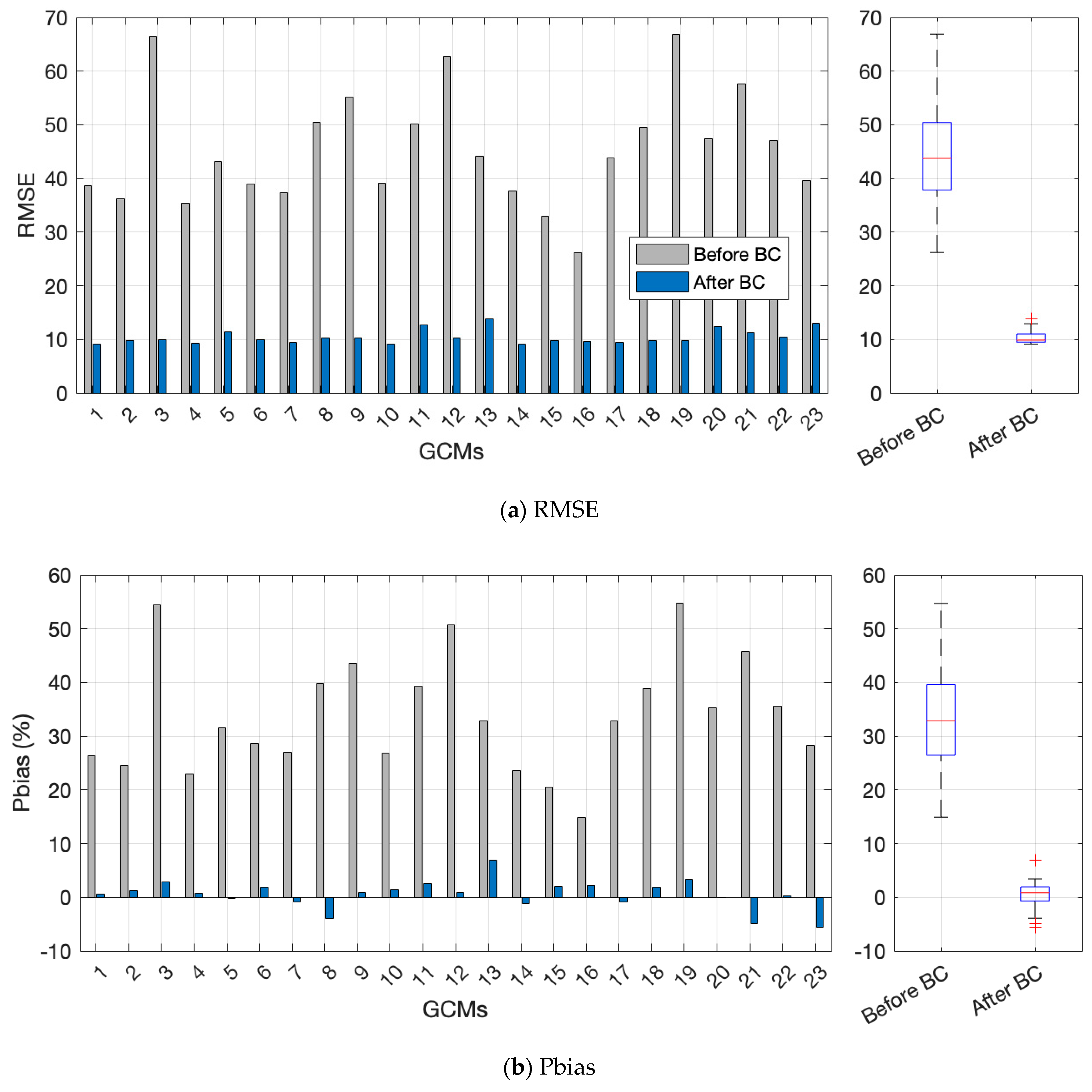
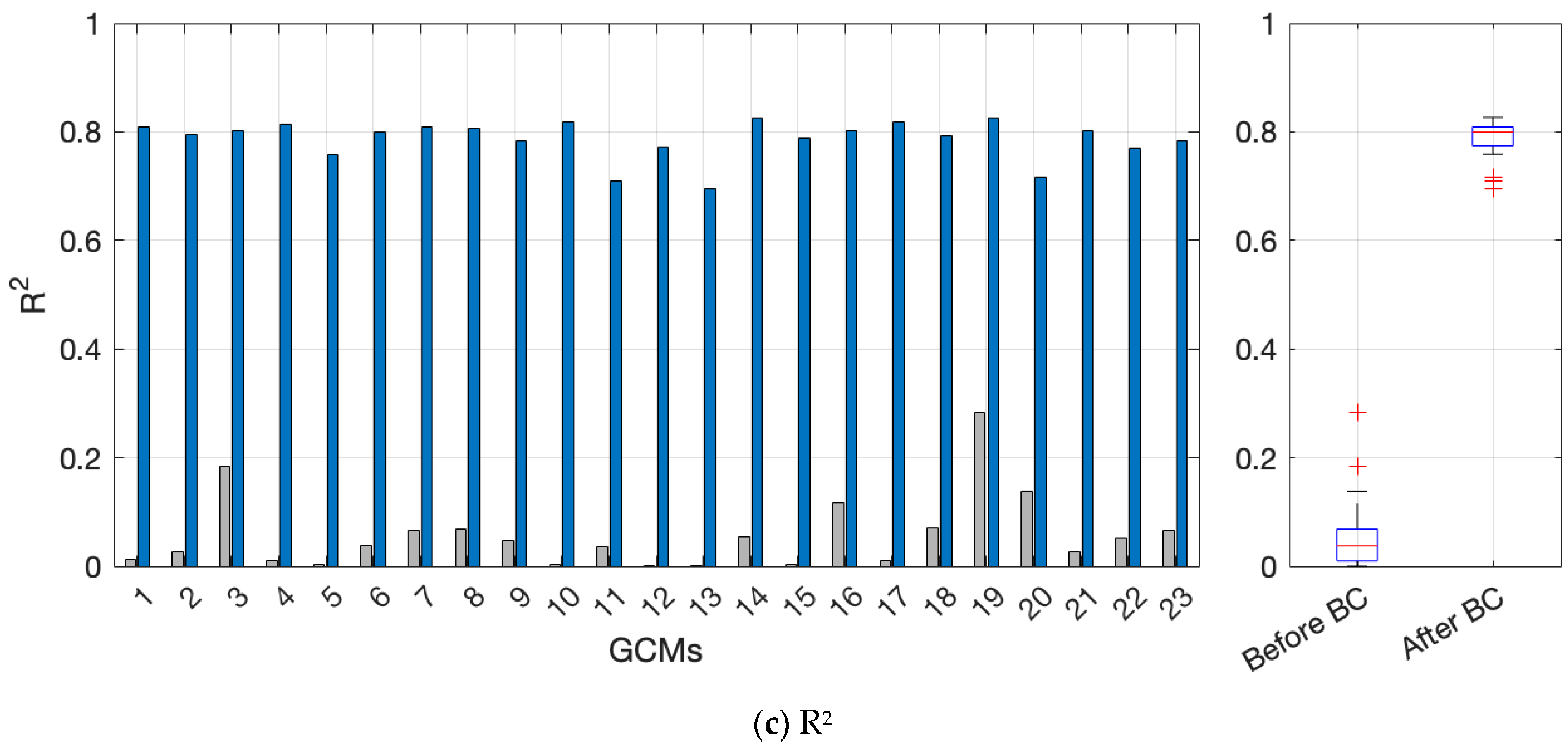
3.1. Historical Verification

Before projecting future scenarios, it is essential to evaluate how effectively bias correction methods improve the accuracy of climate models in simulating historical observed data. We evaluated the climate models’ raw and bias-corrected data to verify their consistency with the observed data. In this study, Statistical Quantile Mapping (SQM) was applied to the outputs of 23 GCMs. SQM adjusts the statistical distribution of model outputs to align more closely with the observed data, thereby correcting systematic biases.

Figure 2 illustrates the RMSE, Pbias, and R² of each GCM before (gray bars) and after (blue bars) SQM bias correction. Calculations were based on data from 615 sites across the study area. RMSE quantifies the difference between model predictions and observed data, with lower values indicating better alignment with observations.

Before bias correction, significant variability in GCM performance is evident, as shown in Figure 2a. The application of SQM significantly reduces RMSE values across all models. For example, the model (GCM 19) with an initial RMSE of 66.9 improves dramatically to approximately 9.8 after bias correction. Even the best-performing model (GCM 16) is further refined, with its RMSE decreasing from 26.2 to about 9.7. The right side of Figure 2a presents a boxplot summarizing the RMSE of all 23 GCMs before and after SQM. The median RMSE of the GCMs decreases from approximately 43.8 before correction to 9.9 after correction, demonstrating that SQM effectively mitigates the biases inherent in the GCMs.

In addition, Figure 2b presents the Pbias, which indicates how much each model overestimates or underestimates the observed values. Before bias correction, most GCMs showed substantial positive biases, leading to large deviations from the observations. However, after bias correction, Pbias values generally moved closer to 0%, indicating that overestimations were significantly reduced.

Figure 2c displays the R², which measures how well the model output explains the variability in the observations. Prior to bias correction, most GCMs exhibited very low R² values, whereas after correction, R² increased markedly for the majority of the models. This improvement points to a strengthened correlation between the models’ outputs and observed data, highlighting the enhanced explanatory power of the bias-corrected models. Taken together with the RMSE results, these findings demonstrate that the bias correction method not only reduces errors, but also effectively improves model bias (Pbias) and goodness-of-fit (R²).

To quantify the improvements achieved using the SQM bias correction method, the percentage reduction in RMSE was calculated for each GCM. This metric provides a standardized and comparable measure of the effectiveness of bias correction in aligning climate model outputs with observations. Figure 3 illustrates the percentage enhancements in RMSE and Pbias, as well as the absolute increase in R², for all 23 GCMs. The RMSE values for these 23 GCMs exhibited improvements between 63.0% and 85.3%, indicating that the SQM approach effectively reduces systematic biases and yields results that are more closely aligned with the observed data. Even the model with the lowest improvement showed a substantial 63.0% improvement, with an average improvement of 76.0%. These results highlight the significant benefits of SQM bias correction in enhancing the reliability of GCM outputs for climate change projections.

The consistency of these improvements across all GCMs is particularly noteworthy, with all models showing improvements over 60%. This robustness underscores the wide applicability of SQM in addressing systematic biases, regardless of the individual model’s characteristics or baseline performance. Furthermore, the high percentage reductions in RMSE indicate that the corrected climate scenarios are far more accurate and reliable than their uncorrected counterparts.

In addition to the RMSE, enhancements in Pbias were also assessed to evaluate the degree to which the outputs of the models correspond to the observed values in terms of bias. Among the 23 General Circulation Models (GCMs) analyzed, the percentage improvement in Pbias varied from 79.2% to 99.9%, with an average improvement of approximately 93.6%. This finding suggests that the SQM bias correction method significantly mitigates both positive and negative biases, thereby facilitating a closer alignment of climate models with the observed data. Furthermore, the absolute increase in the R² was measured to quantify the extent to which the corrected outputs align with the variance in observed measurements. The analysis indicated a minimum increase of approximately 0.54 and a maximum increase of about 0.81, yielding an average increase of around 0.73. Given that R² values range from 0 to 1, this absolute difference underscores the considerable enhancement in the model’s capacity to represent observed variability following the application of SQM bias correction.

Collectively, these supplementary metrics bolster the assertion that SQM not only diminishes overall error, as indicated by the RMSE, but also systematically addresses bias (Pbias) and enhances the overall fit to observed variability (R²). By utilizing multiple evaluation metrics, this study illustrates that SQM provides substantial performance improvements across various dimensions of model accuracy and reliability. These substantial improvements in accuracy have critical implications for water resource impact assessments that rely on GCM outputs. By enhancing the reliability of climate change scenarios, the SQM bias correction method enables water resource managers and policymakers to make more informed decisions. In conclusion, the percentage reductions in RMSE presented in Figure 3 provide compelling evidence of the effectiveness and importance of applying SQM bias correction to GCM outputs, ensuring more accurate and robust climate projections.

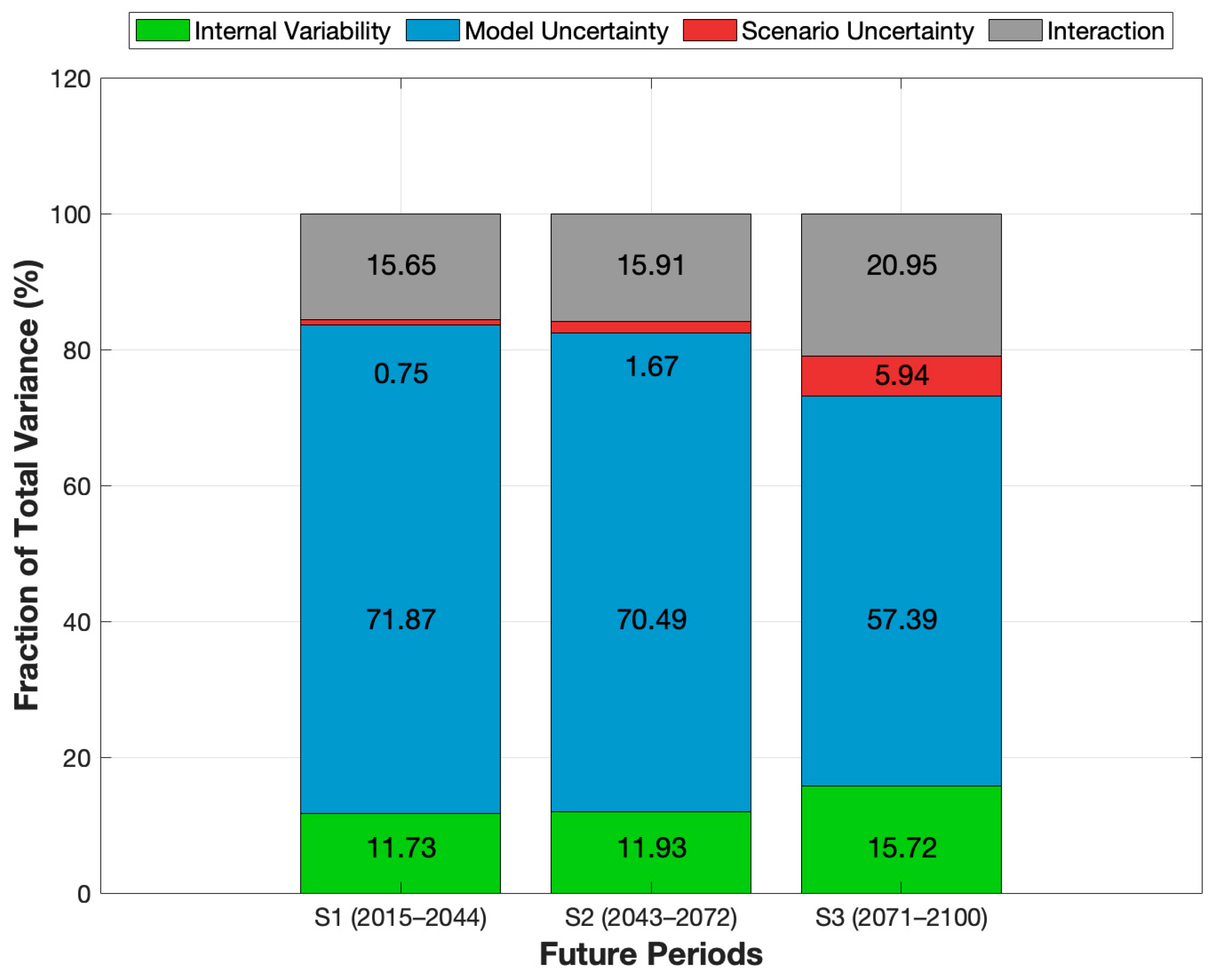
3.2. Uncertainty Analysis

This analysis evaluates the relative contributions of internal variability, model uncertainty, and scenario uncertainty to total uncertainty in climate change projections across three future time periods (Figure 4 and Figure 5). Figure 4 shows the results in a boxplot of different uncertainty sources for 615 sites over three future periods: S1 (2015–2044), S2 (2043–2072), and S3 (2071–2100). Model uncertainty is a predominant factor across all time horizons, consistently representing approximately 60–70% of the total variance. The median values of model uncertainty are approximately 69.4% in S1, 68.3% in S2, and then declining to 55.9% in S3.

As shown in Figure 4a, in the near-term (S1), the interaction effect is the second largest contributor (16.9%), followed by internal volatility (12.7%). During this period, scenario uncertainty remains minimal (less than 1%). This trend typically continues throughout the mid-term period (S2), as illustrated in Figure 4b. The long-term period (S3) depicted in Figure 4c illustrates a substantial transformation. Although model uncertainty continues to be the primary factor, its relative significance decreases over time. In contrast, scenario uncertainty exhibits a marked increase of 6.3%, indicating that the choice of emission pathways is becoming critical in long-term climate forecasts. Additionally, the internal variability and interaction effects rise to 16.5% and 21.4%, respectively.

This analysis underscores several critical observations: in the short-term (S1), model uncertainty emerges as the predominant and most widespread source of uncertainty, underscoring the necessity for ongoing advancements in climate modeling; in the medium-term (S2) and long-term (S3), scenario uncertainty assumes a progressively significant role, emphasizing the importance of delineating future emissions trajectories; furthermore, a systematic review of the evolving contributions of these uncertainties is anticipated to gain importance for the interpretation of climate projections, the direction of research priorities, the formulation of policy decisions, and, ultimately, the enhancement of the reliability of long-term climate assessments.

Figure 5 illustrates the proportional contributions of internal variability, model uncertainty, scenario uncertainty, and their interactions with the overall variance of projected climate change across three distinct future periods (S1, S2, and S3). In the first period (S1), model uncertainty accounts for the largest share at 71.87%, followed by the interaction term at 15.65%, internal variability at 11.73%, and scenario uncertainty at 0.75%. A comparable trend is evident in the second period (S2), where model uncertainty constitutes 70.49%, interactions represent 15.91%, internal variability is at 11.93%, and scenario uncertainty rises to 1.67%. In the third period (S3), model uncertainty declines to 57.39%, while the contributions from the other factors increase, with internal variability at 15.72%, scenario uncertainty at 5.94%, and interactions at 20.96%.

These findings underscore the temporal fluctuations in the primary sources of uncertainty. Model uncertainty consistently emerges as the predominant factor across all timeframes, emphasizing the necessity for advancements in climate modeling and the utilization of multi-model ensembles. Additionally, the increase in scenario uncertainty in the long-term (S3) underscores the significant impact of future emission trajectories. This shifting landscape of uncertainty indicates that enhancing climate modeling, refining emissions scenarios, and deepening our comprehension of internal variability are critical for bolstering the reliability of long-term climate projections.

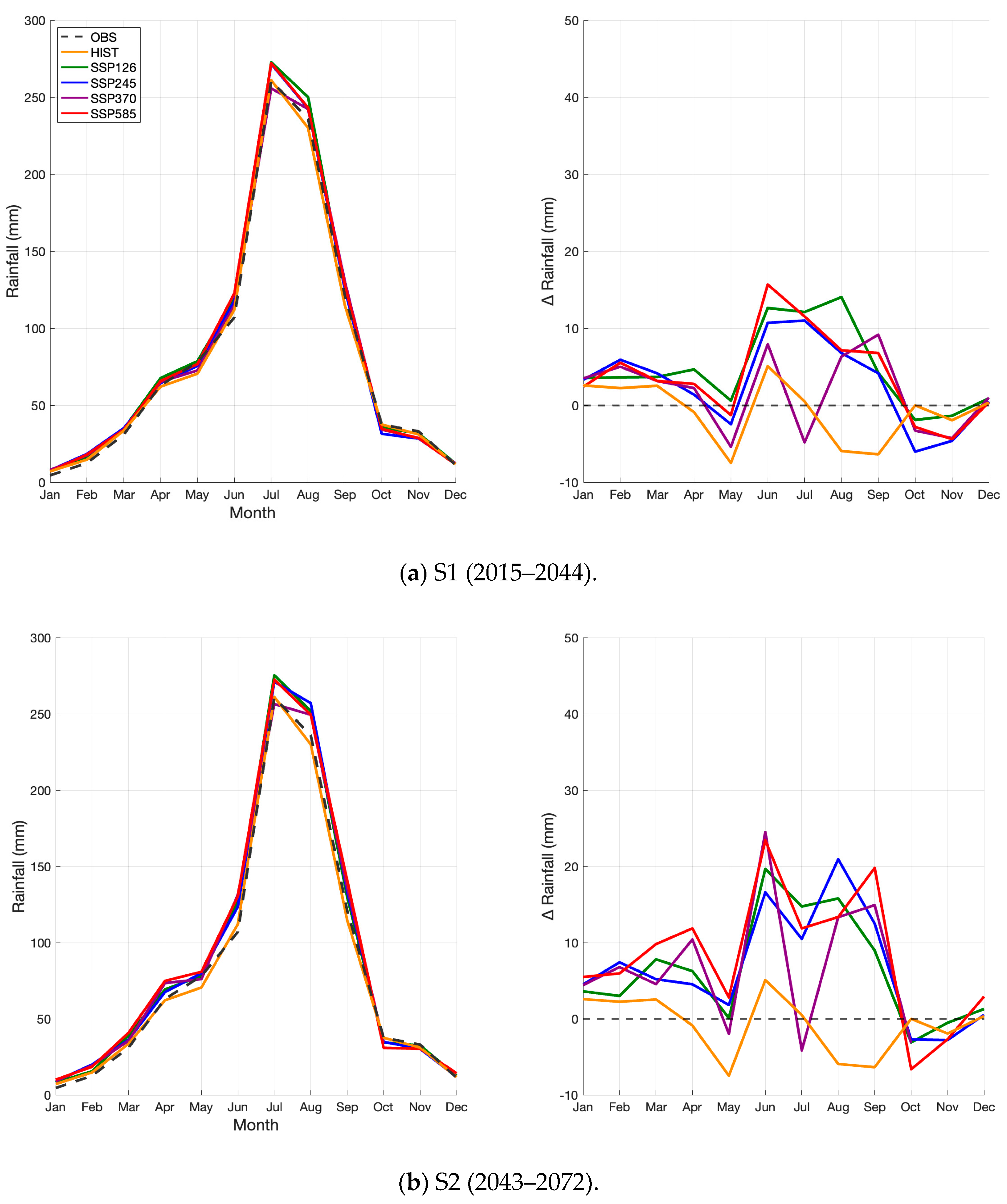
3.3. Future Changes for Monthly and Annual Rainfall

Figure 6a–c illustrates the variations in monthly precipitation across three future projection periods (S1, S2, and S3). Each figure presents the median value of monthly precipitation from 615 observations, utilizing observed data (OBS), historical simulations (HIST), and four distinct scenarios (SSP126, SSP245, SSP370, and SSP585). The figures are organized into two subplots: the left subplot displays the absolute precipitation values, while the right subplot depicts the differences in precipitation (ΔRainfall) relative to the observed values.

A comparison of the actual observations, represented by the black dashed line, with the historical simulations, indicated by the orange solid line, reveals that the values for the months from January to March and June to July surpass the observed measurements. Conversely, the values for the remaining months fall below the observed figures. The discrepancies observed are predominantly within a range of 10 mm, thereby affirming that the climate modeling ensemble data provide a reasonable simulation of the characteristics of the current climatic conditions.

In Figure 6a(S1), all four SSP scenarios demonstrated moderate increases compared to the observed (OBS) and historical (HIST) data, with the most pronounced growth occurring in the peak months of June and July. Among them, SSP585, representing the highest emission scenario, exceeded the historical baseline by roughly 15 mm. Overall, a declining pattern was evident in May as well as from October to December, whereas the other months showed an upward trend, with increases ranging between 5 and 15 mm. Figure 6b(S2) highlights significant differences among the scenarios in the mid-century projections. Notably, SSP370 and SSP585 exhibit an increase of around 25 mm in June, while SSP245 shows a rise of 20 mm in August. Overall, the projected increases during this period were more substantial compared to those observed in the S1 period. Figure 6c(S3) shows that end-of-century projections under the SSP585 scenario reveal a notable rise, exceeding 37 mm in June and 40 mm in September. Similarly, the SSP245 scenario indicates an increase of 35 mm in July, while the other scenarios also display increases of 20 mm or more. Overall, these projections represent the most pronounced changes among the three evaluated time periods.

The data reveal a clear progression from moderate changes in scenario S1 to more pronounced anomalies in scenario S2, culminating in substantial intensification by the end of the century under the high-emission scenario, S3. Among these, the SSP585 scenario consistently shows the largest deviations from historical averages, with increases exceeding 40 mm during peak months in some cases. These results highlight the sensitivity of monthly precipitation patterns to rising greenhouse gas concentrations and emphasize the pressing need for proactive adaptation strategies, particularly in the areas of water infrastructure and flood management.

Figure 7 presents the distribution of annual mean precipitation as depicted by boxplots for four SSP scenarios (SSP126, SSP245, SSP370, SSP585) across three future projection periods (S1, S2, S3). The observed (OBS) median precipitation of 1158.2 mm and historical (HIST) median of 1142.6 mm serve as reference benchmarks. Analysis of the medians reveals a consistent upward trend in annual precipitation across all scenarios and time periods compared to the observed values.

In the near-term period (S1), median annual precipitation increases range from +52.0 mm (SSP370) to +94.0 mm (SSP126), signaling moderate changes. By the mid-term (S2), the differences intensify, with increases between +111.0 mm (SSP370) and +149.6 mm (SSP585), reflecting stronger radiative forcing effects under higher-emission scenarios. In the far-term period (S3), the increases become even more pronounced, particularly under SSP585, which shows a peak median increase of +261.5 mm above the observed baseline. SSP245 and SSP370 also reflect substantial increases of approximately +179 mm each, while SSP126, although more contained, still indicates a rise of +134.7 mm. The expanded interquartile ranges, particularly in SSP370 and SSP585 during the S2 and S3 periods, point to heightened variability in annual precipitation under higher greenhouse gas concentrations. This not only suggests that total precipitation will increase, but also that year-to-year variability may also become more pronounced, posing greater challenges for water resource and infrastructure management.

3.4. Future Rainfall Quantile Changes

Figure 8a shows the median and interquartile range (Q1, Q3) of precipitation quantile estimates for both the observed (OBS) and historical (HIST) periods, particularly for different return periods ranging from 2 to 500 years. To evaluate the consistency between these two datasets, we calculated the median difference ($\mathrm{HIST}-\mathrm{OBS}$) across the specified return periods. For shorter return periods (2–3 years), the HIST values are marginally lower than the OBS values, with differences ranging from −0.4 to −1.1 mm. At the 10-year return period, the difference is nearly negligible at −0.05 mm, and it remains minimal (approximately ±0.1 mm) for the 20- and 30-year return periods. However, for return periods of 50 years and longer, the HIST values consistently surpass the OBS values by approximately +2 mm, with the discrepancy increasing to about +5 mm at the 200- and 500-year return periods. Overall, these modest variations—within ±5 mm—indicate a significant degree of consistency between the OBS and HIST rainfall estimates.

Figure 8b–d presents the findings related to the estimation of rainfall quantiles for each return period, illustrating the rate of change in the future period in comparison to the HIST. Figure 8b illustrates the near-term projections (S1: 2015–2044) for the median rainfall quantiles across various climate scenarios. Under the SSP126 scenario, the median values exhibit a moderate decline, decreasing from approximately 7.36 at the shortest return period to around 5.66 at the longest return period, indicating a gradual reduction in rainfall quantiles as the frequency of events diminishes. In contrast, the SSP245 scenario demonstrates relatively stable median values, ranging from approximately 7.03 to 7.27. Conversely, the SSP370 scenario reveals a significant decrease, with median values dropping from approximately 6.12 to 2.08. The SSP585 scenario presents a more variable trend, beginning at approximately 8.02, reaching a peak of nearly 9.87 in the mid-range, and ultimately stabilizing around 8.59 at the highest return periods. These near-term findings suggest that while the SSP126 and SSP245 scenarios experience relatively modest changes in rainfall quantiles, the SSP370 and SSP585 scenarios are associated with more substantial alterations, particularly at longer return periods.

Figure 8c illustrates the mid-term projections for the period S2: 2043–2072. In the case of SSP126, the median change ratios increase from approximately 7.70, reaching a peak of about 9.17, before declining to approximately 6.78 at the longest return period. This pattern indicates a modest increase in the frequency of events, which diminishes as the rarity of events increases. Conversely, SSP245 demonstrates higher median values overall, beginning at approximately 12.07, peaking at around 12.57, and subsequently decreasing to about 8.52. SSP370 exhibits intermediate characteristics, with medians starting at approximately 10.52, experiencing a slight peak in the mid-range, and ultimately declining to around 7.87. In contrast, SSP585 consistently records the highest median values, ranging from approximately 16.70 to 9.59. These findings suggest that, in the mid-term, the magnitude of changes in rainfall quantiles is most significant under SSP585, while SSP126 shows the least variation.

Figure 8d presents projections for the far-term period (S3: 2071–2100). Under the Shared Socioeconomic Pathway (SSP) 126 scenario, the median values exhibit a significant reduction, decreasing from approximately 11.10 for the shortest return period to around 4.53 for the longest return period, indicating a substantial attenuation of projected changes in extreme events. In the SSP245 scenario, median values decline from roughly 17.46 to 6.69, while in the SSP370 scenario, they decrease from about 19.02 to 9.81. The SSP585 scenario, which corresponds to the highest emissions trajectory, demonstrates the most pronounced change ratios, with median values beginning at approximately 27.72 and falling to about 10.67. Across all scenarios, the consistent downward trend in median values with increasing return periods suggests that, although more frequent events exhibit relatively larger changes, the magnitude of these alterations diminishes for events that are exceedingly rare.

The analyses presented in Figure 8b–d collectively illustrate a distinct temporal progression in the projected changes in rainfall quantiles. In the short-term (S1), the alterations are relatively minor, with only slight variations observed across different scenarios. In the medium-term (S2), these differences become more pronounced, particularly for the SSP585 scenario, which consistently demonstrates the highest ratios of change. By the long-term (S3), the divergence among scenarios becomes significant, with SSP585 and SSP370 indicating markedly greater changes in comparison to SSP126 and SSP245. This comprehensive analysis emphasizes the critical role of emissions trajectories in shaping future patterns of extreme precipitation, revealing an increase in uncertainty and scenario divergence as the return periods and time horizons extend. Such insights are vital for effective hydrological risk assessments and the formulation of adaptation strategies.

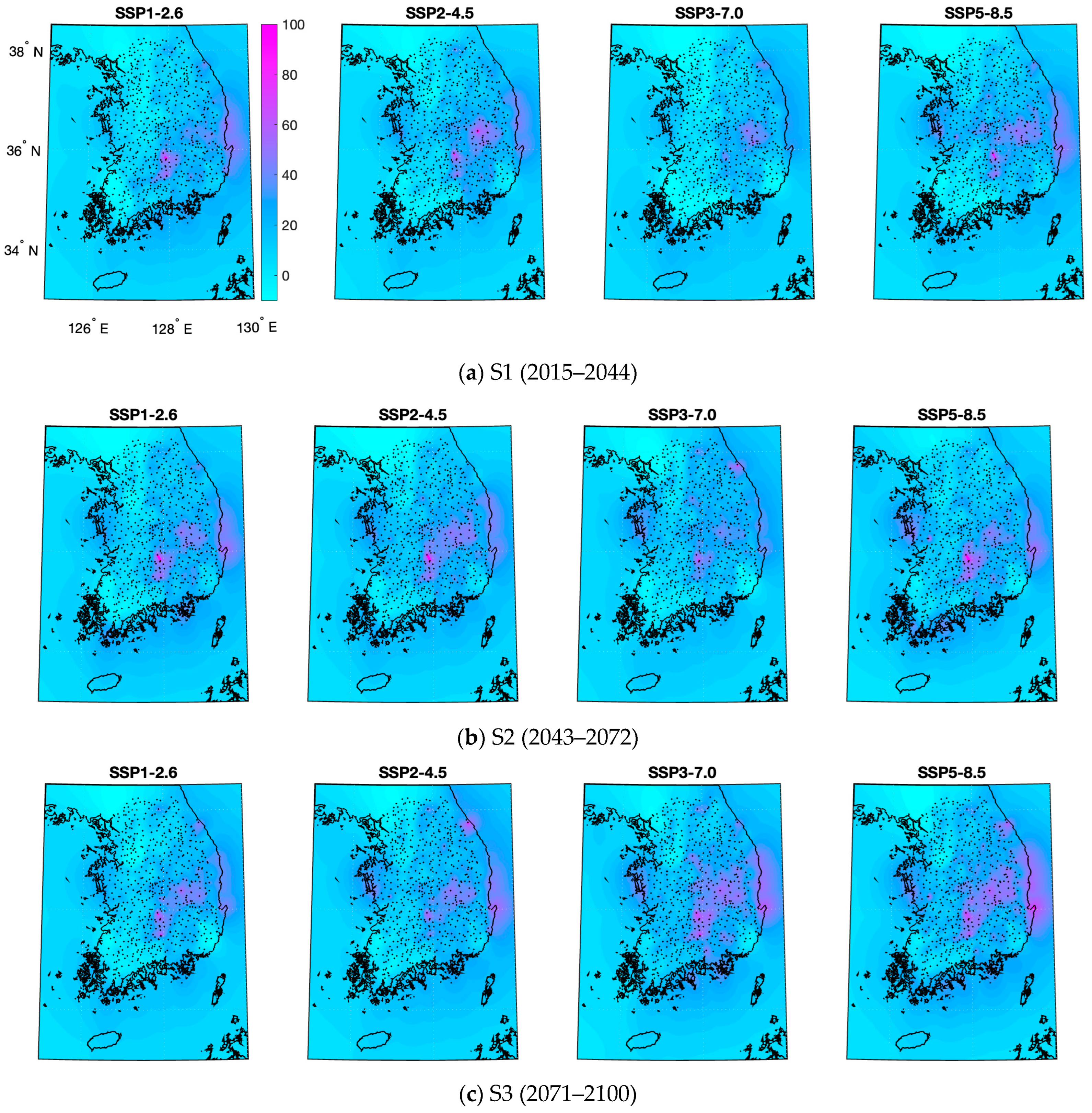
3.5. Spatial Analysis of Rainfall Data

The series of maps in Figure 9 illustrates the projected spatial distributions of precipitation changes across South Korea for three future period, S1 (2015–2044), S2 (2043–2072), and S3 (2071–2100), under four SSP scenarios representing different levels of greenhouse gas emissions and socioeconomic development.

During the near-term (S1) period, all scenarios (SSP126, SSP245, SSP370, and SSP585) exhibited similar spatial patterns of precipitation increases, primarily concentrated in the central and southern regions of Korea. Notably, the SSP245 and SSP585 scenarios projected precipitation increases of approximately 40%, with these increases occurring extensively from the east coast to the central inland regions. In the mid-term period (S2), distinct spatial patterns of precipitation changes emerged across the scenarios. The SSP126 and SSP370 scenarios indicated precipitation increases along the east coast and central regions, while the SSP585 scenario showed a relative decrease compared to the S1 period. The SSP245 scenario exhibited both increases and decreases across different regions while generally maintaining patterns similar to the previous period. The far-term (S3) period demonstrated more pronounced increasing trends across all scenarios. Under SSP585, substantial portions of the country, particularly the central inland and eastern coastal regions, showed projected rainfall increases exceeding 40%. The SSP370 scenario exhibited a notably broader spectrum of increases in comparison to earlier periods, while the low-emission scenarios (SSP126 and SSP245) preserved a spatial distribution akin to that identified during the S2 period.

The consistency in the spatial patterns of change over time was validated using a multi-model ensemble analysis of frequency analysis results from 23 GCMs, providing the average projected changes across all models. These spatial patterns of precipitation change carry significant implications for water resource management and flood risk assessment in Korea. The projected precipitation increases in central and southern regions suggest potential increases in the frequency and intensity of heavy rainfall events, with corresponding elevated flood risks. The variation in magnitude and spatial extent of changes across scenarios underscores the influence of greenhouse gas emission pathways on Korea’s future hydrological landscape. These findings emphasize the necessity for regional adaptation strategies that account for spatial variability in projected precipitation changes, enabling the development of robust targeted approaches to water resource management and flood risk mitigation customized to regional characteristics and vulnerabilities across Korea.

4. Discussion

This study presents a comprehensive assessment of projected precipitation changes across South Korea under various climate change scenarios, employing bias-corrected projections from multiple GCMs. The research framework integrates SQM for bias correction with a multi-model ensemble approach incorporating 23 GCMs, establishing a robust foundation for analyzing climate projections.

The verification of HIST demonstrated the effectiveness of the SQM bias correction method, with RMSE reductions ranging from 63.0% to 85.3% across all GCMs, as well as notable improvements in Pbias (average reduction of 93.6%) and R² (average increase of 0.73). These results align with previous studies [46,51] which reported similar bias reduction magnitudes using quantile mapping approaches. The minor discrepancies observed with previous studies are likely due to the variation in spatial scale, GCM selection, and observational datasets used for bias correction. Nevertheless, the biases of all of the GCMs showed significantly improved results, highlighting the effectiveness of the SQM method in applying bias correction. This study integrates data from 615 regions across South Korea to enhance the accuracy of future climate projections, providing a more robust foundation for water resource planning and management.

The uncertainty analysis identified distinct temporal patterns regarding the contributions of various sources of uncertainty. In the near-term (S1) and mid-term (S2) periods, model uncertainty was the predominant factor, representing approximately 71.87% and 70.49% of the total variance, respectively. In contrast, interaction effects and internal variability contributed smaller proportions, while scenario uncertainty remained negligible, accounting for less than 1% in S1 and 1.67% in S2. These results corroborate the findings of Hawkins and Sutton [52] and Yip et al. [53], who noted the predominance of model uncertainty in early- to mid-century climate projections. However, in the far-term period (S3), the relative contribution of model uncertainty decreased to 57.39%, while scenario uncertainty experienced a significant increase to 5.94%. Additionally, the influence of internal variability rose to 15.72%, and interaction terms accounted for 20.96%. This increasing significance of scenario uncertainty in the far-term underscores the growing impact of emission trajectories on long-term climate projections.

This temporal progression of uncertainty is consistent with prior research [54] which highlighted the difficulties in differentiating anthropogenic signals from natural variability in near-term projections and emphasized the escalating importance of emissions scenarios for far-term projections. These findings underscore the necessity for ongoing advancements in climate modeling to mitigate model uncertainty, the refinement of emissions pathways to diminish scenario uncertainty, and further investigation into internal variability and interaction effects to enhance the reliability of long-term climate assessments.

The analysis of monthly precipitation revealed clear temporal progression from moderate changes in the near-term (S1) to more pronounced anomalies in the mid-term (S2), culminating in substantial increases by the end of the century (S3), particularly under the high-emission scenario, SSP585. Increases exceeding 40 mm during peak months underscore the sensitivity of precipitation patterns to rising greenhouse gas concentrations. In addition, annual mean precipitation showed a consistent upward trend across all scenarios and time periods, with increases becoming notably more pronounced over time. Median annual precipitation increased moderately in the near-term, significantly intensified by the mid-term, and reached peak median increases of up to +261.5 mm under SSP585 by the far-term. Additionally, expanded interquartile ranges indicated greater year-to-year variability in precipitation under high greenhouse gas concentration scenarios, highlighting increasing challenges for water resource planning and infrastructure management.

The analysis of future rainfall quantiles revealed progressively increasing changes across the three time periods, with particularly pronounced changes under higher-emission scenarios. This finding corroborates results from previous regional studies [55,56] which also emphasized greater precipitation changes under high-emission scenarios. The spatial analysis identified significant regional variations, with consistent increases in precipitation projected for the central and southern regions of South Korea, especially along the east coast. Similar regional variability has been reported in previous studies [57,58,59], attributing the variations to localized atmospheric circulation patterns, the Asian summer monsoon, and topographic effects.

This extensive analysis highlights the necessity for specific climate adaptation and mitigation strategies in South Korea, particularly in light of anticipated regional increases in precipitation, especially in the central and southern areas along the east coast. Despite the presence of inherent uncertainties and variability, the comprehensive multi-model framework utilized in this study effectively enables us to perform a bias correction and uncertainty assessment, demonstrating strong alignment with previous research outcomes. Ongoing improvements in climate modeling and emissions scenarios are essential for bolstering the reliability of long-term climate projections and guiding sustainable water resource management practices.

5. Conclusions

This study investigates changes in extreme rainfall patterns in South Korea by utilizing the CMIP6 climate change scenarios. The analysis incorporated data from 23 GCMs and employed SQM bias correction based on observations from 615 sites across the country. The bias-corrected datasets were regionalized into 26 clusters, followed by a regional frequency analysis. Furthermore, a multi-model ensemble approach was employed to evaluate quantitative changes over the simulated timeframes. The principal findings obtained from this study are as follows:

(1)

HIST data have validated the efficacy of the SQM bias correction technique, which has been shown to significantly mitigate model bias. Notable reductions in RMSE and Pbias and enhancements in R² values underscore the robustness of the SQM method for the correction of climate models.

(2)

Model uncertainty has been identified as a significant factor influencing climate projections in both the short- and mid-term. Furthermore, in the long-term, scenario uncertainty and internal variability have emerged as increasingly important contributors to the overall uncertainty associated with climate forecasts. This shift underscores the growing significance of emission scenarios in the realm of long-term climate change projections.

(3)

An analysis of monthly precipitation patterns revealed progressively larger increases, transitioning from moderate near-term changes to substantial anomalies in the far-term period, particularly under the high-emission scenario (SSP585). The significant increases in monthly precipitation underscore the sensitivity of precipitation patterns to elevated greenhouse gas concentrations.

(4)

Annual precipitation has demonstrated a consistent upward trend across all scenarios and future timeframes, with the most significant increases occurring under SSP585 as the century draws to a close. Furthermore, the observed rise in year-to-year variability presents future challenges for the management of water resources.

(5)

Projections indicate that future rainfall quantiles are expected to increase progressively, particularly under high-emission scenarios. Significant regional variability has been observed, especially in central and southern South Korea, as well as along the eastern coastline. These spatial discrepancies reflect the influences of atmospheric circulation, the Asian summer monsoon, and local topographical features.

This study highlights the necessity of addressing model uncertainties, refining emission scenarios, and comprehending internal climate variability. These results offer essential guidance for climate adaptation planning in South Korea, especially in water resource management and flood risk mitigation. The clear link between emission scenarios and projected rainfall intensification underscores the critical role of climate mitigation strategies. Future research should focus on enhancing spatial resolution by using advanced downscaling techniques and integrating hydrological models with socioeconomic risk assessments. Overall, this study provides a strong scientific foundation to support the development of resilient water management strategies and infrastructure systems across the Korean Peninsula.

References

1. de Vries, I.; Sippel, S.; Zeder, J.; Fischer, E.; Knutti, R. Increasing extreme precipitation variability plays a key role in future record-shattering event probability. Commun. Earth Environ. 2024, 5, 482. [Google Scholar] [CrossRef] [PubMed]
2. Fowler, H.J.; Lenderink, G.; Prein, A.F.; Westra, S.; Allan, R.P.; Ban, N.; Barbero, R.; Berg, P.; Blenkinsop, S.; Do, H.X.; et al. Anthropogenic intensification of short-duration rainfall extremes. Nat. Rev. Earth Environ. 2021, 2, 107–122. [Google Scholar] [CrossRef]
3. Jung, I.W.; Bae, D.H.; Lee, B.J. Possible change in Korean streamflow seasonality based on multi-model climate projections. Hydrol. Process. 2013, 27, 1033–1045. [Google Scholar] [CrossRef]
4. Cha, D.H.; Lee, D.K.; Jin, C.S.; Kim, G.; Choi, Y.; Suh, M.-S.; Ahn, J.-B.; Hong, S.-Y.; Min, S.-K.; Park, S.-C.; et al. Future changes in summer precipitation in regional climate simulations over the Korean Peninsula forced by multi-RCP scenarios of HadGEM2-AO. Asia-Pac. J. Atmos. Sci. 2016, 52, 139–149. [Google Scholar] [CrossRef]
5. Park, C.; Son, S.-W.; Kim, H.; Ham, Y.-G.; Kim, J.; Cha, D.-H.; Chang, E.-C.; Lee, G.W.; Kug, J.-S.; Lee, W.-S.; et al. Record-breaking summer rainfall in South Korea in 2020: Synoptic characteristics and the role of large-scale circulations. Mon. Weather Rev. 2021, 149, 3085–3100. [Google Scholar] [CrossRef]
6. Kim, S.; Park, J.H.; Kug, J.S. Tropical origins of the record-breaking 2020 summer rainfall extremes in East Asia. Sci. Rep. 2022, 12, 5366. [Google Scholar] [CrossRef] [PubMed]
7. Park, C.; Min, S.K.; Lee, D.; Cha, D.-H.; Suh, M.-S.; Kang, H.-S.; Hong, S.-Y.; Lee, D.-K.; Baek, H.-J.; Boo, K.-O.; et al. Evaluation of multiple regional climate models for summer climate extremes over East Asia. Clim. Dyn. 2016, 46, 2469–2486. [Google Scholar] [CrossRef]
8. Salas, J.D.; Obeysekera, J.; Vogel, R.M. Techniques for assessing water infrastructure for nonstationary extreme events: A review. Hydrol. Sci. J. 2018, 63, 325–352. [Google Scholar] [CrossRef]
9. Cheng, L.; AghaKouchak, A. Nonstationary precipitation intensity–duration–frequency curves for infrastructure design in a changing climate. Sci. Rep. 2014, 4, 7093. [Google Scholar] [CrossRef]
10. Lim, G.-K.; Kim, B.-S.; Lee, B.-H.; Jeung, S.-J. Effect of climate change on annual precipitation in Korea using data screening techniques and climate change scenarios. Atmosphere 2020, 11, 1027. [Google Scholar] [CrossRef]
11. Wang, G.; Wang, D.; Trenberth, K.E.; Erfanian, A.; Yu, M.; Bosilovich, M.G.; Parr, D.T. The peak structure and future changes of the relationships between extreme precipitation and temperature. Nat. Clim. Chang. 2017, 7, 268–274. [Google Scholar] [CrossRef]
12. Sillmann, J.; Kharin, V.V.; Zwiers, F.W.; Zhang, X.; Bronaugh, D. Climate extremes indices in the CMIP5 multimodel ensemble: Part 2. Future climate projections. J. Geophys. Res. Atmos. 2013, 118, 2473–2493. [Google Scholar] [CrossRef]
13. Sperber, K.R.; Annamalai, H.; Kang, I.-S.; Kitoh, A.; Moise, A.; Turner, A.; Wang, B.; Zhou, T. The Asian summer monsoon: An intercomparison of CMIP5 vs. CMIP3 simulations of the late 20th century. Clim. Dyn. 2013, 41, 2711–2744. [Google Scholar] [CrossRef]
14. Wang, B.; Liu, J.; Kim, H.-J.; Webster, P.J.; Yim, S.-Y. Recent change of the global monsoon precipitation (1979–2008). Clim. Dyn. 2012, 39, 1123–1135. [Google Scholar] [CrossRef]
15. Eyring, V.; Bony, S.; Meehl, G.A.; Senior, C.A.; Stevens, B.; Stouffer, R.J.; Taylor, K.E. Overview of the Coupled Model Intercomparison Project Phase 6 (CMIP6) experimental design and organization. Geosci. Model Dev. 2016, 9, 1937–1958. [Google Scholar] [CrossRef]
16. Adelodun, B.; Ahmad, M.J.; Odey, G.; Adeyi, Q.; Choi, K.S. Performance-based evaluation of CMIP5 and CMIP6 global climate models and their multi-model ensembles to simulate and project seasonal and annual climate variables in the Chungcheong region of South Korea. Atmosphere 2023, 14, 1569. [Google Scholar] [CrossRef]
17. Shin, Y.; Shin, Y.; Hong, J.; Kim, M.-K.; Byun, Y.-H.; Boo, K.-O.; Chung, I.-U.; Park, D.-S.R.; Park, J.-S. Future Projections and Uncertainty Assessment of Precipitation Extremes in the Korean Peninsula from the CMIP6 Ensemble with a Statistical Framework. Atmosphere 2021, 12, 97. [Google Scholar] [CrossRef]
18. Chen, Z.; Zhou, T.; Zhang, L.; Chen, X.; Zhang, W.; Jiang, J. Global land monsoon precipitation changes in CMIP6 projections. Geophys. Res. Lett. 2020, 47, e2019GL086902. [Google Scholar] [CrossRef]
19. Kim, Y.H.; Min, S.K.; Zhang, X.; Sillmann, J.; Sandstad, M. Evaluation of the CMIP6 multi-model ensemble for climate extreme indices. Weather Clim. Extremes 2020, 29, 100269. [Google Scholar] [CrossRef]
20. Korea Meteorological Administration (KMA). Annual Climatological Report; KMA: Seoul, Republic of Korea, 2023.
21. Beck, H.E.; Zimmermann, N.E.; McVicar, T.R.; Vergopolan, N.; Berg, A.; Wood, E.F. Present and future Köppen–Geiger climate classification maps at 1-km resolution. Sci. Data 2018, 5, 180214. [Google Scholar] [CrossRef]
22. Chough, S.K.; Ree, J.H.; Choi, D.K.; Yoon, S.H. Tectonic and sedimentary evolution of the Korean peninsula: A review and new view. Earth-Sci. Rev. 2000, 52, 175–235. [Google Scholar] [CrossRef]
23. Water Resources Management Information System (WAMIS). Available online: http://www.wamis.go.kr (accessed on 19 March 2025).
24. Bi, D.; Dix, M.; Marsland, S.; O’Farrell, S.; Sullivan, A.; Bodman, R.; Law, R.; Harman, I.; Srbinovsky, J.; Rashid, H.A.; et al. Configuration and spin-up of ACCESS-CM2, the new generation Australian Community Climate and Earth System Simulator coupled model. J. South. Hemisph. Earth Syst. Sci. 2020, 70, 225–251. [Google Scholar] [CrossRef]
25. Ziehn, T.; Chamberlain, M.A.; Law, R.M.; Lenton, A.; Bodman, R.W.; Dix, M.; Stevens, L.; Wang, Y.P.; Srbinovsky, J. The Australian Earth System Model: ACCESS-ESM1.5. J. South. Hemisph. Earth Syst. Sci. 2020, 70, 193–214. [Google Scholar] [CrossRef]
26. Semmler, T.; Danilov, S.; Gierz, P.; Goessling, H.F.; Hegewald, J.; Hinrichs, C.; Koldunov, N.; Khosravi, N.; Mu, L.; Rackow, T.; et al. Simulations for CMIP6 with the AWI Climate Model AWI-CM-1-1. J. Adv. Model. Earth Syst. 2020, 12, e2019MS002009. [Google Scholar] [CrossRef]
27. Wu, T.; Lu, Y.; Fang, Y.; Xin, X.; Li, L.; Li, W.; Jie, W.; Zhang, J.; Liu, Y.; Zhang, L.; et al. The Beijing Climate Center Climate System Model (BCC-CSM): The main progress from CMIP5 to CMIP6. Geosci. Model Dev. 2019, 12, 1573–1600. [Google Scholar] [CrossRef]
28. Swart, N.C.; Cole, J.N.S.; Kharin, V.V.; Lazare, M.; Scinocca, J.F.; Gillett, N.P.; Anstey, J.; Arora, V.; Christian, J.R.; Hanna, S.; et al. The Canadian Earth System Model version 5 (CanESM5.0.3). Geosci. Model Dev. 2019, 12, 4823–4873. [Google Scholar] [CrossRef]
29. Cherchi, A.; Fogli, P.G.; Lovato, T.; Peano, D.; Iovino, D.; Gualdi, S.; Masina, S.; Scoccimarro, E.; Materia, S.; Bellucci, A.; et al. Global mean climate and main patterns of variability in the CMCC-CM2 coupled model. J. Adv. Model. Earth Syst. 2019, 11, 185–209. [Google Scholar] [CrossRef]
30. Lovato, T.; Peano, D.; Butenschön, M.; Materia, S.; Iovino, D.; Scoccimarro, E.; Fogli, P.G.; Cherchi, A.; Bellucci, A.; Gualdi, S.; et al. CMIP6 simulations with the CMCC Earth System Model (CMCC-ESM2). J. Adv. Model. Earth Syst. 2022, 14, e2021MS002814. [Google Scholar] [CrossRef]
31. Wyser, K.; van Noije, T.; Yang, S.; von Hardenberg, J.; O’Donnell, D.; Döscher, R. On the increased climate sensitivity in the EC-Earth model from CMIP5 to CMIP6. Geosci. Model Dev. 2020, 13, 3465–3474. [Google Scholar] [CrossRef]
32. Döscher, R.; Acosta, M.; Alessandri, A.; Anthoni, P.; Arsouze, T.; Bergman, T.; Bernardello, R.; Boussetta, S.; Caron, L.-P.; Carver, G.; et al. The EC-Earth3 Earth system model for the Coupled Model Intercomparison Project 6. Geosci. Model Dev. 2022, 15, 2973–3020. [Google Scholar] [CrossRef]
33. Li, L.; Yu, Y.; Tang, Y.; Lin, P.; Xie, J.; Song, M.; Dong, L.; Zhou, T.; Liu, L.; Wang, L.; et al. The flexible global ocean–atmosphere–land system model grid-point version 3 (fgoals-g3): Description and evaluation. J. Adv. Model. Earth Syst. 2020, 12, e2019MS002012. [Google Scholar] [CrossRef]
34. Held, I.M.; Guo, H.; Adcroft, A.; Dunne, J.P.; Horowitz, L.W.; Krasting, J.; Shevliakova, E.; Winton, M.; Zhao, M.; Bushuk, M.; et al. Structure and performance of GFDL’s CM4.0 climate model. J. Adv. Model. Earth Syst. 2019, 11, 3691–3727. [Google Scholar] [CrossRef]
35. Swapna, P.; Krishnan, R.; Sandeep, N.; Prajeesh, A.G.; Ayantika, D.C.; Manmeet, S.; Vellore, R. Long-term climate simulations using the IITM Earth System Model (IITM-ESMv2) with focus on the South Asian monsoon. J. Adv. Model. Earth Syst. 2018, 10, 1127–1149. [Google Scholar] [CrossRef]
36. Volodin, E.M.; Mortikov, E.V.; Kostrykin, S.V.; Galin, V.Y.; Lykossov, V.N.; Gritsun, A.S.; Diansky, N.A.; Gusev, A.V.; Iakovlev, N.G.; Shestakova, A.A.; et al. Simulation of the modern climate using the INM-CM48 climate model. Russ. J. Numer. Anal. Math. Model. 2018, 33, 367–374. [Google Scholar] [CrossRef]
37. Volodin, E.M.; Mortikov, E.V.; Kostrykin, S.V.; Galin, V.Y.; Lykossov, V.N.; Gritsun, A.S.; Diansky, N.A.; Gusev, A.V.; Iakovlev, N.G. Simulation of the present-day climate with the climate model INMCM5. Clim. Dyn. 2017, 49, 3715–3734. [Google Scholar] [CrossRef]
38. Lurton, T.; Balkanski, Y.; Bastrikov, V.; Bekki, S.; Bopp, L.; Braconnot, P.; Brockmann, P.; Cadule, P.; Contoux, C.; Cozic, A.; et al. Implementation of the CMIP6 forcing data in the IPSL-CM6A-LR model. J. Adv. Model. Earth Syst. 2020, 12, e2019MS001940. [Google Scholar] [CrossRef]
39. Lee, J.; Kim, J.; Sun, M.-A.; Kim, B.-H.; Moon, H.; Sung, H.M.; Kim, J.; Byun, Y.-H. Evaluation of the Korea Meteorological Administration Advanced Community Earth-System model (K-ACE). Asia-Pac. J. Atmos. Sci. 2020, 56, 381–395. [Google Scholar] [CrossRef]
40. Tatebe, H.; Ogura, T.; Nitta, T.; Komuro, Y.; Ogochi, K.; Takemura, T.; Sudo, K.; Sekiguchi, M.; Abe, M.; Saito, F.; et al. Description and basic evaluation of simulated mean state, internal variability, and climate sensitivity in MIROC6. Geosci. Model Dev. 2019, 12, 2727–2765. [Google Scholar] [CrossRef]
41. Gutjahr, O.; Putrasahan, D.; Lohmann, K.; Jungclaus, J.H.; von Storch, J.-S.; Brüggemann, N.; Haak, H.; Stössel, A. Max Planck Institute Earth System Model (MPI-ESM1.2) for the High-Resolution Model Intercomparison Project (HighResMIP). Geosci. Model Dev. 2019, 12, 3241–3281. [Google Scholar] [CrossRef]
42. Mauritsen, T.; Bader, J.; Becker, T.; Behrens, J.; Bittner, M.; Brokopf, R.; Brovkin, V.; Claussen, M.; Crueger, T.; Esch, M.; et al. Developments in the MPI-M Earth System Model version 1.2 (MPI-ESM1.2) and its response to increasing CO2. J. Adv. Model. Earth Syst. 2019, 11, 998–1038. [Google Scholar] [CrossRef]
43. Yukimoto, S.; Kawai, H.; Koshiro, T.; Oshima, N.; Yoshida, K.; Urakawa, S.; Tsujino, H.; Deushi, M.; Tanaka, T.; Hosaka, M.; et al. The Meteorological Research Institute Earth System Model Version 2.0, MRI-ESM2.0: Description and basic evaluation of the physical component. J. Meteorol. Soc. Jpn. Ser. II 2019, 97, 931–965. [Google Scholar] [CrossRef]
44. Seland, Ø.; Bentsen, M.; Olivié, D.; Toniazzo, T.; Gjermundsen, A.; Graff, L.S.; Debernard, J.B.; Gupta, A.K.; He, Y.-C.; Kirkevåg, A.; et al. Overview of the Norwegian Earth System Model (NorESM2) and key climate response of CMIP6 DECK, historical, and scenario simulations. Geosci. Model Dev. 2020, 13, 6165–6200. [Google Scholar] [CrossRef]
45. Lee, W.-L.; Wang, Y.-C.; Shiu, C.-J.; Tsai, I.-C.; Tu, C.-Y.; Lan, Y.-Y.; Chen, J.-P.; Pan, H.-L.; Hsu, H.-H. Taiwan Earth System Model Version 1: Description and evaluation of mean state. Geosci. Model Dev. 2020, 13, 3887–3904. [Google Scholar] [CrossRef]
46. Cho, J.; Jung, I.; Cho, W.; Hwang, S. User-Centered Climate Change Scenarios Technique Development and Application of Korean Peninsula. J. Clim. Chang. Res. 2018, 9, 13–29. [Google Scholar] [CrossRef]
47. Gudmundsson, L.; Bremnes, J.B.; Haugen, J.E.; Engen-Skaugen, T. Technical Note: Downscaling RCM Precipitation to the Station Scale Using Statistical Transformations—A Comparison of Methods. Hydrol. Earth Syst. Sci. 2012, 16, 3383–3390. [Google Scholar] [CrossRef]
48. Cho, J.; Ko, G.; Kim, K.; Oh, C. Climate Change Impacts on Agricultural Drought with Consideration of Uncertainty in CMIP5 Scenarios. Irrig. Drain. 2016, 65, 7–15. [Google Scholar] [CrossRef]
49. Gudmundsson, L. qmap: Statistical Transformations for Post-Processing Climate Model Output, Version 1.0-6. R Package. 2025. Available online: https://cran.r-project.org/web/packages/qmap/ (accessed on 2 February 2025).
50. Ministry of Environment (MOE). Standard Guidelines on Flood Estimation; MOE: Sejong, Republic of Korea, 2019.
51. Cho, J.-P.; Kim, J.-U.; Choi, S.-K.; Hwang, S.; Jung, H. Variability Analysis of Climate Extreme Index Using Downscaled Multi-Models and Grid-Based CMIP5 Climate Change Scenario Data. J. Clim. Chang. Res. 2020, 11, 123–132. [Google Scholar] [CrossRef]
52. Hawkins, E.; Sutton, R. The Potential to Narrow Uncertainty in Regional Climate Predictions. Bull. Am. Meteorol. Soc. 2009, 90, 1095–1108. [Google Scholar] [CrossRef]
53. Yip, S.; Ferro, C.A.T.; Stephenson, D.B.; Hawkins, E. A Simple, Coherent Framework for Partitioning Uncertainty in Climate Predictions. J. Clim. 2011, 24, 4634–4643. [Google Scholar] [CrossRef]
54. Lee, Y.; Shin, Y.; Boo, K.-O.; Park, J.-S. Future Projections and Uncertainty Assessment of Precipitation Extremes in the Korean Peninsula from the CMIP5 Ensemble. Atmos. Sci. Lett. 2020, 21, e954. [Google Scholar] [CrossRef]
55. Noh, S.J.; Lee, G.; Kim, B.; Lee, S.; Jo, J.; Woo, D.K. Climate Change Impact Assessment on Water Resources Management Using a Combined Multi-Model Approach in South Korea. J. Hydrol. Reg. Stud. 2024, 53, 101842. [Google Scholar] [CrossRef]
56. Kim, S.; Joo, K.; Kim, H.; Shin, J.-Y.; Heo, J.-H. Regional Quantile Delta Mapping Method Using Regional Frequency Analysis for Regional Climate Model Precipitation. J. Hydrol. 2021, 596, 125685. [Google Scholar] [CrossRef]
57. Moazzam, M.F.U.; Rahman, G.; Munawar, S.; Farid, N.; Lee, B.G. Spatiotemporal Rainfall Variability and Drought Assessment during Past Five Decades in South Korea Using SPI and SPEI. Atmosphere 2022, 13, 292. [Google Scholar] [CrossRef]
58. Lee, M.; An, H.; Lee, J.; Um, M.-J.; Jung, Y.; Kim, K.; Jung, K.; Kim, S.; Park, D. Spatiotemporal Variability of Regional Rainfall Frequencies in South Korea for Different Periods. Sustainability 2023, 15, 16646. [Google Scholar] [CrossRef]
59. Kim, S.; Seo, M.; Kim, H.; Lee, T.; Kim, G.; Heo, J.-H. Future Changes in Extreme Rainfall Over South Korea: Based on AR6 Climate Scenarios. In Sustainable Design and Eco Technologies for Infrastructure; Ghai, R., Chang, L.M., Sharma, R., Chandrappa, A.K., Eds.; CECAR 2022, Lecture Notes in Civil Engineering; Springer: Singapore, 2024; Volume 441. [Google Scholar] [CrossRef]
Figure 1. Geographical distribution of the study area (shaded in light blue) and the 615 rainfall observation sites (red dots).
Water 17 00894 g001
Figure 2. RMSE, Pbias, and R2 values before (gray) and after (blue) bias correction for 615 points. The boxplot on the right illustrates the distribution of RMSE values across 23 GCMs.
Water 17 00894 g002aWater 17 00894 g002b
Figure 3. Improvement of RMSE, Pbias, and R2 for 23 GCMs based on SQM bias correction method.
Water 17 00894 g003
Figure 4. Boxplot of each uncertainty for each period across 615 sites.
Water 17 00894 g004
Figure 5. Relative contributions of internal variability, model uncertainty, and scenario uncertainty to the total uncertainty in climate change projections across three future periods: S1 (2015–2044), S2 (2043–2072), and S3 (2071–2100). The interaction term represents the uncertainty arising from the interplay between these three sources.
Water 17 00894 g005
Figure 6. Differences in monthly precipitation compared to the observed values for each future period based on the median of 615 sites.
Water 17 00894 g006aWater 17 00894 g006b
Figure 7. Annual mean precipitations across 615 sites for both the observed and projected periods.
Water 17 00894 g007
Figure 8. Rainfall quantiles (OBS and HIST) and future change ratios across the climate change scenarios and future periods (S1, S2, and S3).
Water 17 00894 g008
Figure 9. Spatial distributions of rainfall changes over South Korea for three future time periods: S1 (2015–2044), S2 (2043–2072), and S3 (2071–2100).
Water 17 00894 g009