
Tidal-Driven Water Residence Time in the Bohai and Yellow Seas: The Roles of Different Tidal Constituents


Abstract
1. Introduction
2. Methods
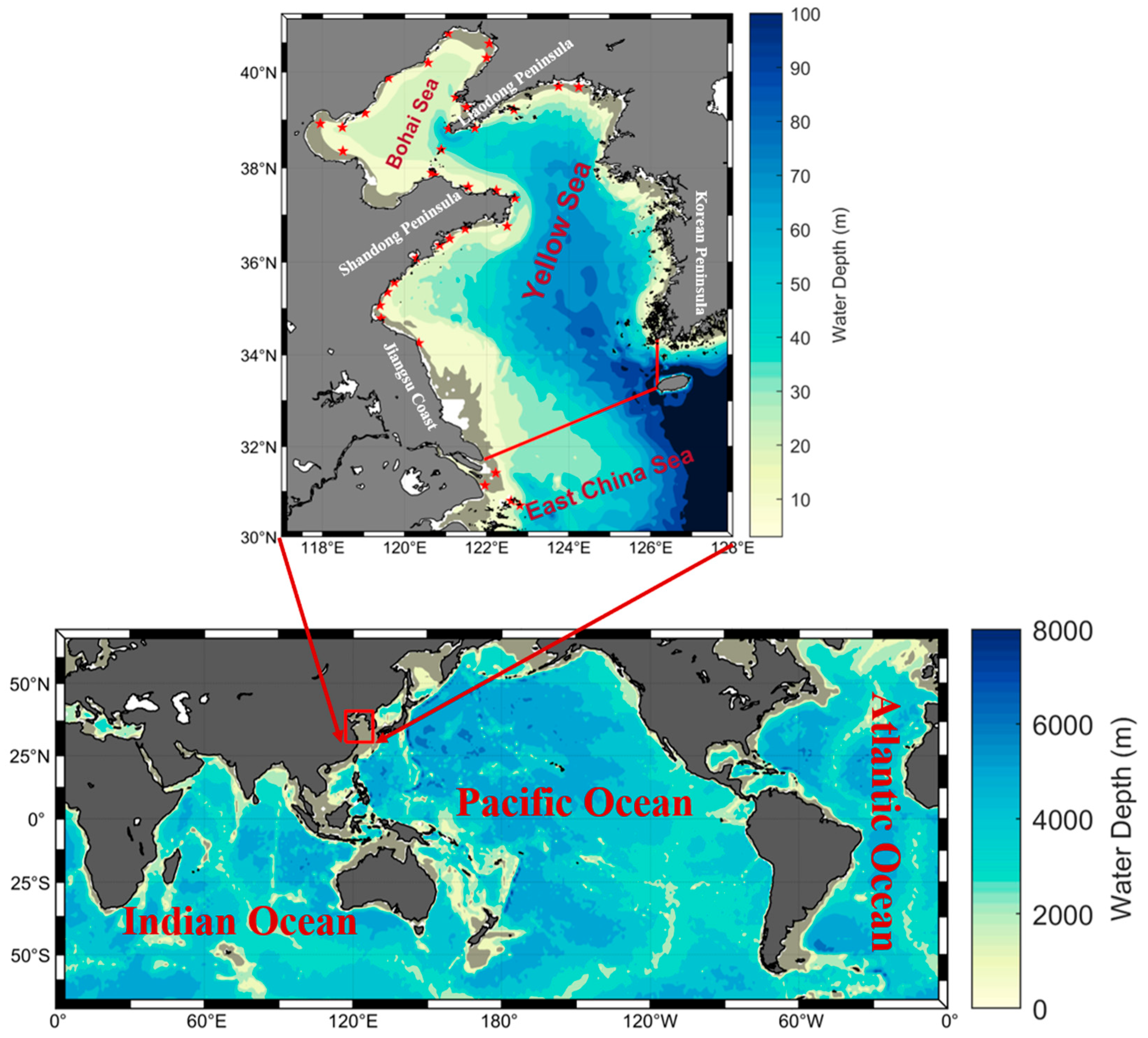
2.1. Study Area
2.2. Tidal Simulation by the MERF Model
2.3. Diagnosis of Water Residence Time
2.4. Numerical Sensitivity Experiments
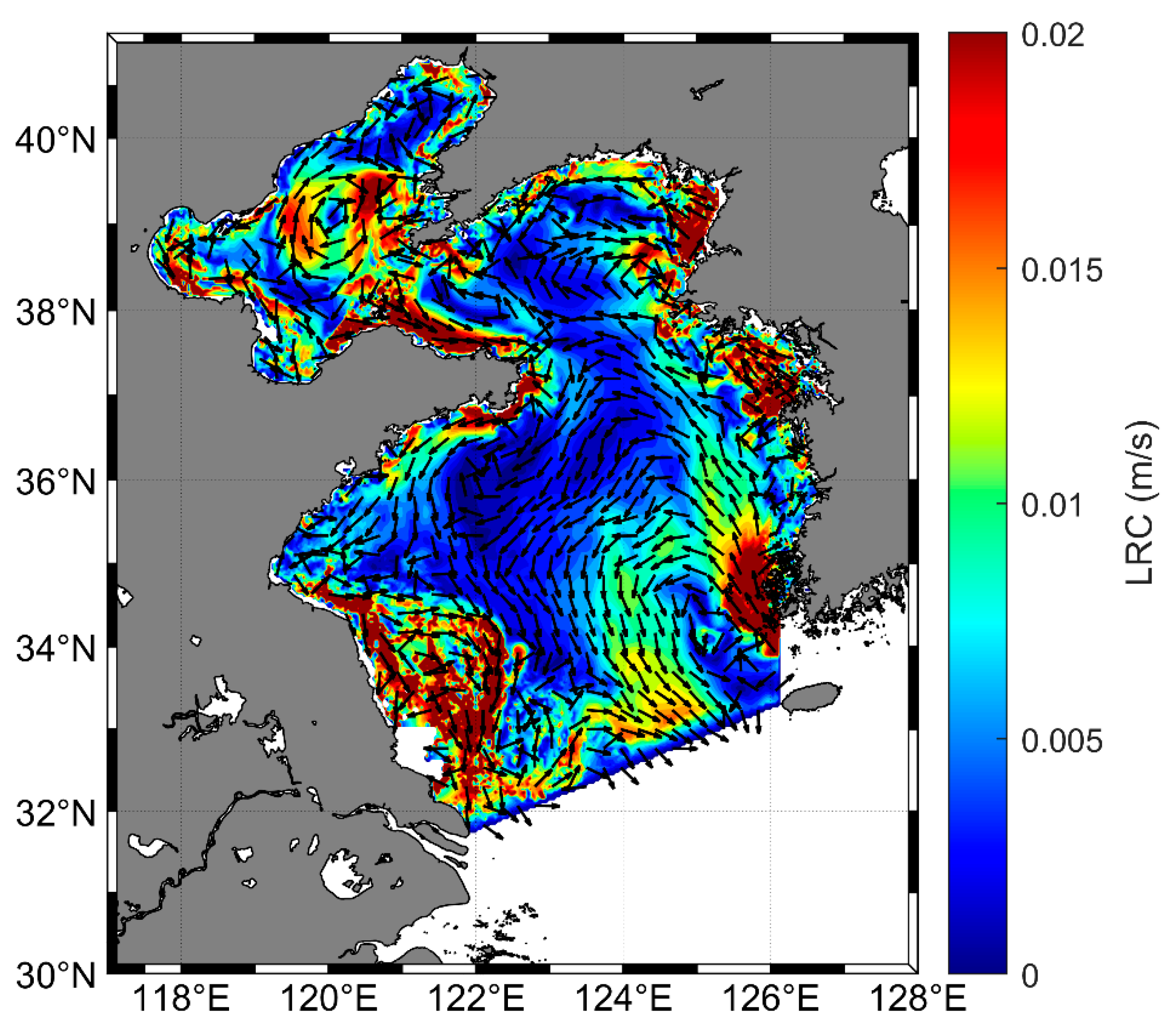
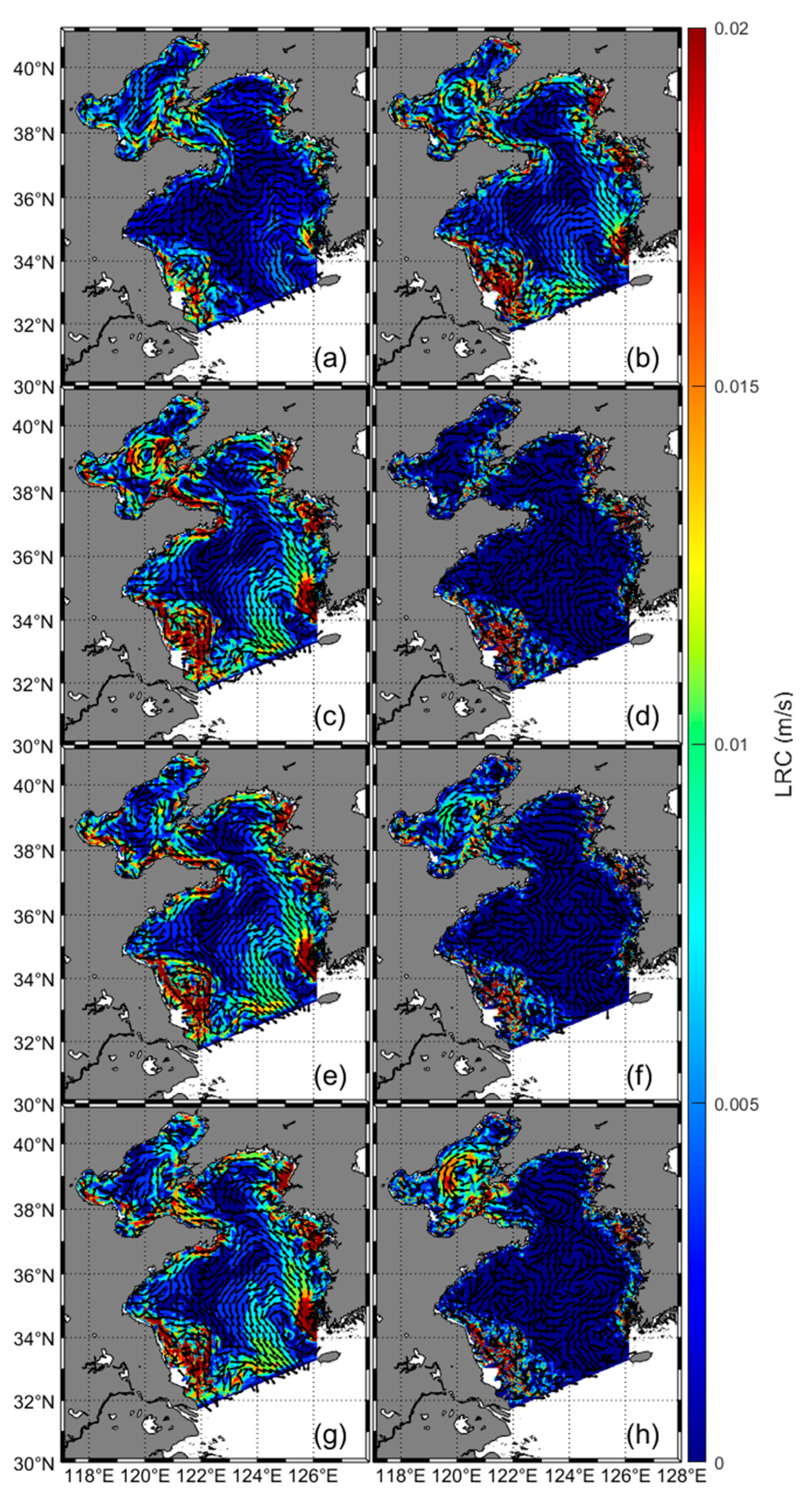
2.5. Lagrangian Residual Currents
3. Results
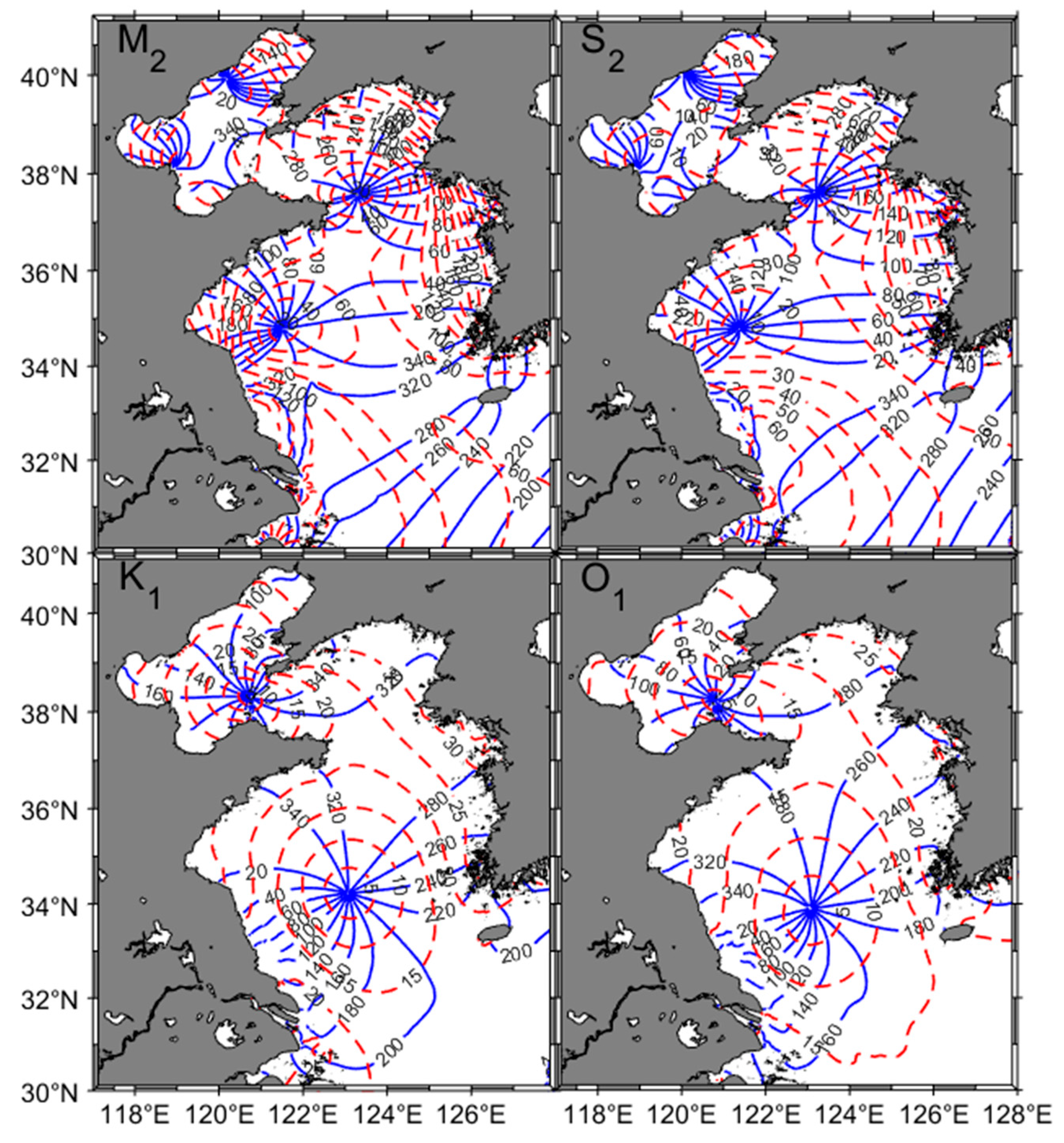
3.1. Validation of the Tidal Simulation
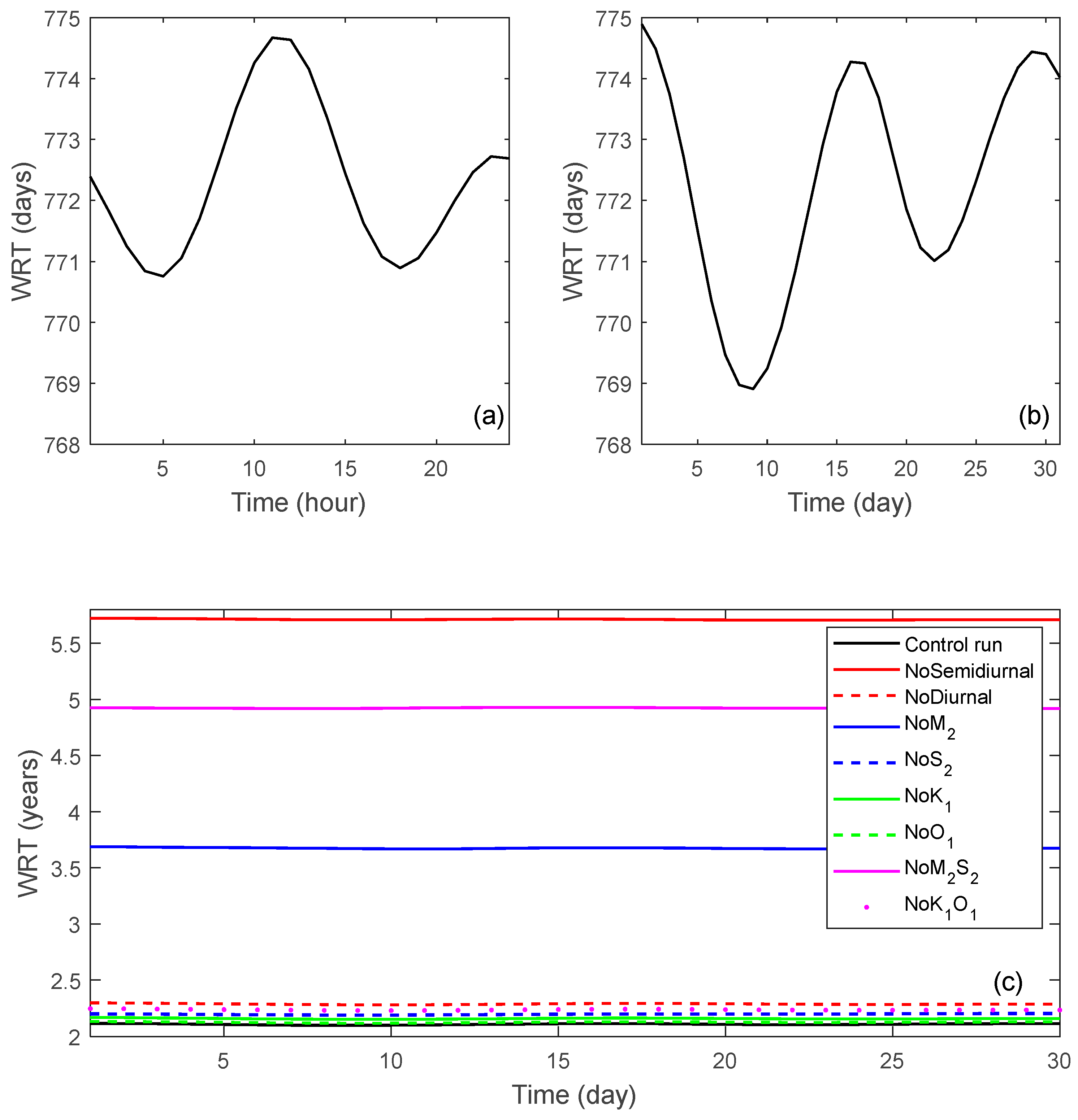
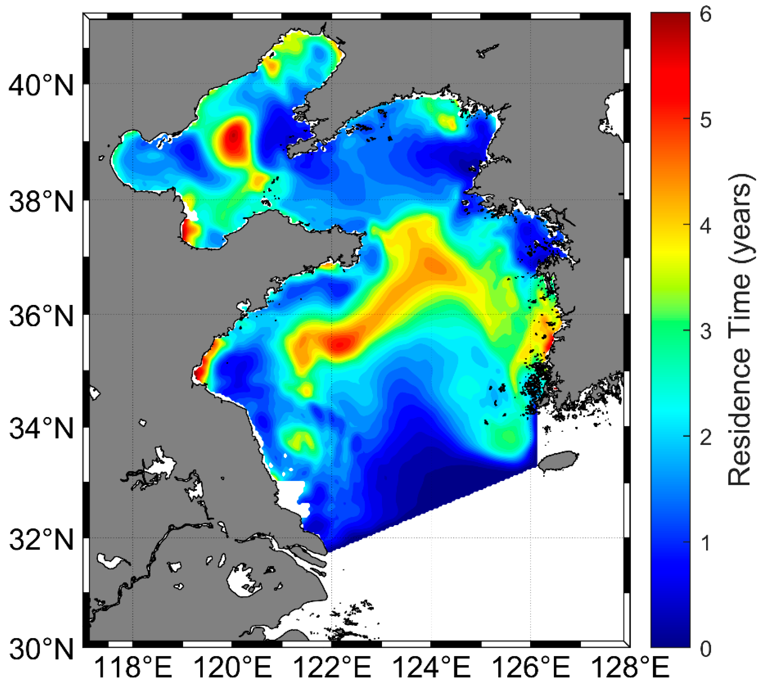
3.2. Tidal-Driven WRT in the BYS
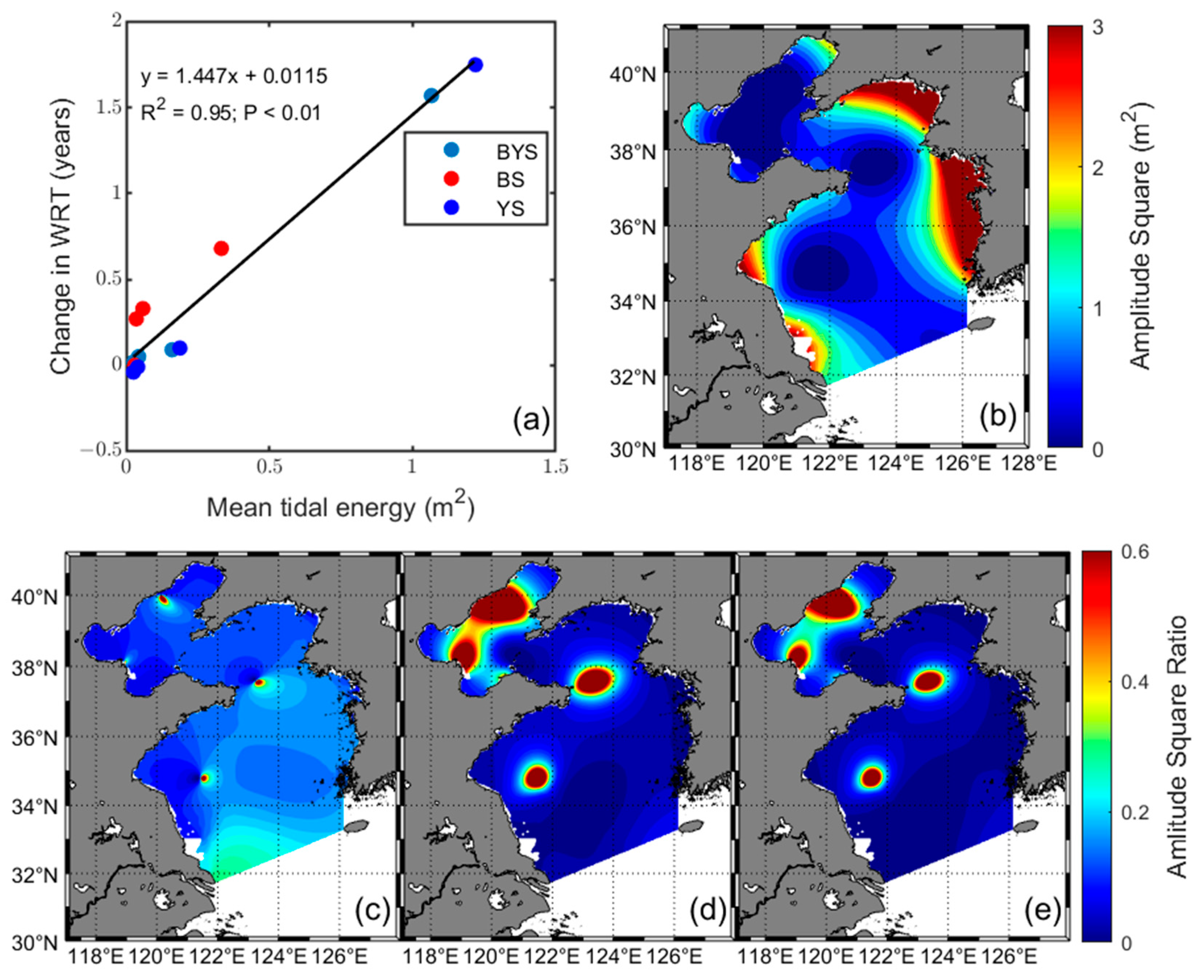
3.3. Effects of Tidal Constituents on the WRT
4. Discussion
4.1. Comparison with Previous Studies
4.2. Formation Mechanism of the Tidal-Driven WRT Pattern
4.3. Roles of Different Tidal Constituents on the WRT
5. Conclusions
Author Contributions
Funding
Data Availability Statement
Conflicts of Interest
Abbreviations
| WRT | water residence time |
| BYS | Bohai and Yellow Seas |
| LRC | Lagrangian residual currents |
| BS | Bohai Sea |
| YS | Yellow Sea |
References
- Bolin, B.; Rodhe, H. A note on the concepts of age distribution and transit time in natural reservoirs. Tellus 1973, 25, 58–62. [Google Scholar] [CrossRef]
- Delhez, É.J.; Heemink, A.W.; Deleersnijder, É. Residence time in a semi-enclosed domain from the solution of an adjoint problem. Estuar. Coast. Shelf Sci. 2004, 61, 691–702. [Google Scholar] [CrossRef]
- Takeoka, H. Fundamental concepts of exchange and transport time scales in a coastal sea. Cont. Shelf Res. 1984, 3, 311–326. [Google Scholar] [CrossRef]
- Messager, M.L.; Lehner, B.; Grill, G.; Nedeva, I.; Schmitt, O. Estimating the volume and age of water stored in global lakes using a geo-statistical approach. Nat. Commun. 2016, 7, 13603. [Google Scholar] [CrossRef]
- Lucas, L.V.; Deleersnijder, E. Timescale methods for simplifying, understanding and modeling biophysical and water quality processes in coastal aquatic ecosystems: A review. Water 2020, 12, 2717. [Google Scholar] [CrossRef]
- Gao, Y.; Jia, J.; Lu, Y.; Yang, T.; Lyu, S.; Shi, K.; Zhou, F.; Yu, G. Determining dominating control mechanisms of inland water carbon cycling processes and associated gross primary productivity on regional and global scales. Earth-Sci. Rev. 2021, 213, 103497. [Google Scholar] [CrossRef]
- Shen, J.; Du, J.; Lucas, L.V. Simple relationships between residence time and annual nutrient retention, export, and loading for estuaries. Limnol. Oceanogr. 2022, 67, 918–933. [Google Scholar] [CrossRef]
- John, S.; Muraleedharan, K.R.; Revichandran, C.; Azeez, S.A.; Seena, G.; Cazenave, P.W. What controls the flushing efficiency and particle transport pathways in a tropical estuary? Cochin Estuary, Southwest Coast of India. Water 2020, 12, 908. [Google Scholar] [CrossRef]
- Lin, L.; Liu, D.; Fu, Q.; Guo, X.; Liu, G.; Liu, H.; Wang, S. Seasonal variability of water residence time in the Subei Coastal Water, Yellow Sea: The joint role of tide and wind. Ocean Model. 2022, 180, 102137. [Google Scholar] [CrossRef]
- Jepsen, S.M.; Harmon, T.C.; Sadro, S.; Reid, B.; Chandra, S. Water residence time (age) and flow path exert synchronous effects on annual characteristics of dissolved organic carbon in terrestrial runoff. Sci. Total Environ. 2019, 656, 1223–1237. [Google Scholar] [CrossRef]
- Lin, L.; Fu, Q.; Jin, K.; Sun, Z. Investigation of water exposure time as a foundation for improving programs for coastal pollutant emission reduction. Ocean Coast. Manag. 2023, 245, 106880. [Google Scholar] [CrossRef]
- Du, J.; Shen, J. Water residence time in Chesapeake Bay for 1980–2012. J. Mar. Syst. 2016, 164, 101–111. [Google Scholar] [CrossRef]
- Xiong, J.; Shen, J.; Qin, Q. Exchange flow and material transport along the salinity gradient of a long estuary. J. Geophys. Res. Ocean. 2021, 126, e2021JC017185. [Google Scholar] [CrossRef]
- Xiong, J.; Shen, J.; Qin, Q.; Du, J. Water exchange and its relationships with external forcings and residence time in Chesapeake Bay. J. Mar. Syst. 2021, 215, 103497. [Google Scholar] [CrossRef]
- Luo, C.; Lin, L.; Shi, J.; Liu, Z.; Cai, Z.; Guo, X.; Gao, H. Seasonal variations in the water residence time in the Bohai Sea using 3D hydrodynamic model study and the adjoint method. Ocean Dyn. 2021, 71, 157–173. [Google Scholar] [CrossRef]
- Lin, L.; Liu, D.; Guo, X.; Luo, C.; Cheng, Y. Tidal effect on water export rate in the eastern shelf seas of China. J. Geophys. Res. Ocean. 2020, 125, e2019JC015863. [Google Scholar] [CrossRef]
- Stanev, E.V.; Ricker, M. Interactions between barotropic tides and mesoscale processes in deep ocean and shelf regions. Ocean Dyn. 2020, 70, 713–728. [Google Scholar] [CrossRef]
- Bao, R.; van der Voort, T.S.; Zhao, M.; Guo, X.; Montluçon, D.B.; McIntyre, C.; Eglinton, T.I. Influence of hydrodynamic processes on the fate of sedimentary organic matter on continental margins. Glob. Biogeochem. Cycles 2018, 32, 1420–1432. [Google Scholar] [CrossRef]
- Pei, Q.; Sheng, J.; Ohashi, K. Numerical Study of Effects of Winds and Tides on Monthly-Mean Circulation and Hydrography over the Southwestern Scotian Shelf. J. Mar. Sci. Eng. 2022, 10, 1706. [Google Scholar] [CrossRef]
- Safak, I.; Wiberg, P.L.; Richardson, D.L.; Kurum, M.O. Controls on residence time and exchange in a system of shallow coastal bays. Cont. Shelf Res. 2015, 97, 7–20. [Google Scholar] [CrossRef]
- Lin, S.; Sheng, J. Interactions between Surface Waves, Tides, and Storm-Induced Currents over Shelf Waters of the Northwest Atlantic. J. Mar. Sci. Eng. 2023, 11, 555. [Google Scholar] [CrossRef]
- Du, J.; Shen, J.; Zhang, Y.J.; Ye, F.; Liu, Z.; Wang, Z.; Wang, Y.; Yu, X.; Sisson, M.; Wang, H.V. Tidal response to sea-level rise in different types of estuaries: The Importance of Length, Bathymetry, and Geometry. Geophys. Res. Lett. 2018, 45, 227–235. [Google Scholar] [CrossRef]
- Wu, Z.; Zhou, C.; Wang, P.; Fei, Z. Responses of tidal dynamic and water exchange capacity to coastline change in the Bohai Sea, China. Front. Mar. Sci. 2023, 10, 1118795. [Google Scholar] [CrossRef]
- Guo, X.; Yanagi, T. Three-dimensional structure of tidal current in the East China Sea and the Yellow Sea. J. Oceanogr. 1998, 54, 651–668. [Google Scholar] [CrossRef]
- Liu, Z.; Lin, L.; Xie, L.; Gao, H. Partially implicit finite difference scheme for calculating dynamic pressure in a terrain-following coordinate non-hydrostatic ocean model. Ocean Model. 2016, 106, 44–57. [Google Scholar] [CrossRef]
- Mellor, G.L.; Yamada, T. Development of a turbulence closure model for geophysical fluid problems. Rev. Geophys. 1982, 20, 851–875. [Google Scholar] [CrossRef]
- Deleersnijder, E.; Campin, J.M.; Delhez, E.J. The concept of age in marine modelling: I. Theory and preliminary model results. J. Mar. Syst. 2001, 28, 229–267. [Google Scholar] [CrossRef]
- Delhez, É.J.; Deleersnijder, É. The concept of age in marine modelling: II. Concentration distribution function in the English Channel and the North Sea. J. Mar. Syst. 2002, 31, 279–297. [Google Scholar] [CrossRef]
- Lin, L.; Liu, Z. Partial residence times: Determining residence time composition in different subregions. Ocean Dyn. 2019, 69, 1023–1036. [Google Scholar] [CrossRef]
- Delhez, E.J.M. Transient residence and exposure times. Ocean Sci. 2006, 2, 1–9. [Google Scholar] [CrossRef]
- Delhez, É.J.; Deleersnijder, É. The boundary layer of the residence time field. Ocean Dyn. 2006, 56, 139–150. [Google Scholar] [CrossRef]
- Zimmerman, J.T.F. On the Euler-Lagrange transformation and the Stokes’ drift in the presence of oscillatory and residual currents. Deep. Sea Res. Part A Oceanogr. Res. Pap. 1979, 26, 505–520. [Google Scholar] [CrossRef]
- Shizuo, F.; Lian, J.; Wensheng, J. A Lagrangian mean theory on coastal sea circulation with inter-tidal transports I. Fundamentals. Acta Oceanol. Sin. 2008, 6, 1–16. [Google Scholar]
- Liu, G.; Liu, Z.; Gao, H.; Gao, Z.; Feng, S. Simulation of the Lagrangian tide-induced residual velocity in a tide-dominated coastal system: A case study of Jiaozhou Bay, China. Ocean Dyn. 2012, 62, 1443–1456. [Google Scholar] [CrossRef]
- Lin, L.; Liu, H.; Huang, X.; Fu, Q.; Guo, X. Effect of tides on river water behavior over the eastern shelf seas of China. Hydrol. Earth Syst. Sci. 2022, 26, 5207–5225. [Google Scholar] [CrossRef]
- Chen, D.X. Marine Atlas of Bohai Sea, Yellow Sea, East China Sea: Hydrology; China Ocean Press: Beijing, China, 1992. (In Chinese) [Google Scholar]
- Fang, G.; Wang, Y.; Wei, Z.; Choi, B.H.; Wang, X.; Wang, J. Empirical cotidal charts of the Bohai, Yellow, and East China Seas from 10 years of TOPEX/Poseidon altimetry. J. Geophys. Res. Oceans. 2004, 109, C11. [Google Scholar] [CrossRef]
- Xu, P.; Mao, X.; Jiang, W. Mapping tidal residual circulations in the outer Xiangshan Bay using a numerical model. J. Mar. Syst. 2016, 154, 181–191. [Google Scholar] [CrossRef]
- Wu, H.; Shen, J.; Zhu, J.; Zhang, J.; Li, L. Characteristics of the Changjiang plume and its extension along the Jiangsu Coast. Cont. Shelf Res. 2014, 76, 108–123. [Google Scholar] [CrossRef]
- Yao, Z.; He, R.; Bao, X.; Wu, D.; Song, J. M2 tidal dynamics in Bohai and Yellow Seas: A hybrid data assimilative modeling study. Ocean Dyn. 2012, 62, 753–769. [Google Scholar] [CrossRef]
- Hammons, T.J. Tidal power. Proc. IEEE 1993, 81, 419–433. [Google Scholar] [CrossRef]


| Region | Control Run | NoSemidiurnal | NoDiurnal | NoM2S2 | NoK1O1 | NoM2 | NoS2 | NoK1 | NoO1 |
|---|---|---|---|---|---|---|---|---|---|
| BYS (year) | 2.11 | 5.71 | 2.29 | 4.92 | 2.24 | 3.68 | 2.20 | 2.16 | 2.13 |
| BS (year) | 2.40 | 3.86 | 3.09 | 3.42 | 2.93 | 3.08 | 2.40 | 2.73 | 2.67 |
| YS (year) | 2.05 | 6.10 | 2.12 | 5.24 | 2.09 | 3.80 | 2.15 | 2.04 | 2.01 |
Disclaimer/Publisher’s Note: The statements, opinions and data contained in all publications are solely those of the individual author(s) and contributor(s) and not of MDPI and/or the editor(s). MDPI and/or the editor(s) disclaim responsibility for any injury to people or property resulting from any ideas, methods, instructions or products referred to in the content. |
© 2025 by the authors. Licensee MDPI, Basel, Switzerland. This article is an open access article distributed under the terms and conditions of the Creative Commons Attribution (CC BY) license (https://creativecommons.org/licenses/by/4.0/).
Share and Cite
Fu, Q.; Jiang, H.; Dong, C.; Jin, K.; Liu, X.; Lin, L. Tidal-Driven Water Residence Time in the Bohai and Yellow Seas: The Roles of Different Tidal Constituents. Water 2025, 17, 884. https://doi.org/10.3390/w17060884
Fu Q, Jiang H, Dong C, Jin K, Liu X, Lin L. Tidal-Driven Water Residence Time in the Bohai and Yellow Seas: The Roles of Different Tidal Constituents. Water. 2025; 17(6):884. https://doi.org/10.3390/w17060884
Chicago/Turabian StyleFu, Qingjun, Huichao Jiang, Chen Dong, Kangjie Jin, Xihan Liu, and Lei Lin. 2025. "Tidal-Driven Water Residence Time in the Bohai and Yellow Seas: The Roles of Different Tidal Constituents" Water 17, no. 6: 884. https://doi.org/10.3390/w17060884
APA StyleFu, Q., Jiang, H., Dong, C., Jin, K., Liu, X., & Lin, L. (2025). Tidal-Driven Water Residence Time in the Bohai and Yellow Seas: The Roles of Different Tidal Constituents. Water, 17(6), 884. https://doi.org/10.3390/w17060884