
Spatial Analysis to Retrieve SWAT Model Reservoir Parameters for Water Quality and Quantity Assessment


Abstract
1. Introduction
2. Data and Model
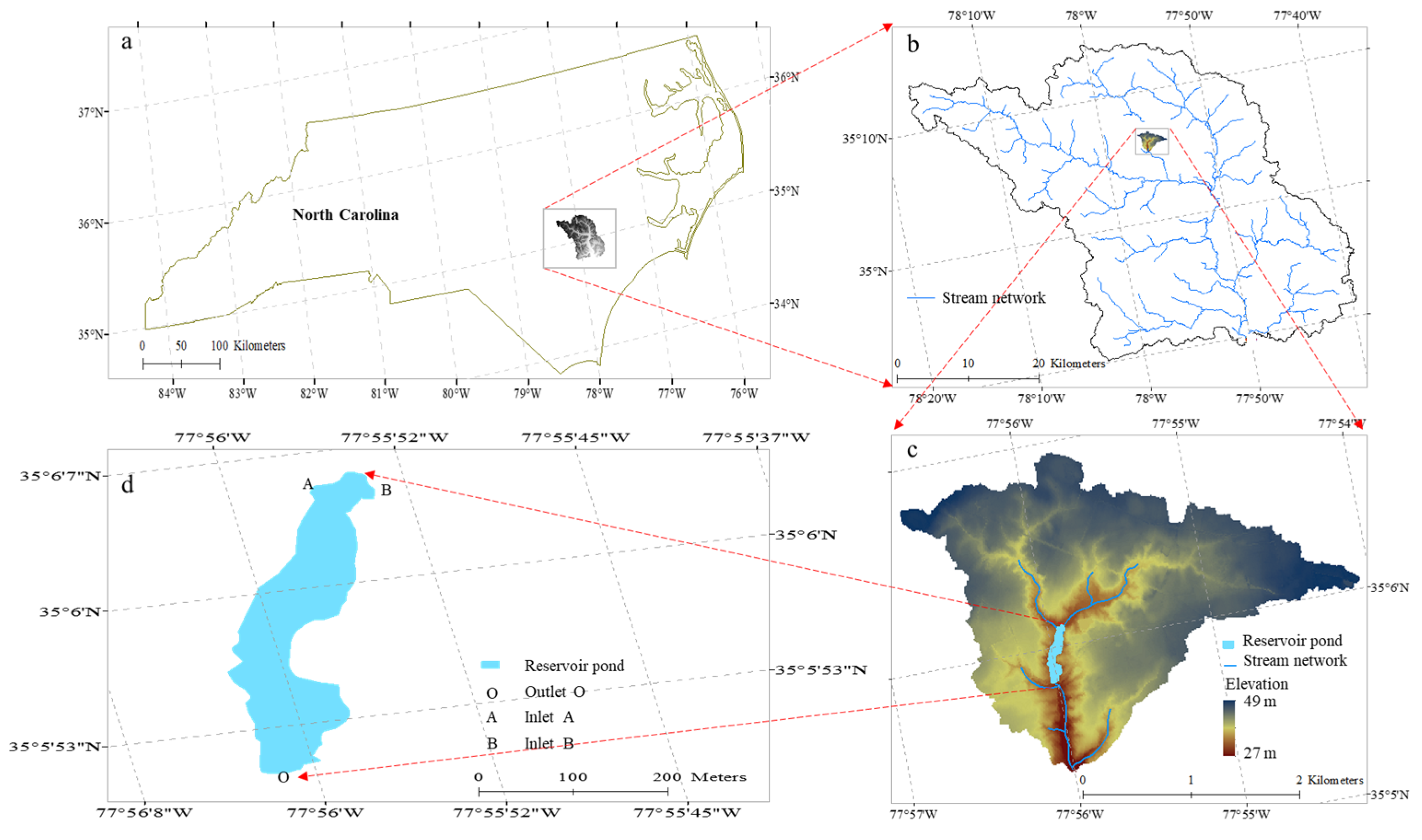
2.1. Data
2.2. SWAT Model
3. Spatial Analysis Procedure
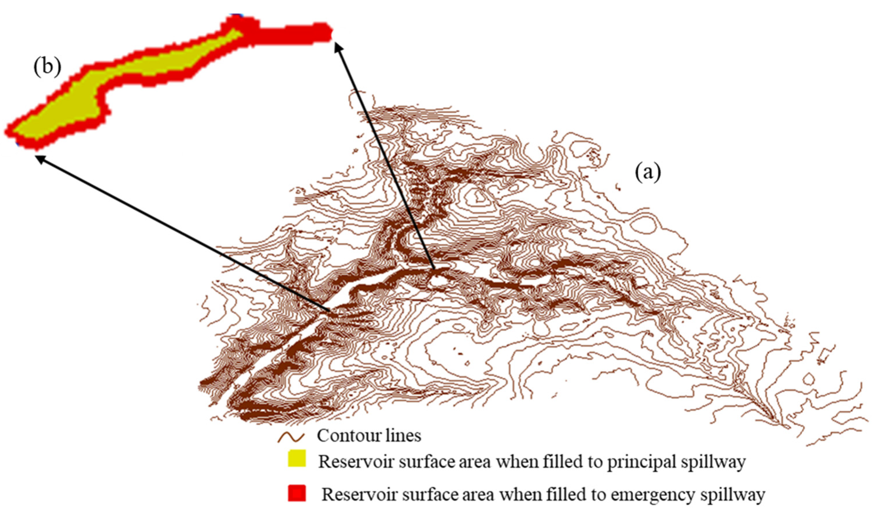
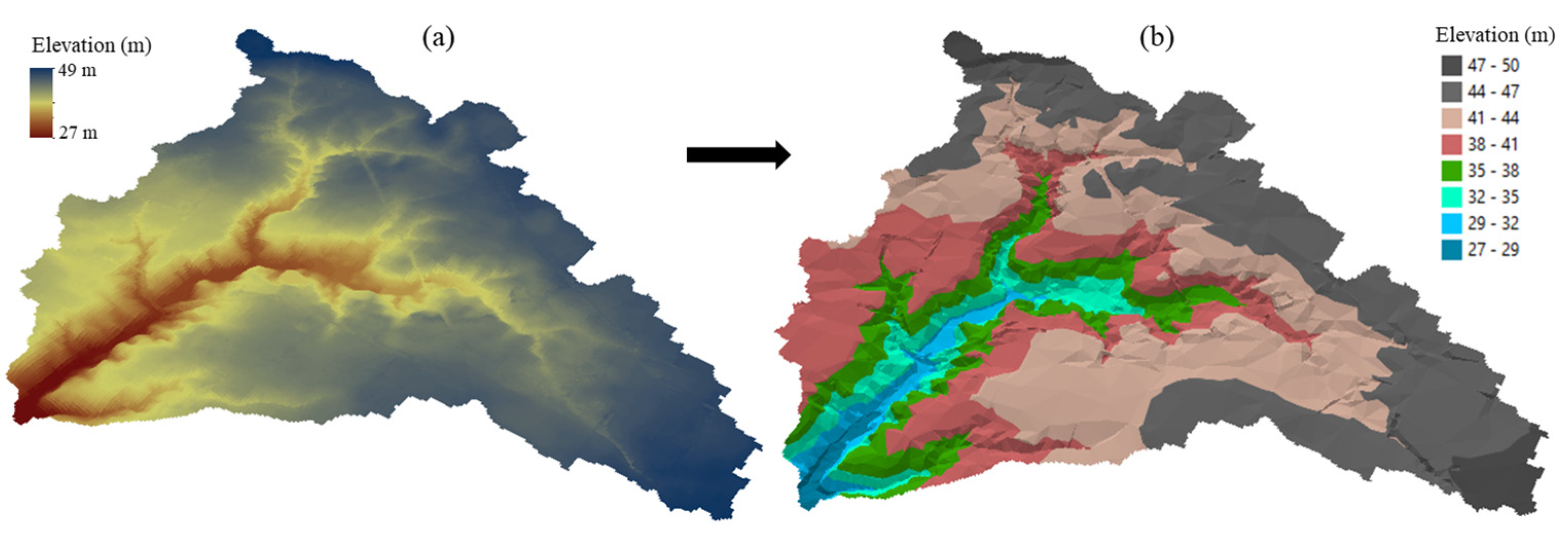
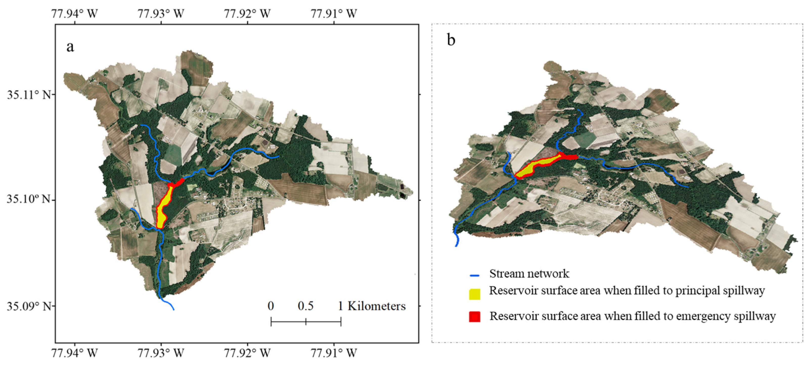
3.1. Step1: Estimating Reservoir Surface Area
3.2. Step 2: Estimating Reservoir Volume
4. Results and Discussion
5. Conclusions
Funding
Data Availability Statement
Conflicts of Interest
References
- Zhao, J.; Zhang, N.; Liu, Z.; Zhang, Q.; Shang, C. SWAT model applications: From hydrological processes to ecosystem services. Sci. Total Environ. 2024, 931, 172605. [Google Scholar] [CrossRef] [PubMed]
- White, M.J.; Arnold, J.G.; Bieger, K.; Allen, P.M.; Gao, J.; Čerkasova, N.; Gambone, M.; Park, S.; Bosch, D.D.; Yen, H.; et al. Development of a field scale SWAT+ Modeling Framework for the contiguous US. JAWRA J. Am. Water Resour. Assoc. 2022, 58, 1545–1560. [Google Scholar] [CrossRef]
- Sohoulande, D.C.D.; Szogi, A.A.; Novak, J.M.; Stone, K.C.; Martin, J.H.; Watts, D. Instream constructed wetland capacity at controlling phosphorus outflow under a long-term nutrient loading scenario: Approach using SWAT model. Model. Earth Syst. Environ. 2023, 9, 4349–4362. [Google Scholar] [CrossRef]
- Arnold, J.G.; Moriasi, D.N.; Gassman, P.W.; Abbaspour, K.C.; White, M.J.; Srinivasan, R.; Santhi, C.; Harmel, R.D.; Van Griensven, A.; Van Liew, M.W.; et al. SWAT: Model use, calibration, and validation. Trans. ASABE 2012, 55, 1491–1508. [Google Scholar] [CrossRef]
- Sohoulande, D.D.C. Assessment of sediment inflow to a reservoir using the SWAT model under undammed conditions: A case study for the Somerville reservoir, Texas, USA. Int. Soil Water Conserv. Res. 2018, 6, 222–229. [Google Scholar] [CrossRef]
- Wang, Z.; He, Y.; Li, W.; Chen, X.; Yang, P.; Bai, X. A generalized reservoir module for SWAT applications in watersheds regulated by reservoirs. J. Hydrol. 2023, 616, 128770. [Google Scholar] [CrossRef]
- Jordan, S.; Quinn, J.; Zaniolo, M.; Giuliani, M.; Castelletti, A. Advancing reservoir operations modelling in SWAT to reduce socio-ecological tradeoffs. Environ. Model. Softw. 2022, 157, 105527. [Google Scholar] [CrossRef]
- Kaur, A.; Paul, P.K.; Rudra, R.; Goel, P.K.; Daggupati, P. Evaluating and improving the simulation of channel and reservoir processes for streamflow and water quality modelling in the Lake Erie watersheds. Int. J. River Basin Manag. 2025, 1–16. [Google Scholar] [CrossRef]
- Liu, X.; Yang, M.; Meng, X.; Wen, F.; Sun, G. Assessing the impact of reservoir parameters on runoff in the Yalong River Basin using the SWAT Model. Water 2019, 11, 643. [Google Scholar] [CrossRef]
- Gao, H.; Birkett, C.; Lettenmaier, D.P. Global monitoring of large reservoir storage from satellite remote sensing. Water Resour. Res. 2012, 48. [Google Scholar] [CrossRef]
- Tsolakidis, I.; Vafiadis, M. Comparison of hydrographic survey and satellite bathymetry in monitoring Kerkini reservoir storage. Environ. Process. 2019, 6, 1031–1049. [Google Scholar] [CrossRef]
- Avisse, N.; Tilmant, A.; Müller, M.F.; Zhang, H. Monitoring small reservoirs' storage with satellite remote sensing in inaccessible areas. Hydrol. Earth Syst. Sci. 2017, 21, 6445–6459. [Google Scholar] [CrossRef]
- Sohoulande, C.D.; Szogi, A.A.; Novak, J.M.; Stone, K.C.; Martin, J.H.; Watts, D.W. Long-term nitrogen and phosphorus outflow from an instream constructed wetland under precipitation variability. Sustainability 2022, 14, 16500. [Google Scholar] [CrossRef]
- Homer, C.; Dewitz, J.; Yang, L.; Jin, S.; Danielson, P.; Xian, G.; Coulston, J.; Herold, N.; Wickham, J.; Megown, K. Completion of the 2011 national land cover database for the conterminous United States: Representing a decade of land cover change information. Photogramm. Eng. Remote Sens. 2015, 81, 345–354. [Google Scholar]
- Gan, T.Y.; Dlamini, E.M.; Biftu, G.F. Effects of model complexity and structure, data quality, and objective functions on hydrologic modeling. J. Hydrol. 1997, 192, 81–103. [Google Scholar] [CrossRef]
- Arnold, J.G.; Kiniry, J.R.; Srinivasan, R.; Williams, J.R.; Haney, E.B.; Neitsch, S.L. Soil and Water Assessment Tool Input/Output Documentation Version 2012; TR-439; Texas Water Resources Institute: College Station, TX, USA, 2013; 654p, Available online: https://hdl.handle.net/1969.1/149194 (accessed on 10 March 2025).
- Abbaspour, K.C. SWAT-CUP 2012 SWAT Calibration and Uncertainty Program—A User Manual. 2013. Available online: https://swat.tamu.edu/media/114860/usermanual_swatcup.pdf (accessed on 10 March 2025).
- Moriasi, D.N.; Gitau, M.W.; Pai, N.; Daggupati, P. Hydrologic and water quality models: Performance measures and evaluation criteria. Trans. ASABE 2015, 58, 1763–1785. [Google Scholar] [CrossRef]
- Willmott, C.J.; Ackleson, S.G.; Davis, R.E.; Feddema, J.J.; Klink, K.M.; Legates, D.R.; O’Donnell, J.; Rowe, C.M. Statistics for the evaluation and comparison of models. J. Geophys. Res. Ocean. 1985, 90, 8995–9005. [Google Scholar] [CrossRef]
- Yang, M.; Mou, Y.; Liu, S.; Meng, Y.; Liu, Z.; Li, P.; Xiang, W.; Zhou, X.; Peng, C. Detecting and mapping tree crowns based on convolutional neural network and Google Earth images. Int. J. Appl. Earth Obs. Geoinf. 2022, 108, 102764. [Google Scholar] [CrossRef]
- Huang, H.; Chen, Y.; Clinton, N.; Wang, J.; Wang, X.; Liu, C.; Gong, P.; Yang, J.; Bai, Y.; Zheng, Y.; et al. Mapping major land cover dynamics in Beijing using all Landsat images in Google Earth Engine. Remote Sens. Environ. 2017, 202, 166–176. [Google Scholar] [CrossRef]
- Hu, G.; Xiong, L.; Lu, S.; Chen, J.; Li, S.; Tang, G.; Strobl, J. Mathematical vector framework for gravity-specific land surface curvatures calculation from triangulated irregular networks. GIScience Remote Sens. 2022, 59, 590–608. [Google Scholar] [CrossRef]
- Marín-Comitre, U.; Gómez-Gutiérrez, Á.; Lavado-Contador, F.; Sánchez-Fernández, M.; Alfonso-Torreño, A. Using geomatic techniques to estimate volume–area relationships of watering ponds. ISPRS Int. J. Geo-Inf. 2021, 10, 502. [Google Scholar] [CrossRef]
- Novak, J.M.; Szogi, A.A.; Stone, K.C.; Chu, X.; Watts, D.W.; Johnson, M.H. Transport of Nitrate and Ammonium During Tropical Storm and Hurricane Induced Stream Flow Events from a Southeastern USA Coastal Plain In-Stream Wetland—1997 to 1999. In Advances in Hurricane Research-Modelling, Meteorology, Preparedness and Impacts; Hickey, K.R., Ed.; InTech: London, UK, 2012; pp. 139–158. [Google Scholar]
- Li, Y.; Gao, H.; Allen, G.H.; Zhang, Z. Constructing reservoir area–volume–elevation curve from TanDEM-X DEM data. IEEE J. Sel. Top. Appl. Earth Obs. Remote Sens. 2021, 14, 2249–2257. [Google Scholar] [CrossRef] [PubMed]
- Ouma, Y.O. Evaluation of multiresolution digital elevation model (DEM) from real-time kinematic GPS and ancillary data for reservoir storage capacity estimation. Hydrology 2016, 3, 16. [Google Scholar] [CrossRef]
- Nistoran, D.E.G.; Dragomirescu, A.; Ionescu, C.S.; Schiaua, M.; Vasiliu, N.; Georgescu, M. A procedure to develop elevation-area-capacity curves of reservoirs from depth sounding surveys. In Proceedings of the 2017 International Conference on ENERGY and ENVIRONMENT (CIEM), Bucharest, Romania, 19–20 October 2017; pp. 92–96. [Google Scholar] [CrossRef]
- Fassoni-Andrade, A.C.; De Paiva, R.C.D.; Fleischmann, A.S. Lake topography and active storage from satellite observations of flood frequency. Water Resour. Res. 2020, 56, e2019WR026362. [Google Scholar] [CrossRef]
- Sohoulande, D.D.C. Spectrum of climate change and streamflow alteration at a watershed scale. Environ. Earth Sci. 2017, 76, 653. [Google Scholar] [CrossRef]
- Meadows, M.; Jones, S.; Reinke, K. Vertical accuracy assessment of freely available global DEMs (FABDEM, Copernicus DEM, NASADEM, AW3D30 and SRTM) in flood-prone environments. Int. J. Digit. Earth 2024, 17, 2308734. [Google Scholar] [CrossRef]
- Moudrý, V.; Lecours, V.; Gdulová, K.; Gábor, L.; Moudrá, L.; Kropáček, J.; Wild, J. On the use of global DEMs in ecological modelling and the accuracy of new bare-earth DEMs. Ecol. Model. 2018, 383, 3–9. [Google Scholar] [CrossRef]


| Parameter | Description | Default Range | Range Values Used at Calibration and Validation |
|---|---|---|---|
| CN2 | Soil Conservation Service runoff curve number for moisture condition II | 35–98 | 25–92 |
| SOL_AWC | Soil available water capacity | 0–1 | 0.05–0.46 |
| SOL_K | Saturated hydraulic conductivity | 0–2000 | 51–1155 |
| Input Parameters for Reservoir (.res) | Definition/Description | Input Value |
|---|---|---|
| RES_ESA | surface area when filled to emergency spillway (ha) | 4.52 |
| RES_EVOL | volume when filled to emergency spillway (104 m3) | 2.54 |
| RES_PSA | surface area when filled to principal spillway (ha) | 3.04 |
| RES_PVOL | volume when filled to principal spillway (104 m3) | 0.6 |
| RES_VOL | Initial volume (104 m3) | 0.6 |
| RES_K | hydraulic conductivity (mm/hr) | 8 |
| IRESCO | Outflow simulation code (0 = uncontrolled reservoir) | 0 |
| RES_RR | Average daily principal spillway release rate (m3/s) | 0.06 |
| EVRSV | evaporation coefficient | 0.6 |
| WURESN | Average amount of water withdrawn each month for consumptive use (104 m3) | 0 |
Disclaimer/Publisher’s Note: The statements, opinions and data contained in all publications are solely those of the individual author(s) and contributor(s) and not of MDPI and/or the editor(s). MDPI and/or the editor(s) disclaim responsibility for any injury to people or property resulting from any ideas, methods, instructions or products referred to in the content. |
© 2025 by the author. Licensee MDPI, Basel, Switzerland. This article is an open access article distributed under the terms and conditions of the Creative Commons Attribution (CC BY) license (https://creativecommons.org/licenses/by/4.0/).
Share and Cite
Sohoulande, C.D.D. Spatial Analysis to Retrieve SWAT Model Reservoir Parameters for Water Quality and Quantity Assessment. Water 2025, 17, 834. https://doi.org/10.3390/w17060834
Sohoulande CDD. Spatial Analysis to Retrieve SWAT Model Reservoir Parameters for Water Quality and Quantity Assessment. Water. 2025; 17(6):834. https://doi.org/10.3390/w17060834
Chicago/Turabian StyleSohoulande, Clement D. D. 2025. "Spatial Analysis to Retrieve SWAT Model Reservoir Parameters for Water Quality and Quantity Assessment" Water 17, no. 6: 834. https://doi.org/10.3390/w17060834
APA StyleSohoulande, C. D. D. (2025). Spatial Analysis to Retrieve SWAT Model Reservoir Parameters for Water Quality and Quantity Assessment. Water, 17(6), 834. https://doi.org/10.3390/w17060834