A Bi-Level Optimization Framework for Water Supply Network Repairs Considering Traffic Impact

Abstract

Urban infrastructure systems, such as water supply and transportation networks, are highly interdependent, making them susceptible to cascading disruptions. This paper introduces a bi-level optimization framework designed to coordinate water supply network repairs while minimizing traffic impacts. The framework integrates a dynamic traffic assignment (DTA) model to evaluate the interplay between repair schedules and traffic conditions. The upper-level model generates and adjusts repair schedules, focusing on timing and location, while the lower-level model simulates the resulting traffic flow and travel time changes. Five optimization algorithms—adaptive differential evolution (ADE), genetic algorithm (GA), particle swarm optimization (PSO), simulated annealing (SA), and ant colony optimization (ACO)—are employed to identify repair plans that reduce traffic disruptions effectively. A case study in the Yangpu District of Shanghai demonstrates that the timing and spatial distribution of repairs significantly influence traffic flow. Among the tested algorithms, ADE achieves the lowest traffic impact, whereas SA excels in computational efficiency. The results highlight the importance of strategic scheduling in mitigating traffic disruptions by optimizing repair activities and leveraging traffic rerouting. This study provides a practical framework for urban planners to improve repair scheduling and minimize disruptions, contributing to more efficient infrastructure management. Future work could incorporate real-time data for adaptive scheduling and explore broader applications of the framework.

1. Introduction

Infrastructure networks, such as water supply and transportation systems, are essential to the functioning of modern society. As these networks grow increasingly interdependent, their vulnerabilities to disruptions rise, where a failure in one system can trigger cascading failures in others, causing widespread impacts. This concept of cascading failures, first examined by Buldyrev et al. [1] highlights the catastrophic consequences when interconnected systems fail to function cohesively. More recent studies have expanded on this work, exploring interdependencies in urban infrastructures and their broader implications for sustainability [2,3,4,5,6].

As urban infrastructure continues to age, the need for maintenance and repair intensifies, particularly in densely populated areas [7]. The challenge of maintaining water supply networks is compounded by the fact that such repairs often necessitate road closures, which disrupt transportation networks [5,8,9]. Jayasinghe et al. [10] highlighted the interdependencies between transport, water, and waste systems, stressing that repair schedules must be aligned to minimize the overall impact of maintenance work. For example, Kuliczkowska [5] demonstrated that the condition of underground sewer systems directly affects road safety, showing how closely these systems are linked. Moreover, numerous case studies illustrate the significant traffic impacts caused by water pipe repairs. Uddin [11] reviewed multiple instances in the US where water pipe failures led to road closures and even traffic accidents. Similarly, it was reported that nearly 4 million road openings occur annually in the UK for water pipe repairs, significantly disrupting traffic flow [12]. In China, a recent report noted 1723 pipeline failures in 2021, with 81.5% of them occurring in road areas [13], further illustrating the critical need for coordinated repair efforts. Understanding how to balance the need for timely infrastructure maintenance while minimizing disruptions to transportation has thus become a critical area of research.

Traditionally, repair scheduling has focused on optimizing a single network in isolation [14,15,16,17]. However, this approach frequently overlooks the broader effects of disruptions, particularly in complex urban environments where infrastructure systems are closely intertwined [10]. Imani and Hajializadeh [7] proposed a resilience assessment framework that emphasizes the importance of managing these interdependencies, especially during maintenance activities. Their research underscores the complexity of scheduling repairs in one system without causing undue disruptions in another.

Given the growing awareness of these challenges, research has increasingly focused on developing optimization algorithms to minimize disruptions across interdependent networks. Genetic algorithms (GA), for example, have been widely applied to optimize water distribution systems, as demonstrated by Prasad and Park [18], demonstrating their effectiveness in multi-objective optimization for water network design. More recent studies, such as those by Farmani and Butler [19], have integrated resilience into the optimization process, offering a more comprehensive approach to managing interdependent networks. In addition, adaptive differential evolution (ADE), particle swarm optimization (PSO), and ant colony optimization (ACO) have been employed to coordinate repair schedules across multiple systems. Another particular area of focus has been the use of dynamic traffic assignment (DTA) models, which capture real-time interactions between road closures and traffic conditions more accurately than traditional static traffic assignment methods. Marshall et al. [20] and Kachroo et al. [21] discuss the limitations of static models and advocated for DTA to better reflect the dynamic nature of traffic flow under varying conditions, such as those caused by repair work on water supply networks. This shift in modeling approaches is particularly relevant for urban environments, where traffic patterns are subject to rapid change.

Given these challenges, this paper introduces a bi-level optimization framework designed to coordinate water supply network repairs while maintaining the resilience of the transportation network. The upper-level model determines the repair schedule for the water supply network, focusing on when and where to conduct repairs. The lower-level model uses a DTA approach to simulate the resulting impact of road closures on the transportation network, assessing changes in travel speeds and total travel time. The model implementation was conducted using Python 3.8.8 and ArcGIS Pro 2.5.0 to process spatial data and analyze the impact of road closures. The goal is to minimize the disruptions to traffic while ensuring the efficient repair of the water supply system.

The novelty of this work lies in the integration of water supply network repair scheduling with dynamic traffic assignment to evaluate transportation network resilience. By considering the coupled nature of these networks, the proposed model provides a comprehensive tool for urban infrastructure management. The results can inform decision-makers about optimal repair strategies that minimize adverse impacts on both systems, contributing to more resilient urban infrastructures.

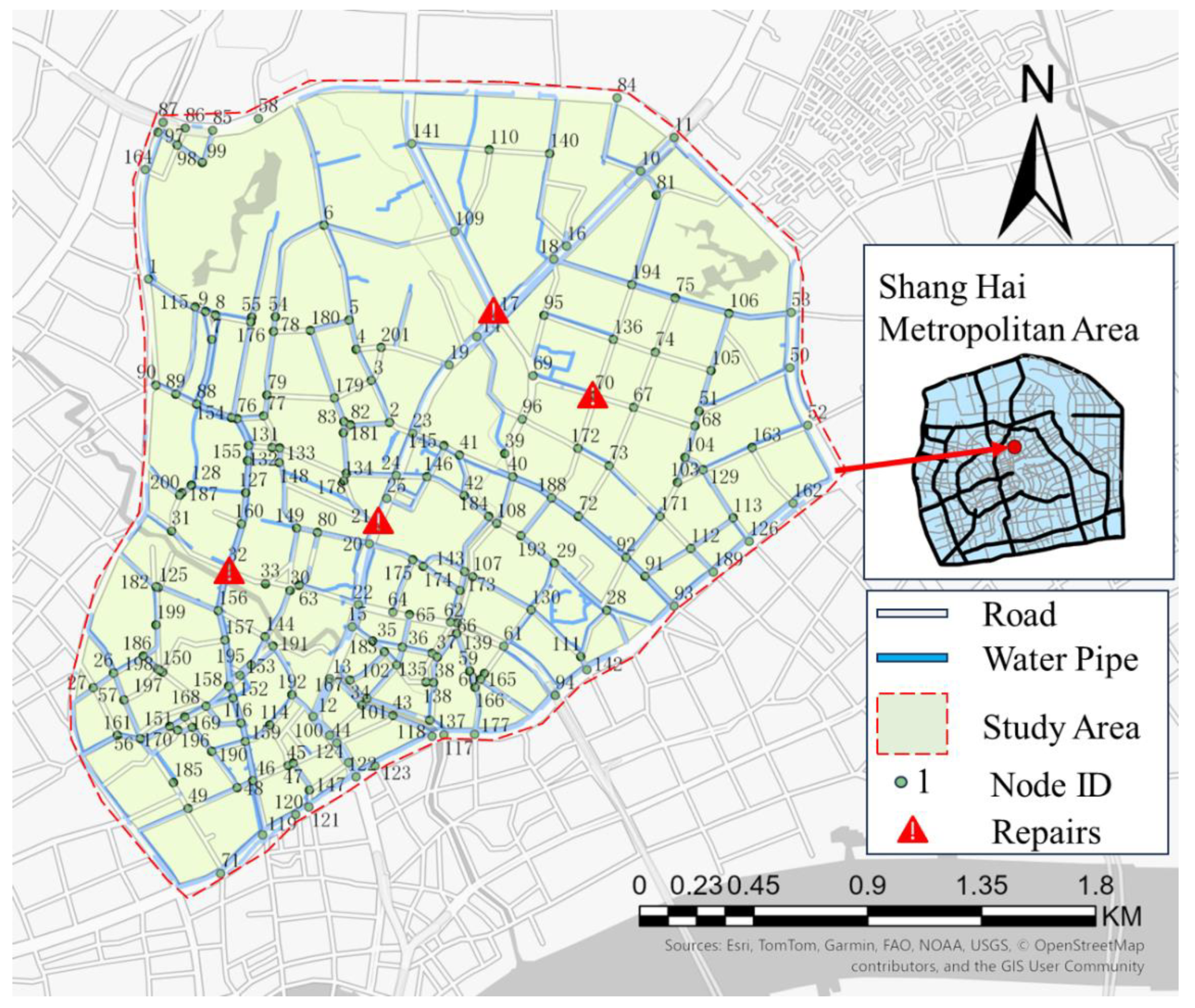
2. Study Area and Data

2.1. Study Area Description

The study area is located in central Yangpu District, Shanghai, China. It covers a total road length of 113.1 KM and a water supply network length of 60.3 KM, with a total area of 6.40 square kilometers. As shown in Figure 1, the major road nodes within this region are identified using Node IDs. This area is also notable for housing one of the oldest water supply networks in Shanghai, with the earliest pipelines dating back to 1926. While most of these oldest pipelines have been replaced over time, a significant portion of the network, particularly those installed in the 1950s, remains in use today. The presence of these aging pipelines adds to the complexity of managing both road and water infrastructure in this region.

Building on findings from relevant studies, it was observed that during the extreme cold wave period between 2020 and 2021 in Shanghai, numerous pipe segments experienced failures, including bursts and leaks, with an average of four incidents per day [22]. The cold wave events resulted in a sharp temperature drop, with minimum recorded air temperatures reaching −6.5 °C during the first cold wave and −7.5 °C during the second [22]. Although the pipelines are buried below the freezing depth, the prolonged duration of subzero temperatures (101 h and 125 h, respectively) and rapid temperature fluctuations (a drop of up to 23.5 °C within 48 h) significantly affected the pipe network [22]. The soil’s thermal lag and temperature blocking effect contributed to delayed cooling, but once the low temperature penetrated, it caused an increase in pipe stress and eventual failures. Consequently, this study adopts extreme cold waves as the research scenario. Based on safety evaluations conducted by the water supply company, four high-risk pipe segments were identified as being particularly vulnerable to failures during cold waves. This study assumes simultaneous failure events at these segments under such conditions and explores how to prioritize repair efforts by considering traffic impact factors.

The proposed repair locations, marked in Figure 1, are detailed in

Table 1. Repair locations in study area.

Node ID	Road Class	Pipe Type	Failure Type
17	Primary and Primary	DN 500, iron	Leak
21	Primary and Primary	DN 1200, iron	Leak
32	Primary and Primary	DN 300, cast iron	Leak
70	Secondary and Secondary	DN 300, cast iron	Leak

. Each location is identified by a “Node ID” and includes information on road class, pipe type, and failure type. The “Road Class” column indicates the classification of the two intersecting roads at each node, reflecting the importance and traffic volume of the roads involved. The “Pipe Type” column provides the pipe diameter (mm) and material, while the “Failure Type” column specifies the type of failure.

2.2. Data Sources

To effectively simulate the impact of water supply network repairs on the transportation system, a range of data inputs from both networks are integrated into the model. These inputs include detailed information on pipe characteristics, repair types, crew availability, road capacities, and traffic demand.

Table 2. Dataset of the study area.

Type	Data Source	Description	Usage in Simulation
Water Supply Network	Pipe GIS data	Includes spatial and attribute information of pipes, such as diameters, materials, etc.	Used to calculate repair times, influencing the duration and crew allocation based on the Hazus Earthquake Model Technical Manual
	Repair Types	Types of repairs, such as leaks and burst pipes	Determines the repair time calculation based on the type of repair (leak or burst)
	Repair Crew Data	Information on available crew size	Used to dynamically allocate crew resources based on the impact of repairs on the transportation network
	Repair Time Formula	Hazus Earthquake Model Technical Manual	Provides the formula to calculate the repair duration based on pipe diameter and repair type
Transportation Network	Road GIS Data	Contains spatial and attribute information of road segments, including road hierarchy and width	Used to model network topology and road capacity
	Road Capacity Data	Capacity of roads in the transportation network	Road capacities are adjusted dynamically based on the proximity and severity of the repair activities
	Traffic Demand Data	OD (Origin–Destination) matrices	Reflects traffic demand and volume for different times of day, influencing dynamic traffic assignment

summarizes the key data sources and their roles in the simulation process. The water supply network data include GIS-based pipe information, repair types, and crew resources, which are used to calculate repair times and dynamically allocate crews. For the transportation network, road capacity data and traffic demand matrices are essential for modeling dynamic traffic assignment during repair scenarios.

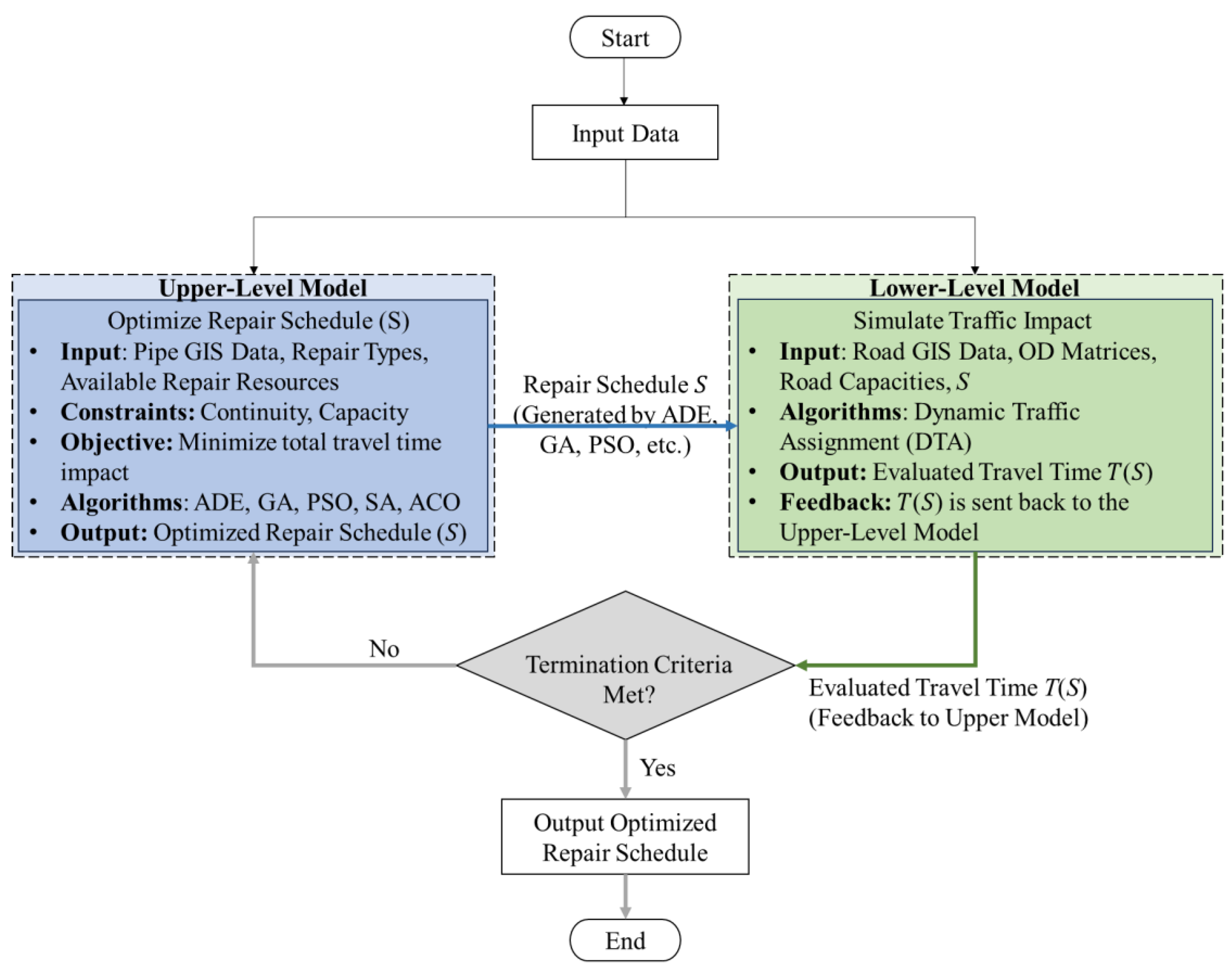
3. Methodology

In this study, a bi-level optimization model is developed to coordinate water supply network repairs with transportation network resilience. The model comprises two interconnected levels: the upper-level model and the lower-level model.

As illustrated in Figure 2, the upper-level model generates and iteratively refines the repair schedule S, including decisions on repair locations and timing. This repair schedule is then passed to the lower-level model, which evaluates its impact on traffic using a Dynamic Traffic Assignment (DTA) framework. Feedback from the lower-level model—quantified in terms of total travel time or traffic disruptions—is subsequently used by the upper-level model to adjust the repair schedule. This iterative process continues until predefined termination criteria are met, such as convergence of the objective function or reaching the maximum number of iterations.

The flowchart in Figure 2 visually represents this iterative process. The key components include the following points.

• Input Data: Pipe GIS data, repair types, crew availability, and traffic origin-destination (OD) matrices.
• Upper-Level Model: Employs optimization algorithms, such as adaptive differential evolution (ADE), genetic algorithm (GA), and particle swarm optimization (PSO) to minimize traffic disruptions by optimizing repair schedules.
• Lower-Level Model: Simulates the dynamic traffic response to road closures caused by repairs using the DTA approach.
• Feedback Loop: The repair schedule is iteratively updated based on traffic simulation results, ensuring a balance between repair efficiency and minimizing traffic disruptions.
• Termination Criteria Check: The optimization process continues until predefined termination criteria are met. These criteria include (1) convergence of the objective function, where improvements in total travel time impact become negligible over consecutive iterations; (2) reaching the maximum number of iterations or generations; (3) for the simulated annealing (SA) algorithm, the termination condition is met when the temperature falls below 0.001, following an exponential cooling schedule; and (4) for certain algorithms like ADE, ACO, and GA, an early stopping mechanism is applied, terminating the optimization if no improvement is observed over 10 consecutive iterations. These stopping conditions ensure computational efficiency while maintaining solution quality.

This bi-level optimization framework provides a practical tool for managing interdependent infrastructure systems, integrating repair scheduling with traffic resilience considerations to achieve the dual objectives of efficient repair execution and reduced traffic disruptions.

3.1. Upper-Level Model: Water Supply Network Repair Scheduling

The upper-level model is responsible for determining the optimal scheduling of water supply network repairs while minimizing the impact on traffic. It decides when and where each repair task should occur, ensuring that disruptions are minimized and the repair efficiency is maximized. The input data for the upper-level model consists of pipe GIS data (diameter, material, and spatial attributes), repair types (leak or burst), repair crew availability, and the repair time calculation formula, as summarized in Table 2. Additionally, traffic demand data (origin–destination matrices) are incorporated to assess the impact of road closures. These inputs are critical for determining the repair schedule while minimizing transportation disruptions.

3.1.1. Decision Variables

• S (Repair Schedule Set): The set of repair schedules, where each $s_i$ represents the start time and duration of repair task i. It is defined as

$$S=\{s_i=(t_{start}^i,d_i)\mid i\in N\},$$

(1)

where

$t_{start}^i$ is the start time of repair task i;

$d_i$ is its duration;

N is the set of all repair tasks.

• x_i,t (Repair Activation Indicator): A binary decision variable, where

$$x_{i,t}=\{\begin{array}{cccc}1,& \mathrm{if}\mathrm{repair}\mathrm{task}i\mathrm{is}\mathrm{active}\mathrm{at}\mathrm{time}t& & \\ 0,& \mathrm{o}\mathrm{t}\mathrm{h}\mathrm{e}\mathrm{r}\mathrm{w}\mathrm{i}\mathrm{s}\mathrm{e}& & \end{array}.$$

(2)

This variable ensures that each repair task is either in progress or inactive at a given time.

• C (Repair Crew Capacity): The maximum number of repair crews available at any given time.

3.1.2. Objective Function

The objective function of the upper-level model is to minimize the total traffic impact caused by repair activities, defined as the difference between the total travel time under a repair schedule T(S) and the baseline travel time $T_{\mathrm{b}\mathrm{a}\mathrm{s}\mathrm{e}}$:

$$\underset{S}{\mathrm{m}\mathrm{i}\mathrm{n}}Z(S)=T(S)-T_{\mathrm{b}\mathrm{a}\mathrm{s}\mathrm{e}},$$

(3)

where

$Z(S)$ is the total travel time impact caused by the repair schedule;

$T_{\mathrm{b}\mathrm{a}\mathrm{s}\mathrm{e}}$ is the baseline total travel time calculated by simulating the transportation network without any repair activities, serving as a fixed reference for comparing different repair scenarios;

T(S) is calculated by summing the product of traffic volume V_r(t) and travel time T_r(t) across all road segments and time periods (Equation (13)).

3.1.3. Constraints

The repair scheduling process is subject to the following constraints.

• Repair Duration Constraint: Each repair task must be completed within a continuous time window.

$$t_i+d_i\le T,\forall i\in S,$$

(4)

where

$t_i$ is the start time of repair i;

$d_i$ is the duration of repair i;

$T$ is the total available time horizon for repairs.

• Crew Allocation Constraint: The total number of repair crews assigned at any given time should not exceed the available limit.

$$\sum _{i\in S}{x}_{i,t}\le C,\forall t\in T,$$

(5)

where C is the maximum number of repair crews available at any time.

In addition, crew resources are dynamically allocated based on the traffic impact of each repair task. Tasks that cause greater disruptions are prioritized with more crew resources to minimize their duration and mitigate their impact on the transportation network.

• Simultaneous Repairs Constraint: To ensure efficient use of resources and minimize disruptions, we impose a simultaneous repairs constraint, meaning no more than two repair tasks occur at the same time. This constraint accounts for local workforce limitations, the availability and spatial constraints of heavy machinery (e.g., excavators, welding equipment), and the need to control road occupancy and traffic disruptions.

$$\begin{array}{c}\sum _{i\in S}{x}_{i,t}\le 2,\forall t\in T.\end{array}$$

(6)

By enforcing these constraints, the upper-level model ensures that repairs are scheduled efficiently, balancing infrastructure maintenance needs with traffic impact considerations.

3.1.4. Computation Process

The upper-level model follows an iterative optimization process to determine the optimal repair schedule while minimizing traffic disruptions. The computation process consists of the following steps.

• Step 1: Initialize the Repair Schedule

An initial set of repair schedules is generated, either randomly or based on heuristic rules. Each schedule specifies the repair locations and start times while ensuring that constraints on repair continuity and resource availability are met.

• Step 2: Evaluate Traffic Impact Using the Lower-Level Model

The generated repair schedule is passed to the lower-level DTA model, which simulates traffic flow and calculates the resulting total travel time impact. This step quantifies the effect of the repair activities on the transportation network.

• Step 3: Optimization Algorithm Iteration

Based on the travel time feedback from the lower-level model, the upper-level optimization algorithm modifies the repair schedule. The optimization process ensures that

• The number of simultaneous repairs does not exceed the allowed limit;
• Repair continuity is maintained over time;
• Crew resource constraints are satisfied.

• Step 4: Update the Repair Schedule

The newly generated schedules from the optimization process replace previous solutions, provided they result in a lower total travel time impact.

• Step 5: Check Termination Criteria

The iterative optimization process continues until one of the following stopping conditions is met.

• Convergence: The improvement in total travel time impact becomes negligible over consecutive iterations.
• Maximum iterations reached: The predefined maximum number of iterations is exhausted.
• Patience parameter: For certain algorithms, if no improvement is observed over a set number of iterations, the process is terminated early.

• Step 6: Output the Optimal Repair Plan

Once the optimization process converges, the final repair schedule is selected as the solution that minimizes the overall traffic impact while ensuring all repair tasks are completed within the given constraints.

3.2. Lower-Level Model: Dynamic Traffic Assignment (DTA)

The lower-level model evaluates the traffic impact of a given repair schedule by simulating vehicle flows on the affected road network through a DTA [23] approach. It dynamically assigns traffic based on congestion patterns and road capacity reductions due to ongoing repairs. The input data for the lower-level model include road network topology, road capacity data, and traffic demand data. The road network topology defines the structure of the transportation network, including connectivity between nodes and segment characteristics. The road capacity data, obtained from GIS-based road inventory datasets, determine the maximum allowable vehicle flow on each segment. The traffic demand data reflect vehicle movement patterns throughout different time periods. The DTA model dynamically updates these inputs to simulate the impact of repair-induced road capacity reductions, adjusting traffic flow accordingly.

3.2.1. Key Variables

• V_r(t) (Traffic Volume on Road Segment r): The number of vehicles traveling on road segment r at time t, which dynamically changes based on road capacity constraints and repair activities.
• Q_r(t) (Time-Dependent Traffic Demand on Road Segment r): The number of vehicles that intend to travel on road segment r at time t, derived from origin–destination (OD) data.
• T_r(t) (Travel Time on Road Segment r): The estimated travel time for vehicles on road r at time t, calculated using the BPR function (Equation (11)).
• $C_r\left(S_t\right)$ (Remaining Road Capacity): The available capacity of road segment r at time t, affected by the repair schedule S. It is computed as

$$C_r(S_t)=C_r^0-\sum _{i\in N}{x}_{i,t}\cdot {\delta }_{i,r,}$$

(7)

where

$C_r^0$ is the original capacity of road r before any repair activities;

${\delta }_{i,r}$ is an indicator variable, where ${\delta }_{i,r}$ = 1 if repair task i affects road r, and 0 otherwise.

3.2.2. Constraints

• Traffic Flow Conservation: Ensures that the total incoming traffic at a road segment equals the total outgoing traffic, preserving flow continuity.

$$\begin{array}{c}\sum _{o\in O}{d}_{or}(t)=\sum _{d\in D}{V}_{rd}(t),\forall r\in R,t\in T\end{array},$$

(8)

where $d_{or}(t)$ represents traffic demand from origin o to road segment r, and $V_{rd}(t)$ represents traffic flow from r to destination d.

• Capacity Constraint: Restricts the traffic volume on each road segment to not exceed its available capacity at a given time, accounting for reduced capacity due to repairs.

$$V_r(t)\le C_r(t),\forall r\in R,t\in T,$$

(9)

where $C_r\left(t\right)$ is the dynamically updated road capacity based on repair activities.

• Travel Time Function: The travel time function follows the Bureau of Public Roads (BPR) function [24], which models how congestion impacts travel time based on traffic volume and road capacity.

$$T_r(t)=T_r^0(1+\alpha {({\displaystyle \frac{V_r(t)}{C_r(t)}})}^{\beta }),$$

(10)

where

$T_r^0$ is the free-flow travel time on road r;

α and β are parameters that describe the sensitivity of travel time to congestion.

By incorporating these constraints, the lower-level model ensures that the impact of road capacity reductions due to repairs is properly reflected in traffic simulations, enabling better coordination of repair activities to minimize disruptions.

3.2.3. Computation Process

The lower-level model evaluates the traffic impact of a given repair schedule S by simulating network-wide traffic flow dynamics. The computation process consists of the following four main steps.

• Step 1: Modify Road Network Conditions Based on Repair Schedule S

The repair schedule S determines the affected road segments and the extent of their capacity reduction. The remaining road capacity for a segment r at time t is computed as

$$C_r(t)=C_r^{\mathrm{o}\mathrm{r}\mathrm{i}\mathrm{g}}\cdot {\alpha }_r(t),$$

(11)

where

$C_r^{\mathrm{o}\mathrm{r}\mathrm{i}\mathrm{g}}$ is the original capacity of road segment r;

${\alpha }_r(t)$ is the capacity reduction factor, which depends on the repair activity at segment ${\alpha }_r(t)$ = 1, where there is no reduction, and ${\alpha }_r(t)$ < 1, which indicates partial capacity loss.

• Step 2: Perform Dynamic Traffic Assignment (DTA)

Once road capacities are adjusted, traffic is dynamically reassigned based on updated congestion conditions. The traffic volume on road segment r at time t, denoted as V_r(t), is determined as

$$V_r(t)=\sum _{r\in R}{Q}_r(t)\cdot {\delta }_r(t),$$

(12)

where

R is the set of all road segments;

$Q_r(t)$ is the total traffic demand passing through road segment r at time t, aggregated from OD pairs;

${\delta }_r(t)$ is a binary indicator function, equal to 1 if road r is part of the shortest path for a given OD pair at time t, and 0 otherwise.

• Step 3: Compute System-Wide Travel Time T(S)

The total travel time T(S) is computed as the sum of travel times across all road segments, weighted by the traffic volume:

$$T(S)={\sum }_{r\in R}{\int }_0^T{V}_r(t)\cdot T_r(t)dt,$$

(13)

where

$T_r(t)$ is the travel time on road segment r at time t;

$V_r(t)$ is the number of vehicles traveling on road segment r at time t;

• Step 4: Provide Feedback to the Upper-Level Model

The computed travel time T(S) is sent as feedback to the upper-level model, which uses it to calculate Z(S) to iteratively refine the repair schedule S. The optimization process continues until a termination condition is met, such as convergence of T(S) or reaching a predefined iteration limit.

3.3. Repair Scheduling Strategy

3.3.1. Water Supply Network

• Repair Time

Repair durations are computed based on the type of repair (leak or burst) and the diameter of the pipes, utilizing a predefined repair time function. As shown in

Table 3. Restoration functions for water supply networks.

Class	Diameter from: [mm]	Diameter to: [mm]	# (Number of) Fixed Breaks/Day/Worker	# Fixed Leaks/Day/Worker	# Available Workers for Leaks and Breaks	Priority
a	1500	7600	0.2	0.4	100	1 (Highest)
b	900	1500	0.2	0.4	100	2
c	500	900	0.2	0.4	100	3
d	300	500	0.5	1	100	4
e	200	300	0.5	1	100	5
u	<200, or Unknown Diameter		0.5	1	100	6 (Lowest)

, this function is derived from the Hazus Earthquake Model Technical Manual [25], published by the American Federal Emergency Management Agency (FEMA), accounting for crew size, repair type, and the pipe’s specifications.

In real-world water supply network maintenance, repair teams typically consist of multiple specialized roles, including pipefitters, welders, electricians, mechanics, inspectors, and safety coordinators. The distribution of these roles varies based on network complexity and operational requirements. Generally, pipefitters (40–50%) form the largest proportion, responsible for pipe installation, replacement, and leak repairs. Welders (5–10%) handle metal pipe welding and crack repairs, while electricians (10–15%) manage pump stations, control systems, and remote monitoring equipment. Mechanics (10–15%) maintain mechanical components, such as valves and pressure regulators, and inspectors (5–10%) conduct non-destructive testing using advanced tools like CCTV cameras and pressure sensors. Safety personnel ensure compliance with operational safety standards.

Given the complexity of urban infrastructure, multi-role assignments are common. For instance, in smaller teams or emergency response situations, pipefitters may also perform welding, electricians may handle automation control, and inspectors may assist in minor repairs. For simplicity in model computation, we assume a total repair crew size of 40 without explicitly specifying the number of workers assigned to each role.

• Dynamic Crew Allocation

The total available number of repair crews is set at 40, based on data provided by the managing authority and actual operational conditions. The allocation of crews to each repair location is dynamically adjusted according to the expected impact on the transportation network. Locations that are expected to cause greater traffic disruptions will receive more crew resources to minimize the duration of repairs and, consequently, reduce their impact on traffic. The dynamic crew allocation strategy ensures that the available resources are utilized efficiently by prioritizing high-impact locations, allowing for more crews to be allocated where they are most needed while maintaining the overall crew capacity limit of 40.

3.3.2. Transportation Network

• Road Capacity

The capacity of each road is directly impacted by water supply network repairs. Roads affected by repair activities see their capacity reduced in proportion to the severity of the disruption. This capacity reduction is dynamically adjusted based on the repair location and duration. For pipelines with a diameter of DN500 or greater, repair activities typically occupy a larger portion of the roadway, thus reducing the road capacity to 20% of its original capacity. For pipelines with a diameter below DN500, repair work generally occupies only half of the road, resulting in a road capacity of 40% of its original capacity.

• Traffic Demand

The traffic demand data are derived from the origin–destination (OD) data. These demand data are time-sensitive, reflecting peak and off-peak traffic periods.

3.3.3. Time Points

The simulation is conducted at 8 distinct time points, spanning from 9:00 AM to 4:00 PM, with a 60 min interval between each time slot. The repair schedule is allowed to vary across these time points, and the impact on the transportation network is evaluated separately for each period.

By integrating these parameters into the simulation, we can effectively assess the trade-offs between minimizing the disruption to traffic flow and completing essential water supply network repairs.

4. Optimization Approach

In this study, we employ five optimization algorithms—adaptive differential evolution (ADE), genetic algorithm (GA), particle swarm optimization (PSO), simulated annealing (SA), and ant colony optimization (ACO)—to optimize the water supply network repair schedule, aiming to minimize the disruption to the transportation network.

Although metaheuristic optimization approaches are more commonly applied to transportation and network optimization problems, they offer several advantages for water network repair scheduling. Given the complex interplay between repair schedules and dynamic traffic conditions, these algorithms provide robust solutions for multi-objective optimization under uncertainty. Their adaptability in handling large-scale infrastructure problems makes them particularly suitable for optimizing repair schedules while minimizing disruptions. This study demonstrates how these methods can be effectively integrated into water network restoration, expanding their applicability in urban infrastructure management. While each algorithm operates with different mechanisms, they share a common optimization framework.

4.1. Algorithmic Framework for Optimization

The optimization process in this study follows a common structure across all algorithms:

(a)

Population Initialization: A population of candidate solutions (repair schedules) is initialized, where each individual represents a possible solution for the water supply network repairs. Each individual is encoded as a vector S, where the elements of S correspond to repair locations and times.

(b)

Fitness Evaluation: For each individual, the fitness is evaluated based on the total travel time T(S), calculated using the DTA model. The objective is to minimize this travel time across the population.

(c)

Selection: Individuals are selected for the next generation based on their fitness. The selection mechanism varies between algorithms but generally favors individuals with lower travel times.

(d)

Termination: The optimization process continues until a stopping criterion is met, such as reaching the maximum number of generations or achieving convergence.

The common structure described above provides a foundation for understanding the role of optimization algorithms in addressing the repair scheduling problem. Building on this foundation, the following sections explore the specific algorithms implemented in this study, analyzing their operational principles, parameter tuning strategies, and comparative performance.

4.2. Adaptive Differential Evolution (ADE)

ADE is an advanced variant of the differential evolution (DE) algorithm, designed to improve convergence speed and solution quality in continuous optimization problems [26]. It is a population-based algorithm that adapts key parameters dynamically during the optimization process. It is well-suited for continuous optimization in non-linear search spaces.

• Mutation and Crossover

In ADE, the mutation factor F and crossover probability CR are adapted at each generation to balance exploration and exploitation of the search space. The mutation vector $V_i$ for each individual i is generated by

$$V_i=X_{r_1}+F\cdot (X_{r_2}-X_{r_3}),$$

(14)

where $X_{r_1},X_{r_2},X_{r_3}$ are randomly selected individuals from the population, and F is the adaptive mutation factor. The trial vector $U_i$ is created by combining $V_i$ with the current solution $X_i$, controlled by the crossover probability CR.

• Adaptive Parameters

The mutation factor F and crossover probability CR are updated as follows:

$$F_i=F_{min}+\mathrm{r}\mathrm{a}\mathrm{n}\mathrm{d}\left(\mathrm{0,1}\right)\cdot \left(F_{max}-F_{min}\right)$$

(15)

$$C{R}_i=C{R}_{min}+\mathrm{r}\mathrm{a}\mathrm{n}\mathrm{d}(\mathrm{0,1})\cdot (C{R}_{max}-C{R}_{min}).$$

(16)

These adaptive strategies allow ADE to explore the solution space efficiently early in the process and refine solutions later.

4.3. Genetic Algorithm (GA)

The GA is an evolutionary algorithm inspired by natural selection. In GA, a population of solutions evolves over successive generations to find an optimal or near-optimal solution [27].

• Crossover and Mutation

In GA, crossover and mutation are the key operators for generating new solutions. The crossover operator combines two parent solutions by swapping portions of their repair schedules, producing two offsprings. For single-point crossover,

$${\mathrm{c}\mathrm{h}\mathrm{i}\mathrm{l}\mathrm{d}}_1=[{\mathrm{p}\mathrm{a}\mathrm{r}\mathrm{e}\mathrm{n}\mathrm{t}}_1(1:k),{\mathrm{p}\mathrm{a}\mathrm{r}\mathrm{e}\mathrm{n}\mathrm{t}}_2(k+1:m)],$$

(17)

where k is a randomly chosen crossover point. Mutation is applied by flipping the values of some bits in the binary-encoded repair schedules, ensuring diversity in the population.

• Selection

GA uses roulette wheel selection, where individuals with higher fitness are more likely to be chosen for reproduction. The selection probability $P(x_i)$ for each individual $x_i$ is proportional to its fitness:

$$P(x_i)={\displaystyle \frac{F(x_i)}{\sum _{j=1}^p\hspace{1em}F(x_j)}},$$

(18)

where $F(x_i)$ is the fitness of individual $x_i$, and p is the population size.

4.4. Particle Swarm Optimization (PSO)

PSO is a population-based algorithm inspired by the social behavior of birds or fish [28]. In PSO, each candidate solution, or “particle”, adjusts its position based on its own experience and the experience of neighboring particles.

• Velocity and Position Update

Each particle i updates its position in the search space according to its velocity viv_ivi and the best positions encountered so far by itself and its neighbors. The velocity is updated by

$$v_i(t+1)=\omega v_i(t)+c_1{r}_1(p_{\mathrm{b}\mathrm{e}\mathrm{s}\mathrm{t}}-x_i)+c_2{r}_2(g_{\mathrm{b}\mathrm{e}\mathrm{s}\mathrm{t}}-x_i),$$

(19)

where $\omega$ is the inertia weight, $c_1$ and $c_2$ are acceleration constants, $r_1$ and $r_2$ are random numbers, $p_{\mathrm{b}\mathrm{e}\mathrm{s}\mathrm{t}}$ is the particle’s best position, and $g_{\mathrm{b}\mathrm{e}\mathrm{s}\mathrm{t}}$ is the global best position.

• Position Update

The particle’s position is updated by

$$x_i(t+1)=x_i(t)+v_i(t+1).$$

(20)

PSO’s strength lies in its ability to quickly converge to good solutions through cooperation among particles.

4.5. Simulated Annealing (SA)

SA is a probabilistic algorithm inspired by the annealing process in metallurgy [29]. It searches for an optimal solution by accepting worse solutions with a certain probability to escape local minima.

• Temperature Schedule

The algorithm starts with an initial “temperature” T₀, which gradually decreases over time. At each iteration, a new solution S′ is generated, and the acceptance probability P is calculated as

$$P=\left\{\begin{array}{ll}1\hspace{0.25em}\hspace{0.25em}\hspace{0.25em}\hspace{0.25em}& \mathrm{if} T(S^{\prime })<T(S),\\ \exp \left({\displaystyle \frac{T(S)-T(S^{\prime })}{T}}\right)\hspace{0.25em}\hspace{0.25em}\hspace{0.25em}\hspace{0.25em}& \mathrm{if} T(S^{\prime })\ge T(S),\hspace{0.25em}\hspace{0.25em}\hspace{0.25em}\hspace{0.25em}\end{array}\right.,$$

(21)

where T(S) is the travel time of the current solution S and T(S′) is that of the new solution S′.

• Cooling Schedule

The temperature decreases according to a cooling schedule, typically following an exponential decay:

$$T=T_0\cdot {\alpha }^k,$$

(22)

where $\alpha$ is the cooling rate and k is the current iteration.

4.6. Ant Colony Optimization (ACO)

ACO is a population-based optimization algorithm inspired by the foraging behavior of ants [30]. It is particularly suited for discrete optimization problems and has been applied to a wide variety of combinatorial problems, including network scheduling and routing.

• Pheromone Update and Solution Construction

In ACO, a set of artificial ants constructs solutions to the optimization problem by traversing a graph of possible solutions. Each ant moves between nodes (in this case, repair schedules for different pipes) based on the amount of pheromone present on each edge and a heuristic function that represents the desirability of that edge. The pheromone trails are updated dynamically, with higher pheromone levels indicating more promising repair schedules:

$$P_{ij}(t)={\displaystyle \frac{[{\tau }_{ij}(t){]}^{\alpha }[{\eta }_{ij}(t){]}^{\beta }}{\sum _{k\in N}\hspace{1em}[{\tau }_{ik}(t){]}^{\alpha }[{\eta }_{ik}(t){]}^{\beta }}},$$

(23)

where

${\tau }_{ij}(t)$ is the pheromone level on the edge between nodes i and j at time t;

${\eta }_{ij}(t)$ is the heuristic value associated with edge ij (e.g., the inverse of travel time or repair impact);

α and β are parameters that control the influence of pheromone levels and heuristic information, respectively.

• Pheromone Evaporation and Reinforcement

After constructing a set of solutions, the pheromone levels are updated through evaporation and reinforcement. Pheromone evaporation reduces the pheromone levels on all edges to avoid premature convergence to a suboptimal solution, while reinforcement increases the pheromone levels on the best solutions found in the current iteration. The pheromone update rule is as follows:

$${\tau }_{ij}(t+1)=(1-\rho )\cdot {\tau }_{ij}(t)+\mathsf{\Delta }{\tau }_{ij},$$

(24)

where

ρ is the pheromone evaporation rate;

$\mathsf{\Delta }{\tau }_{ij}$ is the amount of pheromone deposited by the ants that have used edge ij during solution construction.

The ACO algorithm balances exploration (searching new paths) and exploitation (focusing on known good solutions) through the combination of pheromone trail intensity and heuristic desirability. This ensures that the algorithm can explore a wide range of potential repair schedules while gradually converging on the most effective solution that minimizes the total travel time and disruption to the transportation network.

4.7. Algorithm Summary and Key Model Parameters

In this study, we explored five optimization algorithms—ADE, GA, PSO, SA, and ACO—, each with unique characteristics and strengths, as shown in

Table 4. Summary of different algorithms.

Algorithm	Mutation Strategy	Crossover Strategy	Adaptive Parameters	Search Space
ADE	Differential mutation	Differential	Yes (F, CR)	Continuous
GA	Bit-flip mutation	Single-point	No	Discrete
PSO	Velocity update	None	No	Continuous
SA	Random perturbation	None	Yes (temperature)	Continuous
ACO	None	None	Pheromone evaporation, α, β, ρ	Discrete

. ADE and PSO are effective for continuous optimization problems, offering fast convergence through population-based exploration and parameter adaptation. Both excel in balancing exploration and exploitation [31,32]. GA and ACO handle discrete decision-making well, making them ideal for repair scheduling problems. GA uses evolutionary operators like crossover and mutation [31,32], while ACO relies on pheromone trails for solution construction. Its adaptability allows it to perform well in dynamic environments, although it may struggle with stagnation, especially when diversity within the population decreases [33]. SA is versatile, applicable to both continuous and discrete problems, and is particularly good at escaping local optima by accepting worse solutions based on a cooling schedule [34].

In order to ensure that the model could achieve results within a reasonable time frame, certain algorithm parameters were set to relatively low values, particularly in terms of population size and number of iterations. This decision was made to balance computational efficiency with the need for accurate solutions.

Table 5. Key Parameters of different algorithms.

Algorithm	Population Size/Swarm Size	Crossover Rate	Mutation Rate/ Factor	Inertia Weight (w)	Cognitive (c1)	Social (c2)	Cooling Schedule	Iterations/Generations	Other Parameters
ADE	30	0.8 (adaptive)	0.9 (adaptive)	N/A	N/A	N/A	N/A	100 (patience = 10)	Adaptive mutation and crossover rates
ACO	30	N/A	N/A	N/A	N/A	N/A	N/A	100 (patience = 10)	Pheromone decay rate = 0.1, a = 1, ß = 2
SA	N/A	N/A	N/A	N/A	N/A	N/A	Exponential decay	30 (temperature < 0.001)	Initial temperature = 1000, cooling rate = 0.95
GA	30	0.7	0.1	N/A	N/A	N/A	N/A	100 (patience = 10)	Single-point crossover, bit-flip mutation
PSO	30	N/A	N/A	0.729	1.494	1.494	N/A	100 (patience = 10)	Velocity update based on personal and global best

. summarizes the key parameters used for each algorithm.

Given the complexity of the bi-objective optimization problem and the necessity to achieve results in a timely manner, several parameters were chosen with an emphasis on reducing computational time, specifically as follows.

• Population Size/Swarm Size: For algorithms such as ADE, ACO, GA, and PSO, the population size was reduced to 30 individuals. These values were selected to strike a balance between diversity in the solution space and the speed of convergence, ensuring that the model could explore multiple solutions without excessive computational cost.
• Iterations/Generations: The maximum number of iterations or generations was set to 100 for all algorithms, with a patience parameter of 10. This setting allows the algorithms to stop early if no improvement is observed over 10 consecutive iterations, further reducing unnecessary computation.
• Cooling Schedule and Patience: For SA, an exponential cooling schedule was employed, starting with an initial temperature of 1000 and a cooling rate of 0.95. The patience parameter of “temperature < 0.001” ensures that the algorithm does not run for too long if no significant improvements are found.

These adjustments to the parameters were made to ensure that the optimization process could efficiently balance solution quality with computational resource constraints, allowing for timely results without sacrificing too much in terms of performance. All algorithms aim to balance exploration and exploitation, but their strategies differ in how they adapt parameters and handle different types of variables (continuous or discrete). We applied these algorithms to the case model and compared their performance based on the objective function values and the computation time required. This provided a clear basis for evaluating the efficiency and effectiveness of each approach in solving the problem.

5. Results and Discussion

5.1. Optimal Repair Schedule

The optimal repair schedules generated by the five optimization algorithms are summarized in

Table 6. Optimal repair schedule of different algorithms.

Time	Repair Node
	GA	SA	PSO	ADE	ACO
9:00	21	—	32	70	—
10:00	—	—	70	—	—
11:00	—	—	—	21	—
12:00	17.70	70	—	—	17.21
13:00	—	—	17		—
14:00	32	32	21	32	—
15:00	—	17	—	—	70
16:00	—	21	—	17	32

Note: “—” indicates that no repair schedule was generated for this time slot.

. The table presents the repair nodes selected at different time slots from 9:00 AM to 4:00 PM, providing a comparative view of how each algorithm distributes repair tasks throughout the day. The differences in repair node selection among algorithms indicate varying optimization strategies. For instance, ADE strategically schedules node 70 at 9:00 AM, when alternative routes are available, whereas GA and SA tend to prioritize nodes 21 and 17, respectively. These choices directly influence total traffic impact, which is further analyzed in the following section.

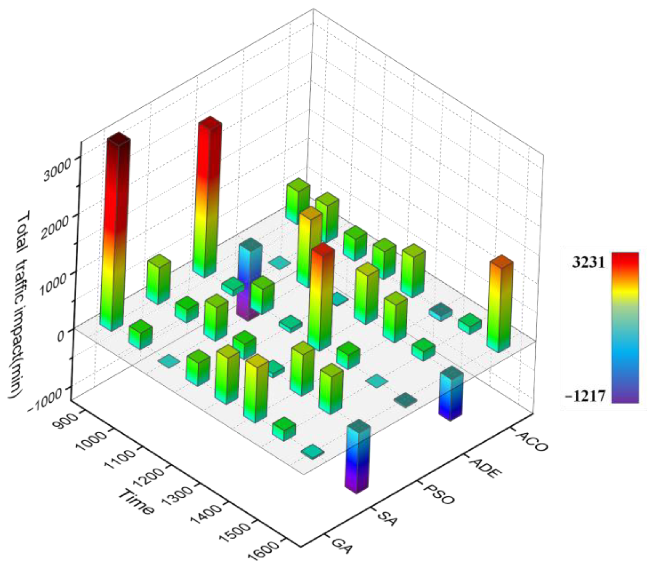
5.2. Traffic Impact Analysis

The incremental traffic impact Z(S) of different repair schedules is shown in Figure 3. At 9:00 AM, when node 70 was selected by ADE, the presence of alternative road networks around this node helped distribute the traffic more efficiently. This rerouting ability during peak traffic hours led to a significant reduction in overall travel time, as evidenced by the negative traffic impact (−1216.96). This result can be understood in the context of Braess’ Paradox, which suggests that, counterintuitively, restricting certain routes in a traffic network can lead to improved overall flow by guiding vehicles toward less congested paths [35,36]. Although node 70 remained operational, the surrounding network’s ability to absorb rerouted traffic mirrors the principles of Braess’ Paradox, where reducing available options can yield more efficient outcomes under high traffic demand. However, at 10:00 AM, when PSO also selected node 70, the traffic demand was lower, so there was less opportunity to utilize the surrounding road network effectively, resulting in a minimal traffic impact of 103.09. This demonstrates that node 70 is an optimal repair site during peak times, where traffic can reroute easily, but its advantages diminish during off-peak hours when rerouting is unnecessary or less impactful.

On the other hand, nodes like 21, 17, and 32, located in critical traffic areas, tend to cause disruptions whenever repairs are scheduled. For example, node 21 caused significant traffic disruption when selected by GA at 9:00 AM (3231.03) and by ADE at 11:00 AM (1186.28). This consistent impact highlights the importance of selecting the right time for repairs. Scheduling repairs at node 21 later in the day might be more effective in minimizing the impact, as traffic volumes typically decrease in the afternoon.

Node 17 showed a moderate impact at 12:00 PM (GA: 403.85), but when selected by PSO at 1:00 PM, the traffic impact surged to 1654.40. This suggests that node 17 may be more sensitive to traffic volumes during early afternoon hours. Minimizing repairs on node 17 during times of moderate traffic, such as the late morning or early afternoon, may reduce disruptions.

For node 32, we observe that it was selected for repairs by GA, SA, and ADE at 2:00 PM, each causing different levels of traffic disruption. GA resulted in an impact of 962.93, SA 721.25, and ADE 657.67, while PSO selected it at 9:00 AM, resulting in a significant impact of 2578.65, and ACO selected it at 4:00 PM, resulting in an impact of 1468.08. Despite the varying impact magnitudes, the afternoon time slot (2:00 PM) generally shows more manageable levels of congestion, likely due to reduced traffic demand at this time. This suggests that the algorithms strategically selected node 32 for repair when the road network could better absorb the disruption, avoiding peak traffic hours when the effects would be more severe.

It is important to acknowledge that the DTA simulation, which underpins the evaluation of road traffic resilience in this study, introduces a level of variability into the results. Since DTA is a dynamic, iterative process that simulates traffic flows based on current demand, road conditions, and network constraints, the outcomes of each simulation are not always identical. Even when no repair interventions are applied, minor variations in vehicle behavior, route choices, or traffic patterns can lead to fluctuations in total travel time.

In conclusion, by comparing how different algorithms handle key nodes like 21, 17, and 32 across various times, it becomes clear that peak-hour traffic management plays a crucial role. Scheduling repairs at node 70 during busy times (9:00 AM) is beneficial due to the presence of alternative routes, while deferring repairs on nodes like 21 and 32 to off-peak hours can help minimize traffic disruptions. A balance between node criticality and timing optimization is essential for improving overall transportation network resilience during repairs.

5.3. Computational Performance and Algorithm Selection

The computational efficiency of each optimization algorithm was assessed on a workstation equipped with an Intel Core i9-10885H processor and 32GB RAM. From the results in

Table 7. Comparison of Optimization Algorithms.

Algorithm	Total Traffic Impact (h)	Computational Time (h)	Notes
ADE	15.53	2.48	Best at minimizing traffic impact
ACO	71.72	1.59	Fast but less effective in reducing impact
SA	35.40	0.58	Fastest, but moderate impact
GA	98.47	4.23	Highest impact, longest runtime
PSO	84.57	1.88	Middle-ground performance

, we can observe significant differences in both the computational time and the total impact across the algorithms. ADE demonstrated a strong performance, achieving the lowest total impact on traffic (15.53 h), but it came at a moderate computational cost of 2.48 h. This makes ADE an excellent choice when minimizing the overall traffic impact is prioritized, although its computational time is relatively higher than algorithms like ACO and SA.

ACO performed relatively well in terms of computational efficiency, with a time cost of only 1.59 h. However, its traffic impact was considerably higher (71.72 h), making it less effective in minimizing traffic disruptions despite its lower computational requirements. SA offered the best computational efficiency with the lowest time cost (0.58 h). However, its total impact on traffic was moderate at 35.40 h. SA provides a good balance between time efficiency and traffic impact but may not outperform ADE in terms of reducing traffic disruptions. GA incurred the highest time cost (4.23 h) and also resulted in the highest total traffic impact (98.47 h). This suggests that GA was neither efficient in terms of computational time nor effective in minimizing traffic impact, making it the least favorable option among the algorithms evaluated. PSO had a moderate computational time cost of 1.88 h but showed a high traffic impact of 84.57 h. This positions PSO as a middle-ground algorithm in terms of computational efficiency but relatively ineffective in reducing traffic impact.

Given these trade-offs, different optimization algorithms are suitable for different urban repair planning scenarios:

• ADE is the best choice when the primary goal is to minimize traffic impact, making it ideal for large-scale infrastructure repair planning;
• SA is optimal for real-time applications requiring fast decision-making due to its superior computational efficiency;
• ACO provides a balanced approach, performing well in scenarios where both computational efficiency and impact reduction are important;
• GA and PSO are less effective for large-scale urban repair scheduling, as they exhibit high traffic impact and prolonged computation times.

These insights provide practical guidance for urban planners and infrastructure managers in selecting the most suitable optimization strategy based on specific constraints.

6. Conclusions

This study introduces a novel bi-level optimization framework for coordinating water supply network repairs with the resilience of the transportation network, leveraging a DTA model. By integrating the scheduling of infrastructure repairs and dynamically assessing their impact on traffic, this approach allows for minimizing disruptions in two critical urban systems. The framework effectively captures the interdependencies between water supply and road networks, providing actionable insights for urban infrastructure management.

The results demonstrate that optimizing the timing and location of repairs significantly mitigates the negative impact on traffic flow, especially during peak hours. For instance, repairing key nodes, such as node 70, during peak hours showed reduced travel time by efficiently redistributing traffic across alternative routes. In contrast, repairs at critical nodes, such as 21 and 17, caused substantial disruptions, highlighting the importance of carefully selecting repair schedules based on real-time traffic demand.

Among the optimization algorithms tested, ADE consistently achieved the lowest total traffic impact, making it the most effective in terms of resilience enhancement. While SA offered superior computational efficiency, it was less effective in minimizing traffic disruptions compared to ADE. Algorithms like GA and PSO showed mixed results, with GA being the least effective in both minimizing traffic disruptions and computation time. These findings emphasize the importance of selecting the right algorithm based on the specific priorities of the optimization task—whether minimizing impact or reducing computation time.

In summary, this research highlights the importance of integrating water supply network maintenance with dynamic traffic management to achieve a resilient urban infrastructure. The bi-level optimization model offers a practical tool for urban planners and policymakers, enabling them to make informed decisions about repair scheduling and resource allocation. Future work could extend this framework by incorporating real-time data from sensors and IoT devices, allowing for adaptive, real-time optimization that responds dynamically to evolving traffic conditions and repair needs. Additionally, exploring the environmental and economic impacts of repair schedules would further enhance the model’s applicability to broader sustainability goals.

References

- Buldyrev, S.V.; Parshani, R.; Paul, G.; Stanley, H.E.; Havlin, S. Catastrophic cascade of failures in interdependent networks. Nature 2010, 464, 1025–1028. [Google Scholar] [CrossRef] [PubMed]
- Gursan, C.; de Gooyert, V.; de Bruijne, M.; Rouwette, E. Socio-technical infrastructure interdependencies and their implications for urban sustainability; recent insights from the Netherlands. Cities 2023, 140, 10439. [Google Scholar] [CrossRef]
- Wang, N.; Jin, Z.-Y.; Zhao, J. Cascading failures of overload behaviors on interdependent networks. Phys. A Stat. Mech. Its Appl. 2021, 574, 125989. [Google Scholar] [CrossRef]
- Wert, J.L.; Shetye, K.S.; Li, H.; Yeo, J.H.; Xu, X.; Meitiv, A.; Xu, Y.; Overbye, T.J. Coupled Infrastructure Simulation of Electric Grid and Transportation Networks. In Proceedings of the 2021 IEEE Power & Energy Society Innovative Smart Grid Technologies Conference, Washington, DC, USA, 16–18 February 2021. [Google Scholar]
- Kuliczkowska, E. The interaction between road traffic safety and the condition of sewers laid under roads. Transp. Res. Part D-Transp. Environ. 2016, 48, 203–213. [Google Scholar] [CrossRef]
- Rinaldi, S.M.; Peerenboom, J.; Kelly, T.K. Identifying, understanding, and analyzing critical infrastructure interdependencies. Control Syst. IEEE 2002, 21, 11–25. [Google Scholar] [CrossRef]
- Imani, M.; Hajializadeh, D. A resilience assessment framework for critical infrastructure networks’ interdependencies. Water Sci. Technol. 2019, 81, 1420–1431. [Google Scholar] [CrossRef]
- Ozdemir, Z.; Coulier, P.; Lak, M.A.; Francois, S.; Lombaert, G.; Degrande, G. Numerical evaluation of the dynamic response of pipelines to vibrations induced by the operation of a pavement breaker. Soil Dyn. Earthq. Eng. 2013, 44, 153–167. [Google Scholar] [CrossRef]
- Wang, W.; Robert, D.J.; Zhou, A.; Li, C.Q.; Wasim, M. Full Scale Corrosion Test on Buried Cast Iron Pipes. In Proceedings of the Fourth International Conference on Sustainable Construction Materials and Technologies, Las Vegas, NV, USA, 7–11 August 2016. [Google Scholar]
- Jayasinghe, P.A.; Derrible, S.; Kattan, L. Interdependencies between Urban Transport, Water, and Solid Waste Infrastructure Systems. Infrastructures 2023, 8, 76. [Google Scholar] [CrossRef]
- Uddin, S. Interdependency Between Water and Road Infrastructures: Cases and Impacts. Ph.D. Thesis, University of South Florida, Tampa, FL, USA, 2023. [Google Scholar]
- El-Zahab, S.; Zayed, T. Leak detection in water distribution networks: An introductory overview. Smart Water 2019, 4, 5. [Google Scholar] [CrossRef]
- Underground Pipeline Committee of CACP. Statistical Analysis Report of Underground Pipeline Accidents in China in 2021; “Pipeline Accident” WeChat Official Account, 22 January 2022. Available online: https://mp.weixin.qq.com/s/yWbAwD1aTfPTG_Whre0Ajg (accessed on 11 March 2025).
- Mottahedin, A.; Giudicianni, C.; Cunha, M.C.; Creaco, E. Multiobjective Approach for Water Distribution Network Design Combining Pipe Sizing and Isolation Valve Placement. J. Water Resour. Plan. Manag. 2024, 150, 04024043. [Google Scholar] [CrossRef]
- Ramani, K.; Rudraswamy, G.K.; Umamahesh, N.V. Optimal Design of Intermittent Water Distribution Network Considering Network Resilience and Equity in Water Supply. Water 2023, 15, 3265. [Google Scholar] [CrossRef]
- Chu, J.; Wang, H.; Shao, Y.; Yu, T. Analysis on theory and technical framework of optimal maintenance of water supply network. Water Resour. Prot. 2022, 38, 67–72. [Google Scholar]
- Atat, R.; Ismail, M.; Serpedin, E. Cascading Failures Mitigation Strategy for Resilient Water Infrastructures*. IFAC-Pap. 2023, 56, 4645–4650. [Google Scholar] [CrossRef]
- Prasad, T.D.; Park, N.-S. Multiobjective Genetic Algorithms for Design of Water Distribution Networks. J. Water Resour. Plan. Manag. 2004, 130, 73–82. [Google Scholar] [CrossRef]
- Farmani, R.; Kakoudakis, K.; Behzadian, K.; Butler, D. Pipe Failure Prediction in Water Distribution Systems Considering Static and Dynamic Factors. Procedia Eng. 2017, 186, 117–126. [Google Scholar] [CrossRef]
- Marshall, N.L. Forecasting the impossible: The status quo of estimating traffic flows with static traffic assignment and the future of dynamic traffic assignment. Res. Transp. Bus. Manag. 2018, 29, 85–92. [Google Scholar] [CrossRef]
- Kachroo, P.; Özbay, K.M.A. Traffic Assignment: A Survey of Mathematical Models and Techniques. In Feedback Control Theory for Dynamic Traffic Assignment; Kachroo, P., Özbay, K.M.A., Eds.; Springer International Publishing: Cham, Switzerland, 2018; pp. 25–53. [Google Scholar]
- Hu, Q.; Che, D.; Wang, F.; He, L. Analyzing the effects of extreme cold waves on urban water supply network safety: A case study from 2020 to 2021. Urban Clim. 2024, 58, 102146. [Google Scholar] [CrossRef]
- Zhou, X.; Taylor, J. DTALite: A queue-based mesoscopic traffic simulator for fast model evaluation and calibration. Cogent Eng. 2014, 1, 961345. [Google Scholar] [CrossRef]
- US Bureau of Public Roads Office of Planning. Traffic Assignment Manual for Application with a Large, High Speed Computer; US Department of Commerce: Washington, DC, USA, 1964.
- Agency, F.E.M. Hazus Earthquake Model Technical Manual; FEMA: Hyattsville, MD, USA, 2022. [Google Scholar]
- Zhang, J.; Sanderson, A.C. Adaptive Differential Evolution; Springer: Berlin/Heidelberg, Germany, 2009. [Google Scholar]
- Holland, J.H. Genetic algorithms. Sci. Am. 1992, 267, 66–73. [Google Scholar] [CrossRef]
- Kennedy, J.; Eberhart, R. Particle swarm optimization. In Proceedings of the ICNN’95 International Conference on Neural Networks, Perth, Australia, 27 November–1 December 1995; Volume 1944, pp. 1942–1948. [Google Scholar]
- Bertsimas, D.; Tsitsiklis, J. Simulated annealing. Stat. Sci. 1993, 8, 10–15. [Google Scholar] [CrossRef]
- Dorigo, M.; Maniezzo, V.; Colorni, A. Ant sytem: Optimization by a colony of cooperating agents. IEEE Trans. Syst. Man Cybern.-Part B Cybern. 1996, 26, 29–41. [Google Scholar] [CrossRef] [PubMed]
- Adrian, A.M.; Utamima, A.; Wang, K.-J. A comparative study of GA, PSO and ACO for solving construction site layout optimization. KSCE J. Civ. Eng. 2015, 19, 520–527. [Google Scholar] [CrossRef]
- Papazoglou, G.; Biskas, P. Review and Comparison of Genetic Algorithm and Particle Swarm Optimization in the Optimal Power Flow Problem. Energies 2023, 16, 1152. [Google Scholar] [CrossRef]
- Misra, B.; Chakraborty, S. Ant Colony Optimization—Recent Variants, Application and Perspectives. In Applications of Ant Colony Optimization and Its Variants: Case Studies and New Developments; Dey, N., Ed.; Springer Nature: Singapore, 2024; pp. 1–17. [Google Scholar]
- Musa, R.; Chen, F.F. Simulated annealing and ant colony optimization algorithms for the dynamic throughput maximization problem. Int. J. Adv. Manuf. Technol. 2008, 37, 837–850. [Google Scholar] [CrossRef]
- Braess, D.; Nagurney, A.; Wakolbinger, T. On a paradox of traffic planning. Transp. Sci. 2005, 39, 446–450. [Google Scholar] [CrossRef]
- Lin, J.; Hu, Q.; Jiang, Y. Braess Paradox in Optimal Multiperiod Resource-Constrained Restoration Scheduling Problem. Int. J. Civ. Eng. 2024, 22, 1321–1338. [Google Scholar] [CrossRef]