Streamflow Measurements Using an Underwater Acoustic-Based Approach: A Case Study in a Shallow Narrow Silt-Bed River

Abstract

The recent improvements in streamflow measurement approaches have boosted the reliability and accuracy of river flow measurement. In this study, long-term measurements of river discharge in the Tokoro River, Japan, were conducted. The key objective of this work is to investigate the extent of river flow measurement in a very shallow and narrow silt stream using the fluvial acoustic tomography system (FAT). Despite the preliminary nature of the measurement results, the recorded data were subject to analysis from three different outlooks. First, examinations were performed under very shallow and high-water conditions. Second, examinations were performed using double acoustic frequency. Third, examinations were performed using multiple independent flow datasets. As a new achievement in terms of advanced monitoring capabilities, it was documented that the measurement by the FAT was possible even in extremely shallow conditions. However, the minimum water depth along the measured cross-section must be ≥9 cm. Moreover, the FAT system demonstrated its capability to monitor streamflow in high water levels. In addition, it was found that using high transmission frequency can provide shorter wavelengths, permitting better spatial resolution and higher velocity resolutions and hence desirable measurement accuracy. Nevertheless, measurements in the presence of high suspended sediment particles were lacking. Alternatively, a lower transmission frequency offers a longer wavelength, which might be less sensitive to small-scale variations and results in an imprecise degree of measurements. Nonetheless, measurements can be accomplished even during the mobilization of a high concentration of suspended sediment matters. Finally, using multiple independent streamflow measurement records, the results proved that the flow measured by the FAT system was in very good agreement with the records acquired using sophisticated measurement approaches such as HADCP and STIV with a very low range of uncertainty.

1. Introduction

In comparison to other areas in the Japanese Archipelago, the Okhotsk Region in Hokkaidō Island experiences a subarctic climate characterized by long cold winters and shorter cooler summers, which creates unique hydrological features. According to the Japanese Meteorological Agency, the Okhotsk Region experiences the least amount of rainfall nationwide; nonetheless, the region is not immune to flood events. For example, in 2016, a record-breaking flood occurred as a result of prolonged moderate-to-heavy rainfall events as a result of three typhoons occurring in a single week [1,2]. Therefore, the accurate and advanced monitoring of river flow dynamics is an essential challenge, even in cold climate regions.

Nonetheless, river watersheds in the Okhotsk Region are still pristine and largely untouched by human interference. Moreover, the majority of the rivers in the region are characterized by their shallower and narrower stream channels. Basically, streamflow measurement in this region is estimated using the traditional method, namely the rating curve (RC) approach. In simple words, this method is based on the existence of a relationship between the water level (H) and river discharge (Q); therefore, in the literature, it is sometimes termed as the (H-Q) approach. Yet, streamflow measurement by means of the RC approach poses two key challenges for providing reliable estimates. First, in Hokkaidō, the freezing season takes place between late December and early April, with an approximate period of 100 days per year. Unlike other seasons, the relationship between the water level and river flow during freezing seasons is unique, since the temporal variation in water level is a function of three key terms, namely (i) riverbed height, (ii) effective depth, and (iii) the draft depth of river ice [3]. Consequently, developing a year-round RC equation or multiple equations would not be practical in the long term, as the empirical parameters change continuously. Second, during warm weather circumstances, river flow under low flow-conditions is steady; accordingly, the application of the RC approach is appropriate. Nevertheless, it is essential to take into account that the region is susceptible to floods induced by seasonal typhoons as well as tropical cyclones. In the case of high-flow conditions, which is an important target to be investigated, the evaluated streamflow by means of the RC is questionable and unreliable in many cases. Past works [4,5,6,7,8] have pointed out that substantial uncertainties in streamflow measurements estimated by a modeled RC equation may arise due to several difficulties and/ or errors, including (i) errors in stage measurement [4], (ii) errors in interpolation and extrapolation in the established RC relationship [4,6], and (iii) changes in the channel cross-section due to unrecognized fill/scour, ice, vegetation, backwater, and hysteresis effects, which needed to be considered in the calibration of the RC parameters [7,8]. Therefore, there is a crucial necessity for utilizing another reliable streamflow measurement approach other than the RC.

Shedding light on streamflow measurement methods, the literature contains numerous works that discuss the potential of recent streamflow measurement approaches. Nonetheless, it is important to bear in mind that every streamflow measurement approach has a unique set of capabilities and some drawbacks that cannot be avoided in some cases mainly due to site-related features and limitations. For example, acoustic Doppler current profiler (ADCP) instruments themselves are expensive. Moreover, they face deployment restrictions in some locations on river sites and pose risks to the operators during flood conditions. More importantly, operating ADCPs need experienced hands, as site-related parameters should be inputted carefully [9,10,11]. Considering the large-scale particle image velocimetry (LSPIV) approach as another measurement alternative, it should be acknowledged that this technique has several benefits [12,13], but some limitations have been reported. For example, a key shortcoming of LSPIV is that velocity components cannot be determined if the angle is less than 15 degrees from the horizontal [14]. In addition, the accuracy of the LSPIV estimates can be affected by high winds, as well as bank vegetation, which may limit the view of the monitored field. Also, this approach is also not robust at night or when ice is limiting the camera’s view of the stream water surface [15]. In order to improve the measurement accuracy of streamflow and perform a long-term assessment of river flow dynamics in the region, a long-term monitoring program by Hokkaisuikō Consultant Corporation, Hokkaidō, Japan. in the Tokoro River was started. At the first stage, continuous measurements of streamflow using two key advanced approaches were used, namely (i) the horizontal acoustic Doppler current profiler (HADCP) and (ii) space–time image velocimetry (STIV) using an infrared camera. However, a notable difference among the records acquired by the HADCP, STIV, and RC was observed. At a later stage, the underwater acoustic tomography system (FAT) was introduced, aiming to provide another independent measurement record.

The characteristics of the current studied site (i.e., Tokoro River) are totally different compared to the implemented past project utilizing the FAT system [16]. In other words, this observation program was performed in one of the coldest regions in East Asia in a shallow and narrow silt-bed stream that carries high quantities of sediment matter and debris. Taking into account that large concentrations of sediment particles can significantly impact the performance of flow monitoring using acoustic approaches, it is necessary to consider the extent of the measurement ability of acoustic-based approaches [17]. In order to overcome the difficulties related to the strong attenuation of the acoustic signals in high-turbidity conditions, the current monitoring program by the FAT system was implemented using two central frequencies.

Therefore, the goal of this study is to present and discuss the key potentials and challenges encountered during the field observation program to provide accurate streamflow measurements in the Tokoro River located in the Okhotsk Region. This study is motivated by the need to rigorously evaluate the performance of underwater acoustics as a streamflow measurement approach, particularly in comparison to established independent techniques. While our main target was to increase the accuracy of the measured river discharge, the scope of this study will be focused on measurements acquired using an underwater acoustic system hereinafter referred to as the Fluvial Acoustic Tomography System (FAT) under low- and high-flow conditions, as well as in high-turbid-flow conditions. One of the main novelties of the current study resides in using double frequency to provide continuous monitoring of streamflow dynamics. Hence, the contribution of this work is to fill a gap in acoustic monitoring behavior in a river channel that carries a high amount of sediment loads within narrow-stream conditions.

2. Materials and Methods

2.1. Study Site

Field measurements were carried out in the Tokoro River, which is the largest river in the Okhotsk Region of Japan located in Kitami City of the Hokkaidō prefecture (Figure 1). The river channel is 120 km in length, with an average width of 40 m near the observation site, and it has a basin area of 1930 km². The river originates from the Mikuni Mountain, passes through Oketo and Kunneppu towns, respectively, then merges with its main tributary, i.e., Muka River in the center of Kitami city, before it pours into the Okhotsk Sea. The region is characterized by a humid continental climate with cold winters and relatively warm summers. The coldest months are January and February, with an average low temperature of −9 °C, and the warmest month is August, with an average high temperature of 20 °C. The average annual rainfall is approximately 800 mm, where the wettest month is August and the driest month is February.

Presented in Figure 1b are the positions of the measurement instruments that were used in this monitoring program. The Kamikawazoi Station measures the water level hourly; thus, the streamflow (Q_RC) was continuously estimated using an empirical rating curve equation derived for this site. The estimated annual mean discharge was 35 m³/s.

The horizontal acoustic Doppler profiler (HADCP) sensor was mounted on the left bank to provide discharge records (Q_HADCP). It is noteworthy that the frequency of the used HADCP was 300 kHz. In addition, an infrared camera (FLIR FC-series 0) was mounted ~ 60 m from the river’s left bank to provide river flow estimates based on an approach called (space–time image velocimetry or alternatively, STIV). Finally, measurements by means of the FAT system were carried out using two pairs of omnidirectional acoustic transducers (T226, Neptune Sonar Ltd., East Yorkshire, UK) and (T257, Neptune Sonar Ltd.) operated using a central frequency of 58 kHz and 30 kHz, respectively. Both transducers (T226 and T257) were placed side by side on both riverbanks upstream to the measurement site at S1 and S2 depicted in Figure 1b and Figure 2. The oblique distance between the left bank transducer and the right bank one was measured as (L = 85 m) using a total station, shown in Figure 1b. In this context, it is important to point out that the FAT system in its current version can work using three different frequencies as follows: (i) 58 kHz, which is preferred for shallow and narrow streams; (ii) 30 kHz, suitable for wide stream channels; and (iii) 17 kHz, which is suitable for coastal areas. Fundamentally, the measurements were planned to be performed using the 58 kHz frequency. This is because high transmission frequencies give precise estimates in the case of narrow and shallow stream channels [16]. However, in high-turbidity conditions, it was found that a strong attenuation of the acoustic signal occurred. Hence, at a later stage, it was decided to carry out double frequency measurements using the 30 kHz transducers. In addition, according to the guidelines proposed in [18], it was stated that the placement of acoustic transducers should be essentially in a diagonal plane to improve the quality of the measured acoustic signals and minimize unacceptable uncertainties in streamflow determination.

2.2. FAT Measurement Principles

As mentioned earlier, in this research, the main concentration is directed to streamflow measurement using the FAT system. The basic principle of measurement using the FAT system is the travel time approach [19]. To clarify, each transducer transmits acoustic pulses to the counterpart transducer at certain times predefined using GPS satellites concurrently. At the same time, each transducer receives the transmitted signals from the opposite transducer. Also, the transmission rate was set to every 30 s. Therefore, for a certain time (e.g., 1 July 2024 14:30:30), it can be said that t₁ is the elapsed time for an acoustic pulse transmitted from S1 and received at S2. In the same manner, t₂ is the elapsed time for an acoustic pulse triggered from S2 and received at S1. As a result, the stream cross-sectional average velocity (U) along the transmission line (S1–S2) can be computed as

$$U={\displaystyle \frac{L}{2}} \left({\displaystyle \frac{1}{t_1}}-{\displaystyle \frac{1}{t_2}}\right)$$

(1)

where L is the length of the distance between S1 and S2. Accordingly, the streamwise cross-sectional average velocity component (V) can be expressed using Equation (2) as

$$V={\displaystyle \frac{U}{\cos \theta }}$$

(2)

where $\theta$ is the angle between the transmission line, and the streamwise mean current direction (Figure 1b) was determined using ADCP boat data. As a result, the river discharge (Q_FAT) can be estimated using the fundamental flow equation in open channels as

$$Q_{FAT}=V\times A\times \sin \theta$$

(3)

where A is the cross-sectional area formed between S1 and S2. To provide continuous measurement of the cross-sectional area along S1–S2, the longitudinal and latitudinal information of the river cross-section was measured using a total station. On the other hand, the mean water level was continuously measured using a pressure transducer; therefore, the integration between the horizontal line of the water surface elevation and the river cross-section curve gives the precise value of the cross-sectional area.

As previously mentioned, in this monitoring program, we used two types of transducers, each of which transmits acoustic signals using 58 kHz and 30 kHz, central frequencies, respectively, as shown in Figure 2c,d. The main reason for this combination was to obtain measurements by means of the FAT system in very high concentrations of sediment flux. The 58 kHz transducers were placed above the riverbed by ~25 cm, whereas the 30 kHz transducers were placed above the riverbed by ~40 cm.

3. Results

Figure 3 shows the temporal variations in the water level recorded at Kamikawazoi Station during some events in 2023 and 2024. During these periods, the FAT system was deployed at the studied site and long-term observation started. First, in 2023, river flow measurements using the 58 kHz frequency of the FAT system, as well as measurements using both the HADCP and an infrared camera, were performed. Then, all monitoring systems were uninstalled before the winter season came, as the installations were not designed to be sustained during extreme cold temperatures (i.e., less than −20 °C). Again, in 2024, flow measurement using the same FAT 58 kHz was carried out; however, one pair of the 30 kHz transducers was joined to the existing 58 kHz transducers to provide additional records in the case of higher sediment flux triggered during rainy events.

To narrow the scope of this study to events of significance, flow measurements were investigated across three different circumstances as follows: (i) streamflow measurement in very shallow- and high-flow conditions, (ii) streamflow measurements using double frequency, and (iii) streamflow comparison using other independent streamflow records.

3.1. Flow Measurement in Very Shallow- and High-Flow Conditions

Figure 4a shows the temporal variations in the water level at Kamaikawazoi Station in case#1, i.e., very shallow-flow conditions, as well as case#2, i.e., in high-flow conditions, respectively.

First, we must shed light on the measurements in shallow-flow conditions as plotted in case#1. It can be seen in Figure 4a that the water level rose from approximately 2.16 m and peaked at 2.58 m. Nevertheless, it can be noticed that measurement by means of the FAT system was applicable as the water level exceeded ~2.2 m, as illustrated in Figure 4a–c. The temporal variations in the streamflow obtained by Q_FAT and Q_RC were plotted in Figure 4c. Unfortunately, during the peak of this event, some acoustic signals could not be received in some periods. In addition, in very low-flow conditions, considerable variation between the Q_FAT and Q_RC can be detected. However, this variation was very insignificant as the water level rose (Figure 4a–c). Moreover, to give a sensible comparison of the flow records estimated by the FAT system, the uncertainty was estimated using the percentage error as given in Equation (4).

$$\mathrm{U}\mathrm{n}\mathrm{c}\mathrm{e}\mathrm{r}\mathrm{t}\mathrm{a}\mathrm{i}\mathrm{n}\mathrm{t}\mathrm{y}={\displaystyle \frac{Q_{RC}-Q_{FAT}}{Q_{FAT}}} (\%)$$

(4)

Apparently, the plotted uncertainty in Figure 4d shows that measurement by FAT was underestimated in low-flow conditions; however, these variations became very low as the water level increased.

Examining the measurement in high-flow conditions as depicted in case#2, it can be noted that the water level started to rise from 2.1 m and peaked at 5.1 m (Figure 4a). During the rising portion, it can be found that the majority of the signals could not be analyzed because the SNR values were very low, as documented in Figure 4e. The cross-sectional average velocity had an approximate range of 0.45 ~ 1.1 m/s. Encouragingly, the temporal variations in the flow estimated between Q_FAT and Q_RC were in very good agreement (Figure 4c), with a mean range of uncertainty that can be estimated as ± 17%, as presented in Figure 4d.

3.2. Flow Measurement Using Double Frequency

In the same manner, Figure 5a presents the temporal variations in the water level acquired at Kamikawazoi Station in both case#3 and case#4, respectively. As can be seen in Figure 5a, the water level at Kamikawazoi Station in these two cases did not increase as much as in case#2.

In case#3, it can be noticed that the FAT 58 kHz system started to capture the mean velocity and river flow at the beginning of the rising area, as revealed in Figure 5b,c. However, the system shutdown due to battery failure since the late night of 28 August and was resolved at noon on 30 August. Alternatively, in the case of the FAT 30 kHz, it should be mentioned that the measurement was possible if the water level exceeded ~2.6 m. In addition, to save the system energy and avoid frequent battery replacement, the FAT system was scheduled to boot up automatically on 28 August at 12:00 p.m. Accordingly, it can be seen that the cross-sectional average velocity and discharge were recorded since the scheduled time. In general, the flow comparison between the FAT systems and the counterpart records obtained by Kamikawazoi Station were very comparable, as depicted in Figure 5c,d.

Case#4, on the other hand, shows that the water level at Kamikawazoi Station peaked at 3.9 m. It can be realized in Figure 5e that the received SNR signals of the FAT 58 kHz system dropped down during the rising part, especially in the case of the signals received at the upstream transducer. Likewise, the received SNR signals of the FAT 30 kHz exhibited similar behavior with less transmission loss in comparison to the FAT 58 kHz. The cross-sectional mean velocity as measured by FAT 58 kHz (black) and FAT 30 kHz (blue) were in good agreement. Nevertheless, the velocity measured by FAT 58 kHz showed a slight increase during the end of the flood event (Figure 5b). This maybe induced by some unstable SNR signals obtained by the downstream transducer (Figure 5e). As a result, the uncertainty between the FAT records and the streamflow records estimated at Kamikawazoi Station was comparable, as depicted in Figure 5d.

3.3. Flow Measurement Using Multiple Independent Streamflow Records

It is well known that the streamflow measurements by means of the RC approach could be imprecise in some periods, particularly in high-flow conditions. Therefore, to offer more reliable and obvious insights on the river flow records, additional flow records by means of the HADCP and STIV conducted in 2023 were revealed in Figure 6 as case#5 and case#6, respectively. In this regard, it is very important to mention that measurements by means of the HADCP were possible if the water level at Kamikawazoi Station exceeded ~2.7 m. On the other hand, STIV flow measurement was performed if the water level at Kamikawazoi Station surpassed ~4.2 m.

As shown in Figure 6a, the water level at Kamikawazoi Station peaked at 4.49 m and 5.53 m in case#5 and case#6, respectively. The cross-sectional average velocity in case#5 ranged between 0.85 m/s and 1.3 m/s, approximately. Similarly, the cross-sectional mean velocity in case#6 ranged between 0.95 m/s and 1.48 m/s. Taking into account the streamflow records presented in Figure 6c, two significant points can be detected. First, in the case of high-water levels, i.e., in both case#5 and case#6, the flow records obtained by means of the RC approach were overestimated in comparison to the HADCP, FAT, and STIV, as depicted in case#5. This overestimation was even greater in case#6. On the other hand, as the water level decreases, the flow record obtained by means of the RC approach agreed with the other flow records. Of great importance in this context, it can be seen that flow recorded by the FAT system offered very comparable records in line with the other advanced approaches (i.e., STIV and HADCP). Furthermore, the mean uncertainty of the Q_FAT vs. Q_HADCP and Q_FAT vs. Q_STIV was ± 15%, approximately. Unfortunately, in case#6, the battery of the FAT system was depleted by 18 September and river flow could not completely be measured for the whole event.

4. Discussion

Past works have shown successful examples of river flow dynamics monitoring using underwater acoustic tomography, i.e., the FAT system. For example, a previous study performed a comprehensive assessment of streamflow records using high-resolution data obtained using the FAT system. The assessment findings demonstrated that streamflow records obtained in high temporal resolution in real-time could increase the ability to monitor the short-term fluctuations of floods [20]. Although the results presented from this observation program are preliminary, several important findings can be discussed.

4.1. Inferences of River Flow Measurement in Very Shallow- and High-Flow Conditions

Falvey [21] pointed out that the water surface of a river can be considered as a perfect reflector of acoustic signals. More importantly, the condition for a smooth water surface reflector can be expressed using Equation (5) as

$$\mathrm{\lambda }=8\times h\times \sin \phi$$

(5)

where $\lambda$ is the wavelength of an acoustic wave, h is the minimum water depth, and $\phi$ is the grazing angle of an acoustic wave made with a water surface, being at least 1°. In the case of riverbeds, the prediction of acoustic wave reflection behavior is quite complex because riverbed materials are diverse. However, it can be stated that the reflection of acoustic signals from the riverbed is highly attenuated. Taking into account that the sound speed in freshwater c is 1481 m/s and the transducer frequency is f = 58 kHz, the wavelength according to Equation (6) is 2.5 cm.

$$\mathrm{\lambda }={\displaystyle \frac{c}{f}}$$

(6)

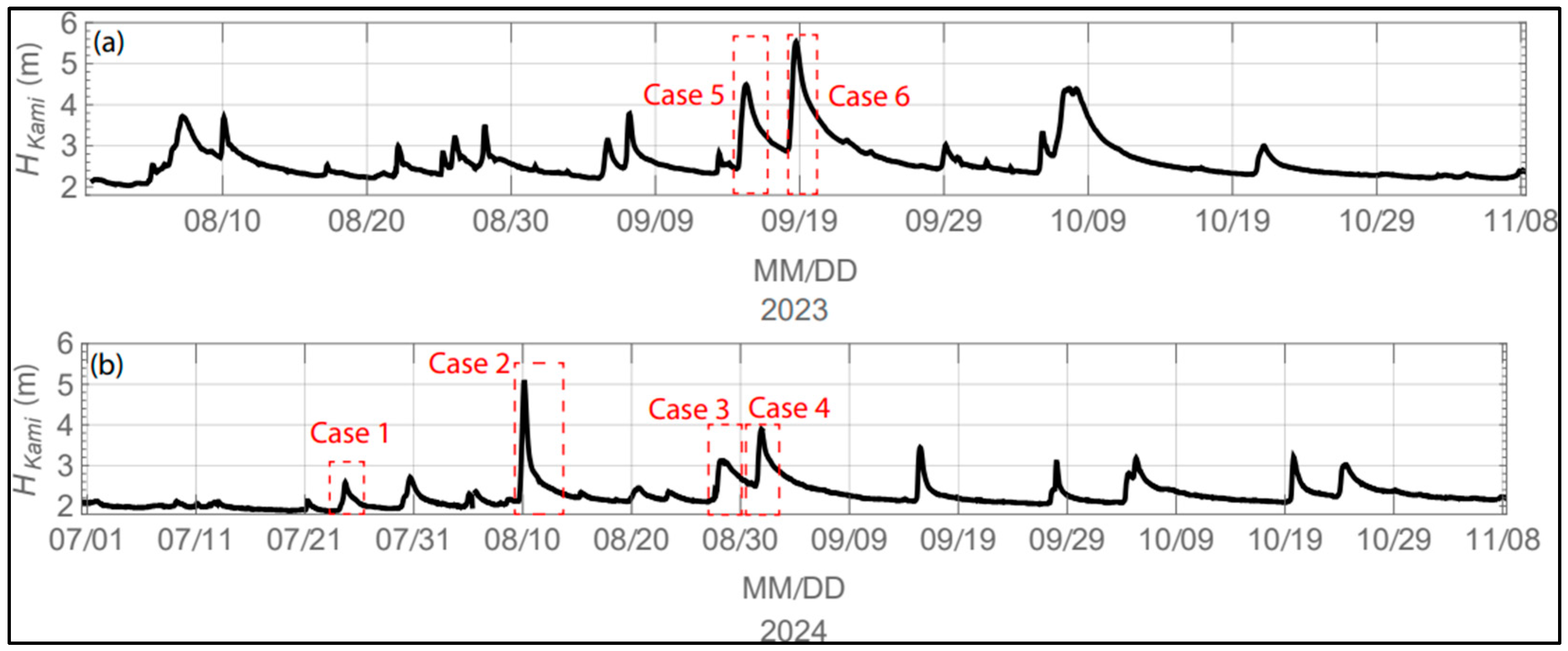
As a result, substituting in Equation (5), it can be found that the minimum water depth (h) should be at least ~18 cm. As a result, it can be understood why the transducers of 58 kHz and 30 kHz systems were placed above the riverbed by ~25 cm and ~40 cm, respectively. In shallow water levels, as presented in case#1 (Figure 4), it was observed that the river flow estimated by the FAT system was underestimated compared to the flow estimated using the RC approach computed at Kamikawazoi Station. 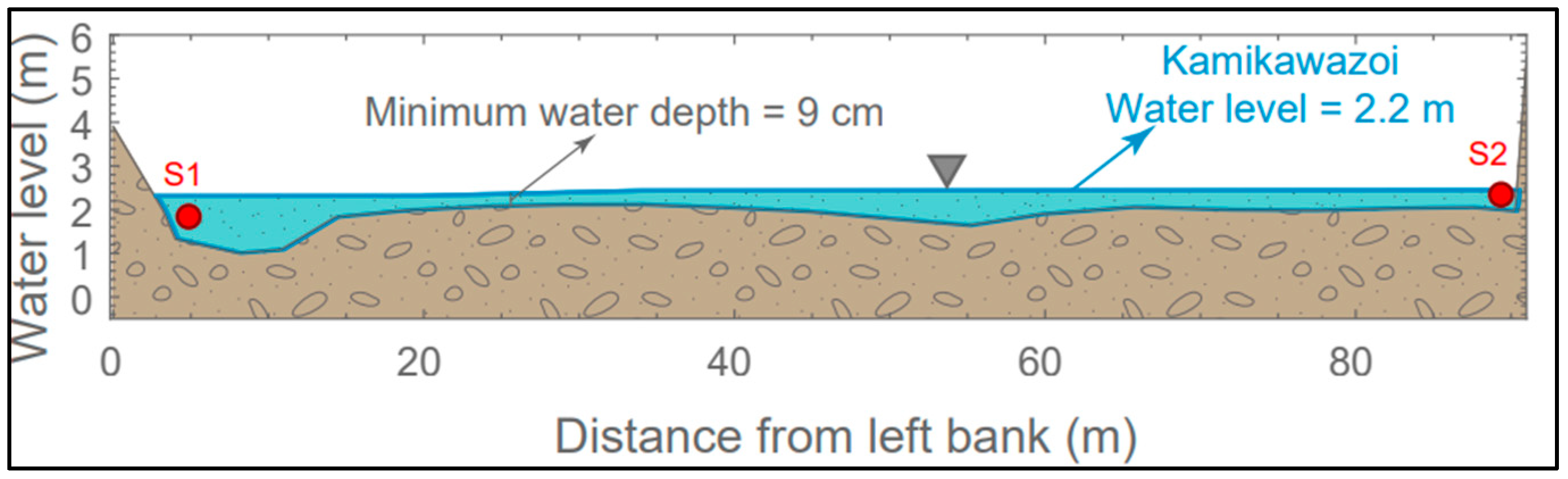However, the agreement between Q_FAT and Q_RC became higher as the water level at Kamikawazoi Station exceeded ~2.5 m, as shown in Figure 4a–c. In this context, it is crucial to recall that the FAT system started to provide acoustic measurements when the water level at Kamikawazoi Station exceeded 2.2 m. At this level strictly, the minimum water depth along the transmission line was measured as 9 cm, as depicted in Figure 7, which was half of the minimum wave height (i.e., ~18 cm). This finding demonstrates the ability of the FAT 58 kHz to provide measurements at this depth. Nevertheless, the accuracy of the measurement should be verified with another robust measurement approach (i.e., other than the RC approach), because it can be seen in case#1, Figure 4c,d, that the FAT system measurements underestimated under this extremely shallow depth.

Alternatively, in high water levels, as presented in case#2, it can be seen that the FAT system demonstrated the capability to measure river flow. The key question in this context is measurement by the FAT limited up to a certain high-water depth or during either rising or falling limbs? The answer to this question is simply no. In other words, it can be seen in case#2 that unlike in the rising portion, the river discharge was perfectly measured by the FAT system during the falling portion regardless of the water level (Figure 4c). In addition, it can be verified in case#6 that the water level was greater than in the event observed in case#2. 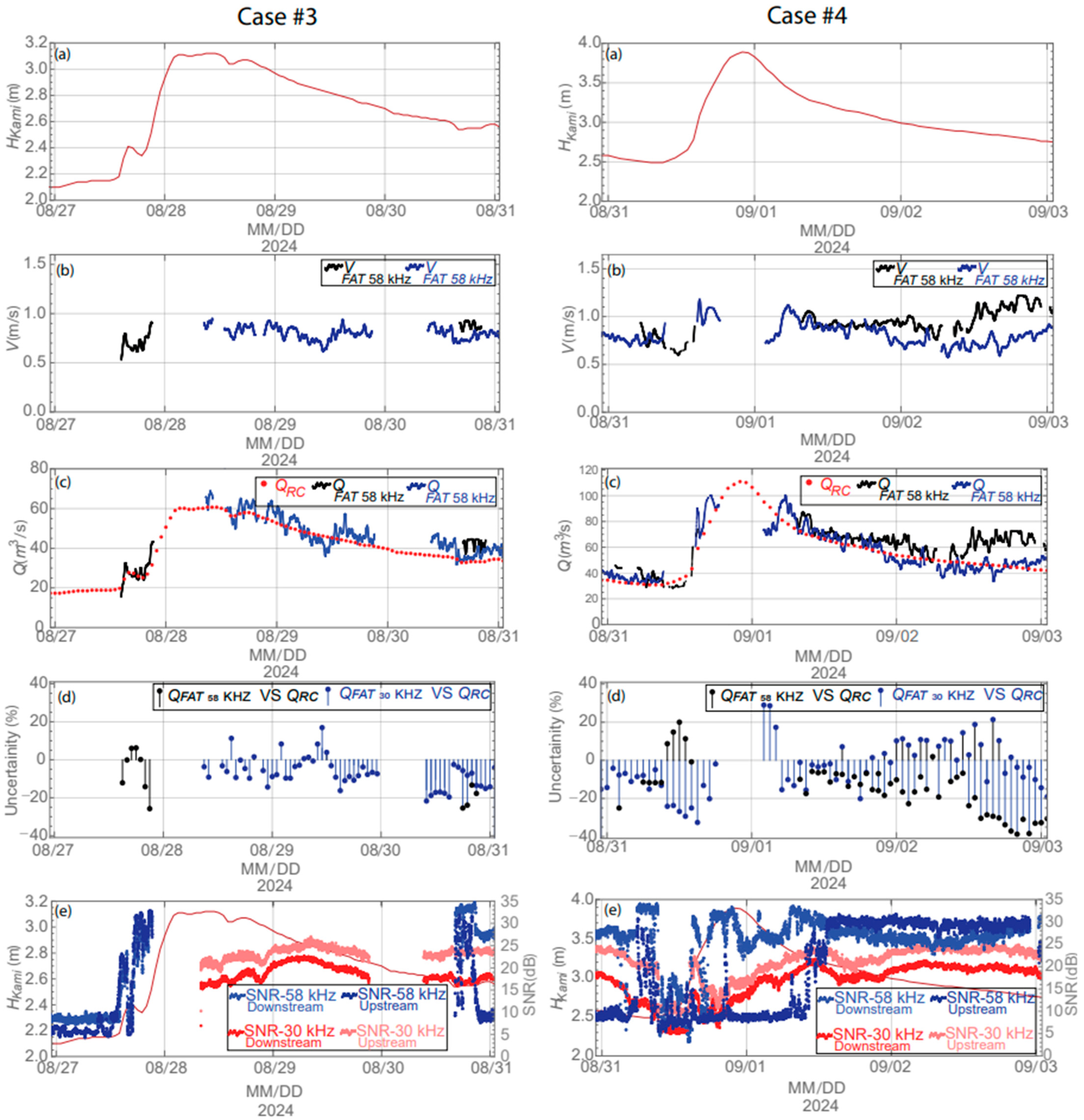The streamflow by the FAT system was also captured during the rising portion of that event, as depicted in Figure 6c. However, the discontinuity in the streamflow measurements was mainly interrupted owing to the fact that the SNR signals recorded by the FAT system dramatically dropped down, as revealed in Figure 4e. The key reason for this decline can be attributed to the mobilization of high concentrations of sediment matter that attenuated the strength of the recorded acoustic pulses between the transducers. For example, Figure 8 documents the high-turbid condition of the river site triggered by a very mild rainy event. Remarkably, the water level measured at Kamikawazoi Station at that time was 1.91 m, and the total daily rainfall recorded was ~2 mm.

4.2. Inferences of River Flow Measurement Using Double Frequency

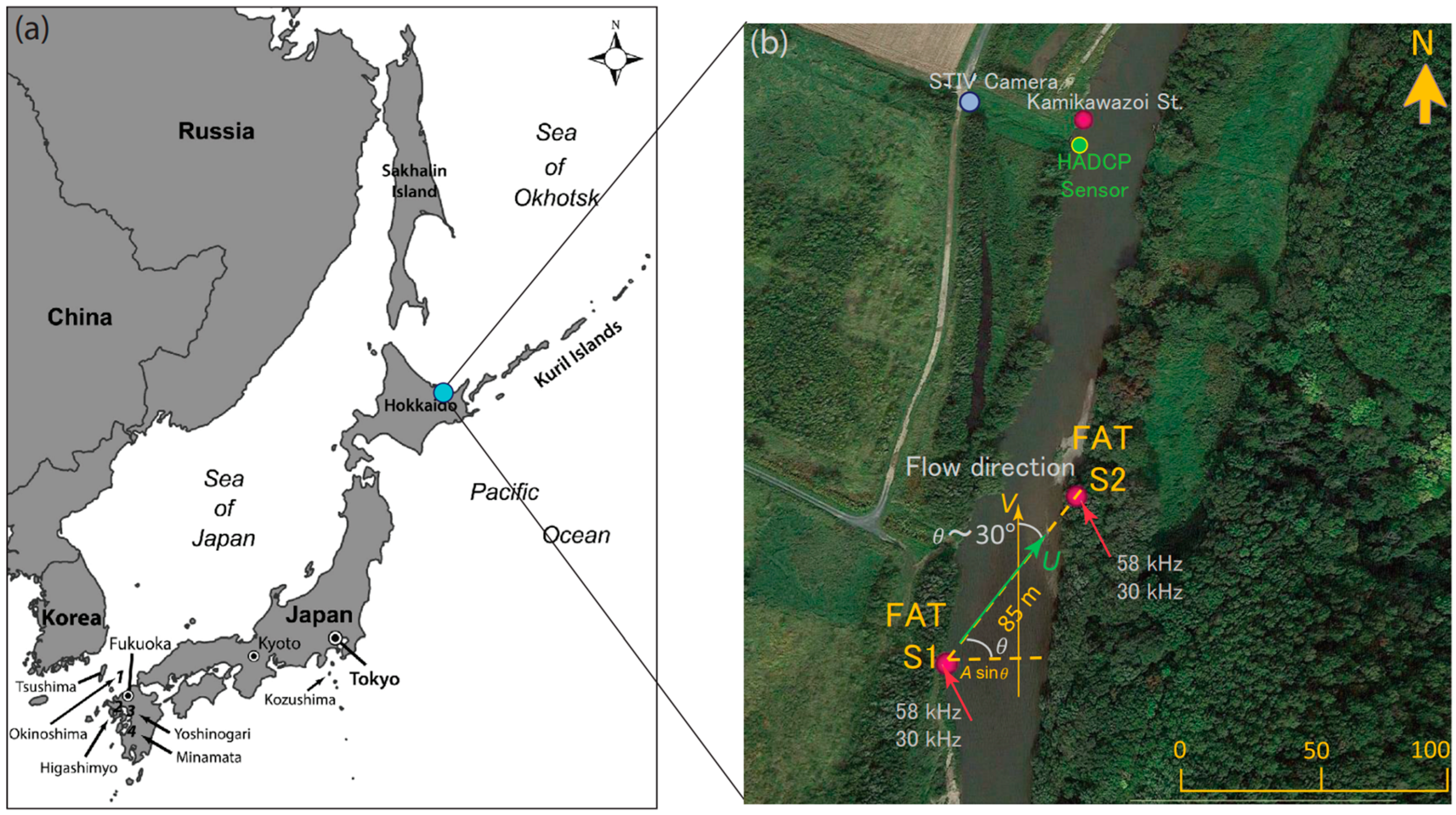
At the beginning of this research, tomographic observations by means of the FAT system were conducted using the 58 kHz system, owing to the specific features of the current monitored site. To clarify, the river channel’s mean width at the observation site was 40 m. To allow for good acoustic communication between two acoustic stations, it is recommended that the transducers should be placed in a diagonal plane, as presented in Figure 1b. Accordingly, the oblique distance was 85 m. Previous work [22] stated that the minimum distance (D_min) between a pair of transducers can be estimated using Equation (7).

$$D_{min}={\displaystyle \frac{k}{f}}\times c\times M_{sequence digits}$$

(7)

where $\kappa$ = 3 and M_{sequence digits} = 511. Moreover, the velocity resolution of the FAT system is a function of sound speed and transmission frequency and can be expressed using Equation (8).

$$V_R={\displaystyle \frac{c^2}{2\times L\times 2\times f}}$$

(8)

As can be seen in

Table 1. Information of the velocity resolution values under the minimum and current monitoring conditions.

Frequency	Minimum Conditions		Current Observation
	Dmin (m)	VR (m/s)	L (m)	VR (m/s)
58 kHz	40	0.24	85	0.11
30 kHz	76	0.24	85	0.22

, the minimum distance between a pair of 58 kHz transducers should be greater than 40 m with a velocity resolution of 0.24 m/s. Alternatively, in the case of a pair of 30 kHz transducers, the minimum distance should be greater than 76 m and the velocity resolution is 0.24 m/s. The main issue in this regard is why this observation was operated using double frequency. A comprehensive understanding of this issue necessitates examining it from two perspectives. The first perspective is the wavelength and velocity resolution, whereas the second point is the signal absorption and scattering. For the first viewpoint, it was found that the wavelength using a 58 kHz transducer estimated using Equation (6) was 2.5 cm. Alternatively, using a 30 kHz transducer, the wavelength was 5 cm. It is known that using shorter wavelengths can provide better spatial resolution, higher velocity resolution, and better accuracy, particularly in the presence of small-scale variations in water properties. Conversely, using a longer wavelength might be less sensitive to small-scale variations and results in imprecise or poorer measurements. The results presented in Table 1 showed that the velocity resolution using the 58 kHz system improved to 0.11 m/s; nonetheless, the velocity resolution using the 30 kHz system was only 0.22 m/s.

Shedding light on absorption and scattering, it is crucial to bear in mind that acoustic pulses triggered using high transmission frequency (i.e., 58 kHz) can be susceptible to absorption by suspended particles, which in turn can attenuate the signal quality and reduce the measurement precision. In simple words, the sound intensity of the acoustic pulses emitted from the 58 kHz system is weak compared to those transmitted by the 30 kHz system. Hence, there was a necessity to operate measurements using double frequency collectively. It should be noted that during past observation programs, it was possible to carry out precise measurements using the 58 kHz system only. However, the mobilization of high quantities of sediment matter in this river suggested that additional measurements using the 30 kHz system would be essential to provide complete streamflow measurements. Indeed, it was necessary to carry out either suspended sediment concentrations measurements during some flood events or at least continuous monitoring for turbidity in the site. However, this issue will be considered in future research, as permission and arrangement could not be completed in time, which in turn limited us to achieve it during this study period.

4.3. Inferences of River Flow Measurement During Very Multiple Independent Streamflow Records

It is obvious by visual inspection that the streamflow measured by the FAT system was in very good agreement with the flow records obtained by the other advanced approaches (STIV and HADCP), as depicted in case#5 and case#6 (Figure 6). Furthermore, it can be detected that the uncertainty range among these records was very low (~±20%), as demonstrated in Figure 6d. This low margin of uncertainty might be justified by the fact that these new approaches consider the temporal variations in stream velocity and the river cross-section, whereas the RC approach only considers the water stage as a function of the estimated river discharge.

Table 2. Uncertainty comparison between FAT and other reference records (RC and HADCP) using mean absolute error (MAE) and Nash–Sutcliffe efficiency (NSE) approaches.

Case No.	Streamflow Records	MAE (m3/s)	NSE
Case#5	QFAT vs. QRC	9.28	0.62
	QFAT vs. QHADCP	3.66	0.79
Case#6	QFAT vs. QRC	3.39	0.88
	QFAT vs. QHADCP	6.88	0.91

further compares the uncertainties between Q_FAT versus Q_RC, as well as Q_FAT vs. Q_HADCP, by means of the mean absolute error and Nash–Sutcliffe efficiency. It can be found that the NSE scores between FAT and HADCP records were higher in comparison to the NSE scores between FAT and RC records. Due to insufficient overlapping records between FAT and STIV records, MAE and NSE score comparisons were omitted.

An interesting question can be raised in this context. Which of the applied approaches offered accurate streamflow measures? In fact, there is no universal approach capable of providing the exact streamflow measurement in a river. Each approach has imitations; for example, measurements using an infrared camera and HADCP entail a certain water level to start streamflow measurements. Also, each measurement method has an unavoidable margin of uncertainty; this is because each river site has its own features and characteristics that form its “fingerprint”, which gives a specific measurement approach precedence over other methods. Therefore, the “true” or “exact” value of an instantaneous flow rate for a stream that passes a cross-section cannot be affirmed. Instead, the best way to maximize measurement accuracy is to increase the number of the measurement approaches utilized for a short period of time to make a better estimate.

In addition, it should be acknowledged that the key challenge of this study was the absence of a comparison between river flow records and the amount of suspended sediment mobilized during the studied flood events. Considering this issue concretely can provide us with a clear understanding of the impact of sediments on the SNR signals and the inverse relationship between the intensity of SNR signals versus the suspended sediment concentrations. The streamflow data acquired can help in improving the accuracy and reliability of river flow. One of the future plans is to continue the current monitoring program to develop multiple index velocity rating equations instead of developing a year-round RC equation.

5. Conclusions

Acquiring accurate and continuous records of streamflow data is an essential objective in river engineering design and environmental planning. With the presence of advanced river flow measurement approaches, the accuracy of river flow measurement has increased in recent years. In this research, a long-term observation program was implemented in the Tokoro River located in the Okhotsk Region of Japan. The main purpose of this research was to shed light on the extent of streamflow measurement in a very shallow and narrow silt river using the FAT system. Although the observation results were preliminary, we examined the extent of the underwater acoustic tomography system by analyzing the collected records from three different perspectives. First, an investigation under very shallow- and high-water conditions was performed. Second, an investigation by means of double acoustic frequency was carried out. Third, an investigation of acoustic measurements compared to multiple independent streamflow records was conducted. The key findings and outcomes were significant and are summarized below.

First, under extremely shallow conditions, measurement by the FAT was possible using the 58 kHz system. Encouragingly, it was found that the minimum water depth along the monitored cross-section was 9 cm, which is a new achievement in terms of monitoring capability documented so far. Furthermore, the FAT system proved its capability to measure streamflow during high water levels. Second, using double frequencies, it was found that using a high transmission frequency (i.e., 58 kHz) can provide shorter wavelengths, allowing for better spatial resolution and higher velocity resolutions and thus preferable measurement accuracy; however, measurements in the presence of high sediment particles were deficient. On the other hand, a lower transmission frequency, i.e., (30 kHz) emits a longer wavelength, which might be less sensitive to small-scale variations and leads to an imprecise degree of measurements; nevertheless, measurements can be achieved during the mobilization of high concentrations of sediments. Thirdly, using multiple streamflow measurement approaches, the findings showed that the streamflow measured by the FAT system was in very good agreement with the records obtained by the advanced measurement approaches, such as STIV and HADCP, with a very low range of uncertainty. One of the most important findings of this research was that each streamflow measurement approach has an unavoidable margin of uncertainties; this is because each river location has its own characteristics and features that configure its “fingerprint”, which gives a specific measurement approach superiority over other approaches. Therefore, the “true” or “exact” value of an instantaneous flow rate for a stream that passes a cross-section cannot be affirmed.

References

1. Kawajiri, S.; Kawaguchi, T.; Watanabe, Y.; Hayakawa, H.; Miyamori, Y.; Nakamura, D.; Yamashita, S. Investigation Report of Geotechnical Disaster on River Area Due to Typhoon Landfall Three Times on Okhotsk Region, Hokkaido, Japan. Soils Found. 2019, 59, 764–782. [Google Scholar] [CrossRef]
2. Okabe, K.; Kyuka, T.; Shimizu, Y.; Hasegawa, K.; Shinjo, K.; Yamaguchi, S. Discharge fluctuation dominating factors influencing the pass of river—A case study on otofuke river in Japan. J. Jpn. Soc. Civ. Eng. Ser. B1 (Hydraul. Eng.) 2018, 74, I_1501–I_1506. [Google Scholar] [CrossRef] [PubMed]
3. Yoshikawa, Y.; Watanabe, Y.; Hayakawa, H.; Hirai, Y. A study of ice break and ice flow during river ice breakup. J. Jpn. Soc. Civ. Eng. Ser. B1 (Hydraul. Eng.) 2011, 67, I_1075–I_1080. [Google Scholar] [CrossRef] [PubMed]
4. McMillan, H.; Seibert, J.; Petersen-Overleir, A.; Lang, M.; White, P.; Snelder, T.; Rutherford, K.; Krueger, T.; Mason, R.; Kiang, J. How Uncertainty Analysis of Streamflow Data Can Reduce Costs and Promote Robust Decisions in Water Management Applications. Water Resour. Res. 2017, 53, 5220–5228. [Google Scholar] [CrossRef]
5. Petersen-Øverleir, A. Modelling Stage-Discharge Relationships Affected by Hysteresis Using the Jones Formula and Nonlinear Regression. Hydrol. Sci. J. 2006, 51, 365–388. [Google Scholar] [CrossRef]
6. Gensen, M.R.A.; Warmink, J.J.; Berends, K.D.; Huthoff, F.; Hulscher, S.J.M.H. Improving Rating Curve Accuracy by Incorporating Water Balance Closure at River Bifurcations. J. Hydrol. 2022, 610, 127958. [Google Scholar] [CrossRef]
7. Domeneghetti, A.; Castellarin, A.; Brath, A. Assessing Rating-Curve Uncertainty and Its Effects on Hydraulic Model Calibration. Hydrol. Earth Syst. Sci. 2012, 16, 1191–1202. [Google Scholar] [CrossRef]
8. Holmes, R.R., Jr. River Rating Complexity. 2016. Available online: http://pubs.er.usgs.gov/publication/70193968 (accessed on 11 March 2025).
9. Tauro, F.; Selker, J.; van de Giesen, N.; Abrate, T.; Uijlenhoet, R.; Porfiri, M.; Manfreda, S.; Caylor, K.; Moramarco, T.; Benveniste, J.; et al. Measurements and Observations in the XXI Century (MOXXI): Innovation and Multi-Disciplinarity to Sense the Hydrological Cycle. Hydrol. Sci. J. 2018, 63, 169–196. [Google Scholar] [CrossRef]
10. Tazioli, A. Experimental Methods for River Discharge Measurements: Comparison among Tracers and Current Meter. Hydrol. Sci. J. 2011, 56, 1314–1324. [Google Scholar] [CrossRef]
11. Massó, L.; Patalano, A.; García, C.M.; Ochoa García, S.A.; Rodríguez, A. Enhancing LSPIV Accuracy in Low-Speed Flows and Heterogeneous Seeding Conditions Using Image Gradient. Flow Meas. Instrum. 2024, 100, 102706. [Google Scholar] [CrossRef]
12. Fujita, I.; Notoya, Y.; Tani, K.; Tateguchi, S. Efficient and Accurate Estimation of Water Surface Velocity in STIV. Environ. Fluid Mech. 2019, 19, 1363–1378. [Google Scholar] [CrossRef]
13. Tsubaki, R. On the Texture Angle Detection Used in Space-Time Image Velocimetry (STIV). Water Resour. Res. 2017, 53, 10908–10914. [Google Scholar] [CrossRef]
14. Sutarto, T.E. Application of Large Scale Particle Image Velocimetry (LSPIV) to Identify Flow Pattern in a Channel. Procedia Eng. 2015, 125, 213–219. [Google Scholar] [CrossRef]
15. Armstrong, D.W.; Holnbeck, S.R.; Chase, K.J. Evaluating the Use of Video Cameras to Estimate Bridge Scour Potential at Four Bridges in Southwestern Montana. 2022. Available online: https://pubs.usgs.gov/publication/fs20223040 (accessed on 11 March 2025).
16. Al Sawaf, M.B.; Kawanisi, K.; Xiao, C. Measuring Low Flowrates of a Shallow Mountainous River Within Restricted Site Conditions and the Characteristics of Acoustic Arrival Times Within Low Flows. Water Resour. Manag. 2020, 34, 3059–3078. [Google Scholar] [CrossRef]
17. Nihei, Y.; Kimizu, A. A New Monitoring System for River Discharge with Horizontal Acoustic Doppler Current Profiler Measurements and River Flow Simulation. Water Resour. Res. 2008, 44, 6970. [Google Scholar] [CrossRef]
18. Kawanisi, K.; Razaz, M.; Ishikawa, K.; Yano, J.; Soltaniasl, M. Continuous Measurements of Flow Rate in a Shallow Gravel-Bed River by a New Acoustic System. Water Resour. Res. 2012, 48, 1–10. [Google Scholar] [CrossRef]
19. Al Sawaf, M.B.; Kawanisi, K.; Gusti, G.N.N.; Khadami, F.; Xiao, C.; Bahreinimotlagh, M. Continuous Measurement of Flow Direction and Streamflow Based on Travel Time Principles Using a Triangular Distribution of Acoustic Tomography Systems. J. Hydrol. 2023, 617, 128917. [Google Scholar] [CrossRef]
20. Xiao, C.; Kawanisi, K.; Al Sawaf, M.B.; Zhu, X.H. Assessment of Flood Dynamics in a Mountain Stream Using High-resolution River Flow Records. Hydrol. Process. 2023, 37, 14841. [Google Scholar] [CrossRef]
21. Falvey, H.T. Effect of Gradients on Acoustic Velocity Meter. J. Hydraul. Eng. 1983, 109, 1441–1453. [Google Scholar] [CrossRef]
22. Bahreinimotlagh, M.; Kawanisi, K.; Danial, M.M.; Al Sawaf, M.B.; Kagami, J. Application of Shallow-Water Acoustic Tomography to Measure Flow Direction and River Discharge. Flow Meas. Instrum. 2016, 51, 30–39. [Google Scholar] [CrossRef]
Figure 1. (a) Position of the study region in Japan and (b) aerial image of the observation area and location of measurement instruments.
Water 17 00831 g001
Figure 2. (a) FAT monitoring unit installed at the right bank, (b) FAT system logger and battery, (c) deployment of the underwater transducers at the right bank in shallow-flow conditions, and (d) detailed representation of the transducer deployment.
Water 17 00831 g002
Figure 3. Temporal variations in the water level as measured at Kamikawazoi Station in (a) 2023 and (b) 2024.
Water 17 00831 g003
Figure 4. Time-series of (a) water level at Kamikawazoi St., (b) streamwise cross-sectional velocity measured by FAT 58 kHz, (c) streamflow measurements using QFAT 58 kHz (black) and QRC (red), (d) uncertainty between QFAT 58 kHz vs. QRC (black), and (e) performance of FAT SNR signals during the studied events.
Water 17 00831 g004
Figure 5. Time-series of (a) water level at Kamikawazoi St., (b) streamwise cross-sectional velocity measured by FAT 58 kHz (black) and FAT 30 kHz (blue), (c) streamflow measurements using QFAT 58 kHz (black), QFAT 30 kHz (blue), and QRC (red), (d) uncertainty between QFAT 58 kHz vs. QRC (black) and between QFAT 30 kHz vs. QRC (blue), and (e) performance of FAT SNR signals during the studied events.
Water 17 00831 g005
Figure 6. Time-series of (a) water level at Kamikawazoi St., (b) streamwise cross-sectional velocity measured by FAT 58 kHz (black), (c) streamflow measurements using QFAT 58 kHz (black), QRC (red), QHADCP (green), and QSTIV (brown), (d) uncertainty between QFAT 58 kHz vs. QRC (red), uncertainty between QFAT 58 kHz vs. QHADCP (green), uncertainty between QFAT 58 kHz vs. QSTIV (black), and (e) performance of FAT SNR signals during the studied events.
Water 17 00831 g006
Figure 7. Illustration for the cross-sectional area shape along the transmission line when the water level at Kamikawazoi Station is 2.2 m.
Water 17 00831 g007
Figure 8. Demonstration of the high-turbid state of the monitoring site during extremely shallow conditions caused by a very gentle rainfall event.
Water 17 00831 g008