Assessment of Low-Flow Trends in Four Rivers of Chile: A Statistical Approach

Abstract

Understanding and analyzing low river flows are some of key tasks of effective water management, particularly in Chile’s Mediterranean regions, where irregular rainfall distribution leads to drought and water scarcity. This study aims to assess low-flow trends in the four major Chilean river basins (Maipo, Rapel, Maule, and Biobío) by calculating three key hydrological indices: the mean annual minimum and maximum flows (MAM), the base flow index (BFI), and the standardized precipitation index (SPI), using data from 18 hydrometric stations. The indicators of hydrologic alteration (IHA) tool was applied to calculate the MAM and BFI to assess flow variability and groundwater contributions. The SPI was calculated to examine hydrological drought conditions and evaluate how these conditions affect river flow behavior, correlating reduced low river flows with precipitation trends at the beginning of the dry season. Statistical analysis was conducted through the ordinary least squares (OLS) test for normally distributed data, and non-parametric tests, including the Mann–Kendall test, as well as Sen’s slope estimation, for data not meeting normality requirements. The results, presented both analytically and graphically, reveal trends in river flow indices and variations across the river basins, identifying critical areas of reduced flow that may require enhanced water management strategies.

1. Introduction

Global warming, changes in precipitation patterns, loss and reduction of cryospheric elements, and increased frequency and intensity of climatic extremes are some of water-related climate change effects [1]. Additionally, about half of the global population currently faces severe water scarcity for at least a part of the year, due to climatic and non-climatic variables [1]. The latter are related to demands from rapidly growing populations and global economies for domestic, industrial, and agricultural uses [2].

Internationally, it has been proposed that the current water crisis not only comprises water scarcity in the physical and ecological dimensions, but also, it is related to ineffective water resources management [3]. This may involve, among other factors, the absence of sufficient information, which is often scarce, fragmented, and outdated [4]. In this sense, it is very important to understand where, how many, and how variable water resources are (today and in future scenarios) to achieve better water management and governance [5]. The academic and policy communities have acknowledged the importance of counting on reliable, accurate, and up-to-date information for decision-making grounded in evidence [2]. Therefore, it is necessary to have tools to make informed decisions based on data.

Watercourse variability significantly impacts the quality and quantity of the water available for both social and ecological purposes. However, human activities have altered the natural flow patterns of most river systems [6]. Therefore, in river basins with intense human activity, it is crucial to have a comprehensive understanding of how seasonal and annual minimum flows vary in inland waters—both upstream and downstream—to ensure effective water resource management.

Different paradigms and initiatives related to water management and governance have referred to the significance of data to achieve efficient decision making. For instance, The Organization for Economic Co-operation and Development (OECD)’s water governance framework [7], the Principle 5, promotes the creation of coordinated basin-scale information systems to provide timely, reliable, and comparable water-related data. These data should support the development, evaluation, and improvement of water policies. In addition, the integrated water resources management paradigm (IWRM) claims the need for a water resources knowledge base (concerning hydrological cycle and associated ecosystems) as a management instrument that assesses the resource and defines its natural limits for effective management implementation [4].

In Mediterranean-climate regions, rivers act especially as a primary source of water. They are characterized by highly variable precipitation patterns, an extended dry season, and an insufficient quantity of natural lakes, unlike humid regions where consistent rainfall throughout the year irrigates crops and refills reservoirs [8]. Particularly in Mediterranean-climate regions, climate change increases risk and uncertainty by intensifying hydrological variability as the climate variability increases [9].

The central zone of Chile is one of the Mediterranean-climate regions existing in the world, which is located between the Aconcagua and Biobío River basins (32–40° S) [10]. Topographically, this region is characterized by the presence of two parallel mountain ranges from north to south: the Coastal Cordillera and the Andes Mountain range, separated by a narrow Central valley (80–100 km wide) [11]. The latter influence precipitation patterns across the country, affecting both temperature and precipitation [12]. Additionally, El Niño (ENSO), Pacific Decadal (PDO), and the Antarctic (AAO) oscillations influence the Chilean climate. During years dominated by ENSO, precipitation is more likely, and in combination with PDO, it significantly influences snow accumulation and mountain flow patterns [12].

The central valley of Chile, the warmest area, is 5–6 °C hotter than coastal areas due to the coastal mountains acting as a barrier to maritime influence [10]. Winter frosts occur in the Andes mountains, and precipitation, concentrated from May to July (300–1500 mm/year) [13], increases river flows and leads to ice and snow accumulation above 1500 m.a.s.l. [14]. The melting of this snow and ice sustains permanent river flows throughout austral summer. However, for this area of the world, climate change predictions estimate a general decrease in precipitation (up to 30% in relation to current values) and an up to 4 °C increase in temperature [15].

While climate change will intensify the hydrological impacts on fluvial systems, the primary cause of reduced flows at present is the high rate of water extractions, posing a significant challenge for water governance [16]. A country’s vulnerability to the water crisis is influenced not only by its climate but also by how its water resources are managed, and Chile is no exception to this reality [17]. Chile has a distinctive governance system based on water use privatization and market-based instruments to reallocate water resources, which has led to the promotion of agricultural, hydroelectric, and mining investments located in the country’s main river basins.

In a country where rainfall is so highly variable and where water resources are used intensively, information on the availability of these resources and their effective management is vital to ensure economic, social, and environmental sustainability. In this sense, the purpose of this study is to identify and analyze low-flow trends in four Chilean rivers and their relationship with water use and water management features. Trend analysis aims to determine how the statistical characteristics of hydrological variables could change over time at various sites within a basin. Understanding these trends is essential for assessing regional hydrological stability and supporting water management strategies in the face of climate variability.

2. Materials and Methods

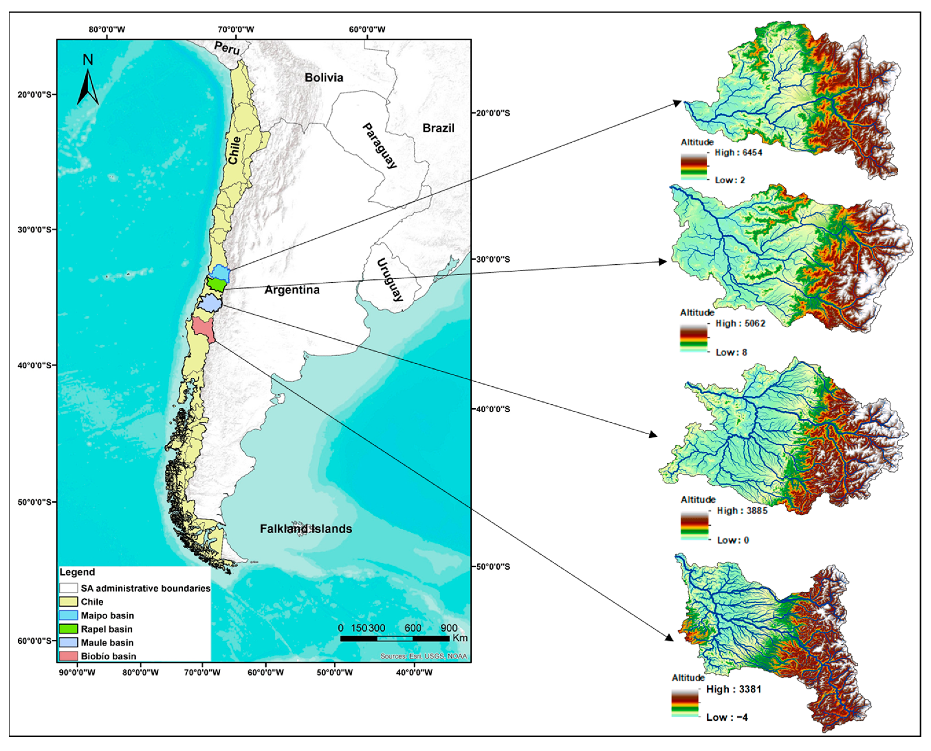
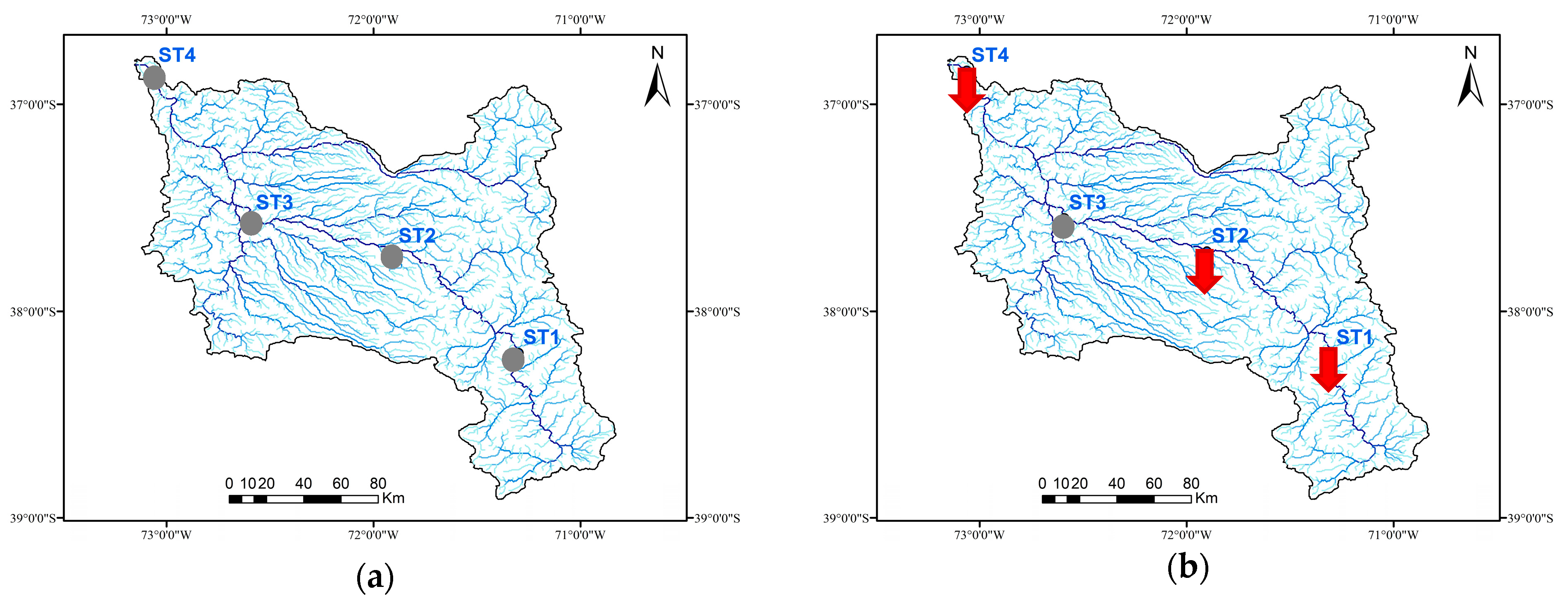
2.1. Study Area

In Chile, large rivers flow from the Andes Mountain range to the Pacific Ocean, following high topographic gradients and being influenced by different climatic, geographical and geological configurations [18]. For the sake of this study, four river basins were selected (Figure 1), whose main characteristics are listed in

Table 1. Main characteristics of the study area.

	Maipo	Rapel	Maule	Biobío
Basin area (km2)	15,273 [19]	13,766 [19]	21,052 [19]	24,369 [19]
Location	32°55′ and 34°15′ south latitude	33°53′ and 35°01′ south latitude	35°05′ and 36°30′ south latitude	36.7° and 38.9° south latitude
River length (Km)	225 [19]	240 [10]	213 [19]	370 [19]
Climate	Mediterranean semi-arid [20]	Mediterranean template [21]	Temperate Mediterranean [22]	Wet–temperate with a Mediterranean influence [23]
Average discharge (m3 s−1)	145,.67 m3/s [24]	Cachapoal: 89.0 m3/s Tinguiririca: 50.2 m3/s [19]	467 m3/s [25]	1000 m3/s [26]
Mean annual precipitation	380 mm [27]	898 mm [28]	735 mm [29]	1746.72 mm [30]
Sub-basins	Maipo Alto, Maipo Medio, Mapocho Alto, Mapocho Bajo, and Maipo Bajo [31]	Cachapoal alto, Cachapoal bajo Tinguiririca alto, Tinguiririca bajo, Alhue, and Rapel [31]	Maule Alto, Melado, Maule Medio, Perquilauquen Alto, Perquilauquen Bajo, Loncomilla, Maule entre Loncomilla y Claro, Claro, Maule Bajo [31]	Río Biobío Alto (hasta después junta Río Lamin), Río Biobío entre Río Ranquil y Río Duqueco, Río Duqueco, Río Biobío entre Río Duqueco y Río Vergara, Río Renaico, Ríos Malleco y Vergara, Río Biobío entre Río Vergara y Río Laja, Río Laja Alto (hasta bajo junta Río Rucue), Laja Bajo, Río Biobío Bajo [31]
Population	7,112,808 96.3% urban [32]	866,000 72% urban [32]	852,035 72.1% urban 38.9 rural [33]	1,400,000 90% urban [32]
Agriculture water demands	61.6% of total water use [34]	93% of total water use [35]	26% of total water use [36]	42% of total water use [34]
Drinking water demands	659,893 Mm3/year urban 11,570 Mm3/year rural [34]	43,074 Mm3/year urban 28,524 Mm3/year rural [34]	31,240 Mm3/year urban 11,240 Mm3/year rural [33]	41,745 Mm3/year Urban 4575 Mm3/year Rural [34]
Industry water demands	38,468 Mm3/year [34]	12,276 Mm3/year [34]	35,500 Mm3/year [33]	350,470 Mm3/year [34]
Mining water demands	23,442 Mm3/year [34]	70,721 [34]	-	-
Energy water demands	300 MW [20]	26 hydroelectric power plants 1033.85 MW [28]	25 hydroelectric power plants 447.01 m3/s 1680 MW [33]	17 hydroelectric power plants, producing more than 2800 MW) [37] 17% of total water consumption [34]

.

2.2. Data Collection

The methodology adopted in this study consists of the collection of hydrological data focusing on river flows, their preprocessing, and statistical analysis, including trend detection and correlation with drought indices, to evaluate flow characteristics over time.

Hydrological analysis is highly dependent upon data quality and availability. For this study, daily river flow data from 18 hydrometric stations (

Table 2. Hydrometric stations of the river basins.

Basin	Stations		Latitude	Longitude	Altitude (m)
Maipo River	ST1	Río Maipo en las Hualtatas	33°59′	70°10′	1820
	ST2	Río Volcan en Queltehues	33°48′	70°12′	1365
	ST3	Río Colorado antes junta Río Olivares	33°30′	70°08′	1500
	ST4	Río Olivares antes junta Río Colorado	33°29′	70°08′	1500
	ST5	Río Colorado antes junta Río Maipo	33°59′	70°22′	890
	ST6	Río Maipo en El Manzano	33°35′	70°24′	850
Rapel River	ST1	Río Cachapoal en Puente Termas de Cauquenes	34°15′00″	70°34′00″	700
	ST2	Estero La Cadena antes junta Río Cachapoal	34°11′03″	70°50′37″	440
	ST3	Río Tinguiririca Bajo los Briones	34°43′07″	70°49′36″	560
	ST4	Río Tinguiririca en los Olmos	34°29′32″	71°22′23″	223
Maule River	ST1	Canal Maule Sur en Aforador	35°38′20″	71°23′02″	315
	ST2	Canal Duao Zapata	35°35′21″	71°32′09″	0
	ST3	Río Maule en Longitudal	35°33′27″	71°42′24″	90
	ST4	Río Maule en Forel	35°24′25″	72°12′30″	30
Biobío River	ST1	Río Biobío en Llanquén	38°12′03″	71°17′56″	767
	ST2	Río Biobío en Rucalhue	37°42′38″	71°54′06″	261
	ST3	Río Biobío en Coihue	37°33′01″	72°35′25″	60
	ST4	Río Biobío en Desembocadura	36°50′19″	73°03′43″	16

) across all four Mediterranean basins in Chile were used, over the period from 1980 to 2016, creating a flow time series of approximately 37 operating years per station. The data were obtained from the General Water Directorate (DGA), Chile, which is responsible for the management and distribution of water use rights, and reports to the Ministry of Public Works.

2.3. Data Pre-Processing

Before analysis, the datasets were checked for completeness and potential inconsistencies, such as outliers or gaps in the time series. Hydrologic yearbooks and specific-gauge analysis were used to identify any data discontinuities or database errors [38]. These were corrected when possible or else removed from subsequent analysis. After the cleaning process, the data were formatted for hydrological and statistical analysis.

The conversion of the acquired data into a continuous time series required the use of computational tools for their systematic formatting. More specifically, a programming tool was used to consolidate the time series for each region and format them according to a template that would allow further statistical processing. This tool also removes the outliers and calculates the percentage of blank values for each station, helping in the formatting process. Outliers were removed by visual inspection while plotting the data using scatter plots and comparing the outliers’ values with historical flow records representing extreme meteorological and hydrological conditions (e.g., extreme rainfall events).

As with most time series of flow data, this particular time series had a number of blank values scattered throughout the time series. Since the calculation of the low-flow indicators requires a complete time series with data without blank values, an additional tool has been created to fill in the blanks following international standards. In this particular case, an attempt was first made to fill in the blank values using the linear interpolation method. However, as this was a low-flow study, this method appeared to affect the subsequent calculation of the indicators and was, therefore, eventually replaced by filling in the blanks with average values. The “mean filling” means filling in the blanks with the average of the last available recorded flow before the blank and the first available recorded value after the blank.

Coordinates, basin area size, and other descriptive elements of each station were organized to allow for mapping and categorization of the stations according to their location in the catchment area (upstream/downstream).

2.4. Statistical Analysis

The IHA tool [39,40] was applied to calculate flow indices, such as the mean annual minimum and mean annual maximum flows (1, 7, 30, and 90 days), and BFI for each station during the study period. Developed by The Nature Conservancy, the IHA tool assesses changes in hydrological flow regimes by computing flow statistics, such as flow magnitude, frequency, and duration [39]. This tool is particularly suited for analyzing natural or anthropogenic influences on hydrologic patterns, and its non-parametric approach is effective for datasets that may not be normally distributed [41]. These indicators were chosen because they provide an overview of low-flow behavior on different time scales [42,43].

The flow time series data were tested for normality, using the Kolmogorov–Smirnov test [44] (significance level of α ≤ 5%) to detect trends and correlations. Time series failing the normality test were reserved for non-parametric trend analysis, while normally distributed data were subjected to parametric analysis.

For the indices that followed a normal distribution, ordinary least squares (OLS) regression was used to detect trends and calculate slope. For non-normally distributed data, the Mann–Kendall (MK) test [45], a non-parametric method, was applied to detect trends, with Sen’s slope estimator used to quantify the magnitude of the trend detected.

The SPI, a widely used drought index, was calculated to assess long-term precipitation patterns. Frequently applied in hydrological studies, the SPI serves as a probabilistic measure of precipitation variability across multiple time scales, enabling effective analysis of both short-term and long-term wet and dry conditions [46]. SPI values were derived by using the rainfall data from selected stations within the basin, and the results were correlated with March flow values, marking the ending of the dry season in the Southern Hemisphere and the 7-day minimum flow. This correlation helped explore how drought conditions, as indicated by SPI values, influenced river low flow over the study period.

The analysis results were consolidated in tables and time series plots showing low-flow indices over the study period. Spatial distribution maps were created to visualize trend variations across different stations, helping to identify areas with significant flow declines or increases over time. This comprehensive approach aligns with the study’s aim of assessing low-flow trends in the study area and identifying areas of potential concern for water management.

3. Results

3.1. Flow Trends and Statistical Analysis

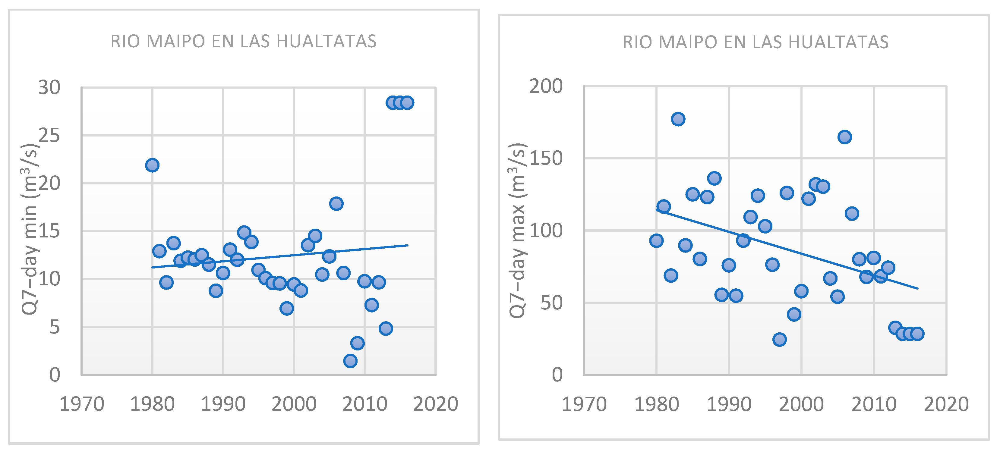
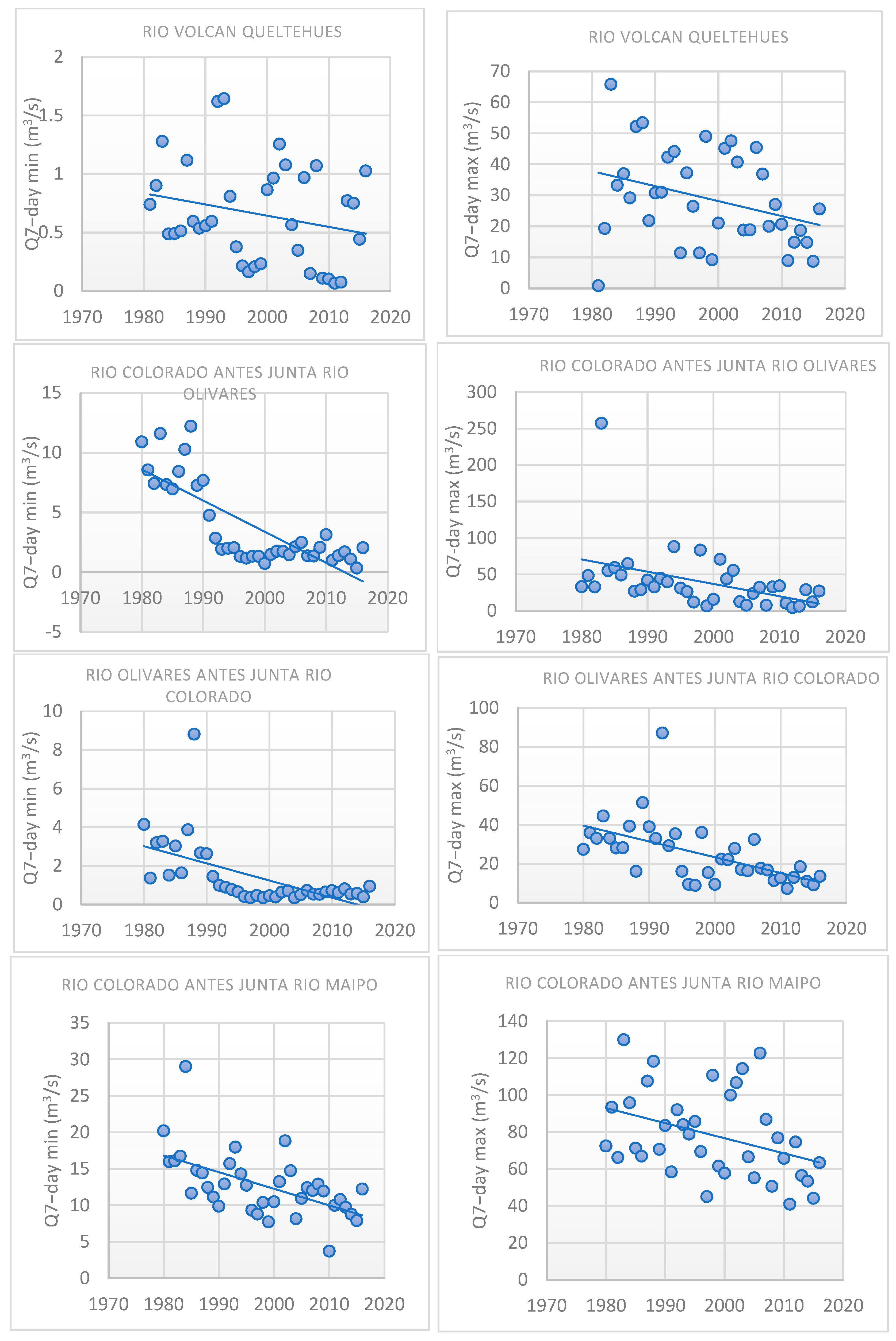
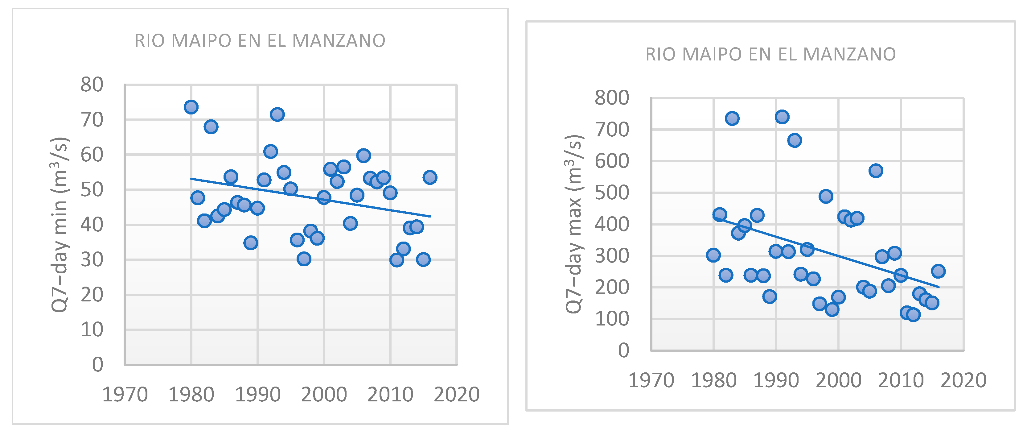
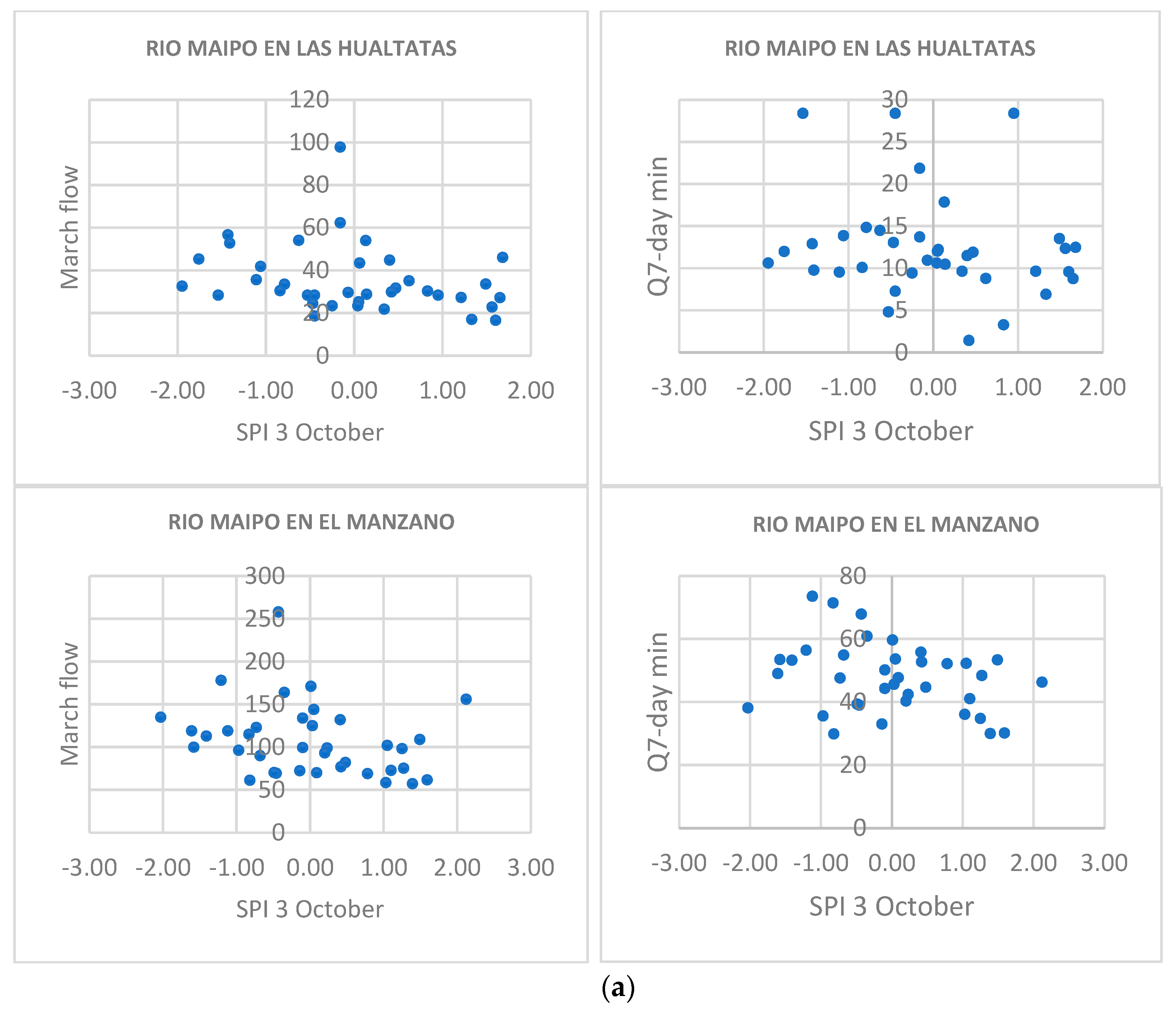
3.1.1. Maipo River Basin

The table below (

Table 3. Trends and normality tests of low and high-flow time series for the Maipo River.

Station Name	Río Maipo En Las Hualtatas				Station Name	Río Volcan En Queltehues
Indices (m3/s)	Norm test Result	Flow Range (m3/s)	Slope	p-Value	Indices (m3/s)	Norm test Result	Flow Range (m3/s)	Slope	p-Value
1-day min	normal	1.15–28.4	0.150	0.250	1-day min	normal	0.0530–1.46	−0.003	0.50
3-day min	normal	1.37–28.4	0.128	0.250	3-day min	normal	0.0563–1.48	−0.003	0.50
7-day min	normal	1.44–28.4	0.124	0.250	7-day min	normal	0.0676–1.64	−0.002	0.50
30-day min	normal	1.61–28.4	0.110	0.250	30-day min	normal	0.1251–2.4	−0.002	0.50
90-day min	normal	6.60–30.1	0.106	0.250	90-day min	normal	0.3244–4.76	−0.005	0.50
1-day max	normal	27.00–181	−1.740	0.005	1-day max	normal	0.9570–71.5	−0.508	0.10
3-day max	normal	26.07–180	−1.700	0.005	3-day max	normal	0.9110–69.7	−0.473	0.10
7-day max	normal	24.39–177	−1.630	0.005	7-day max	normal	0.8544–65.9	−0.395	0.10
30-day max	normal	23.43–165	−1.440	0.005	30-day max	normal	0.7787–58.6	−0.323	0.25
90-day max	normal	20.77–139	−1.220	0.005	90-day max	normal	0.7662–49.5	−0.288	0.10
Station Name	Río Colorado Antes Junta Río Olivares				Station Name	Río Olivares Antes Junta Río Colorado
Indices (m3/s)	Norm test Result	Flow Range m3/s	Slope	p-Value	Indices (m3/s)	Norm test Result	Flow Range m3/s	Slope	p-Value
1-day min	not	0.369–14.8	−0.24	0.001	1-day min	not	0.284–7.92	−0.074	0.001
3-day min	not	0.369–14.8	−0.25	0.001	3-day min	not	0.339–8.18	−0.076	0.001
7-day min	not	0.369–14.8	−0.26	0.001	7-day min	not	0.346–8.82	−0.082	0.001
30-day min	not	0.369–14.8	−0.28	0.001	30-day min	not	0.385–10.9	−0.098	0.001
90-day min	not	0.664–18.4	−0.31	0.001	90-day min	not	0.423–13.1	−0.121	0.001
1-day max	normal	6.59–262	−1.74	0.005	1-day max	normal	8.710–91.9	−0.809	0.001
3-day max	normal	4.903–192	−1.48	0.005	3-day max	normal	8.543–90.2	−0.821	0.001
7-day max	normal	4.674–182	−1.4	0.005	7-day max	normal	7.220–87	−0.84	0.001
30-day max	normal	3.828–149	−1.15	0.005	30-day max	normal	3.690–71.8	−0.817	0.001
90-day max	normal	3.156–142	−1.05	0.005	90-day max	normal	2.173–35.6	−0.715	0.001
Station Name	Río Colorado Antes Junta Río Maipo				Station Name	Río Maipo En El Manzano
Indices (m3/s)	Norm test Result	Flow Range m3/s	Slope	p-Value	Indices (m3/s)	Norm test Result	Flow Range m3/s	Slope	p-Value
1-day min	normal	2.13–19.8	−0.14	0.005	1-day min	normal	26.40–70.8	−0.111	0.500
3-day min	normal	2.17–25.6	−0.18	0.005	3-day min	normal	27.37–72.1	−0.127	0.500
7-day min	normal	3.71–29	−0.19	0.005	7-day min	normal	29.90–73.6	−0.146	0.500
30-day min	normal	8.13–33.2	−0.20	0.005	30-day min	normal	32.03–85.8	−0.184	0.500
90-day min	normal	8.55–50.9	−0.26	0.025	90-day min	normal	33.43–91.2	−0.188	0.500
1-day max	normal	44.30–135	−1.32	0.001	1-day max	normal	135.0–1135	−6.951	0.025
3-day max	normal	42.90–133	−1.02	0.005	3-day max	normal	120.7–985	−6.5	0.025
7-day max	normal	40.89–130	−0.93	0.01	7-day max	normal	113.0–740	−6.265	0.010
30-day max	normal	34.24–119	−0.9	0.005	30-day max	normal	100.4–654	−4.761	0.010
90-day max	normal	28.14–105	−0.97	0.001	90-day max	normal	87.06–533	−3.592	0.010

) presents the hydrological trends observed for the Maipo River across the six stations, with low-flow and high-flow indicators (1-day to 90-day minimum and maximum) analyzed. Statistically significant decreases in low-flow rates, as well as high-flow rates, were observed at most stations, highlighting significant alterations.

The low-flow indices showed variability in their normal distribution. Stations such as Río Colorado antes junta Río Maipo, Río Maipo en El Manzano, Río Maipo en Las Hualtatas, and Río Volcan en Queltehues followed a normal distribution. In contrast, the flow records of the Río Colorado antes junta Río Olivares and Río Olivares antes junta Río Colorado stations were not normally distributed. On the other hand, high-flow rates followed a normal distribution across all stations.

For example, low-flow trends, such as the 90-day minimum at Río Colorado antes junta Río Olivares, showed a considerable negative slope of −0.310 and a highly significant p-value of 0.001. Similarly, Río Olivares antes junta Río Colorado, all low flows, showed a statistically significant decline, such as a 7-day minimum flow with a slope of −0.082 and p-value of 0.001. Some indicators remain stable, such as the 1-day minimum flow in Río Maipo en El Manzano, which shows no significant change (p-value of 0.5).

For high-flow trends, such as, for example, at Río Colorado antes junta Río Maipo, the 1-day maximum flow decreased, with a slope value of −1.320 and a p-value of 0.001. At Río Maipo en El Manzano, the 1-day maximum flow showed a steep decrease, with a slope of −6.951 and a p-value of 0.025.

The plots (Figure 2) visually confirm the significant decreases in low flows at most stations, except for Río Maipo en Las Hualtatas, which shows a slight increase that is not significant. High flows show significant decreases in high flows across all stations, as highlighted in the tables.

The spatial distribution of these trends is visualized in the maps (Figure 3), confirming the significant decreases in low flows at most upstream stations. High flows also show decreasing trends across all stations.

3.1.2. Rapel River Basin

For the Rapel River, hydrological trends were analyzed across four stations (

Table 4. Trends and normality tests of low and high-flow time series for the Rapel River.

Station Name	Cachapoal En Puente Termas De Cauquenes				Station Name	Estero La Cadena Antes Junta Río Cachapoal
Indices (m3/s)	Norm Test Result	Flow Range m3/s	Slope	p-Value	Indices (m3/s)	Norm Test Result	Flow Range m3/s	Slope	p-Value
1-day min	normal	0.225–2.590	0.041	0.500	1-day min	normal	0.225–5.54	−0.004	0.500
3-day min	normal	0.239–2.667	0.044	0.500	3-day min	normal	0.2727–6.16	−0.005	0.500
7-day min	normal	0.281–3.166	0.056	0.500	7-day min	normal	0.3246–6.461	−0.006	0.500
30-day min	normal	0.426–4.418	0.086	0.250	30-day min	normal	0.4808–8.575	−0.006	0.500
90-day min	normal	1.130–7.130	−0.049	0.500	90-day min	normal	1.108–11.38	−0.028	0.500
1-day max	normal	62.30–618.0	−37.95	0.001	1-day max	normal	10.3–239	−3.052	0.005
3-day max	normal	53.53–540.0	−31.07	0.001	3-day max	normal	9.557–168	−2.295	0.010
7-day max	normal	44.57–515.9	−24.41	0.010	7-day max	normal	8.736–132.8	−1.552	0.010
30-day max	normal	26.81–461.1	−19.37	0.025	30-day max	normal	7.692–64.81	−0.761	0.010
90-day max	normal	21.58–330.3	−13.76	0.025	90-day max	normal	5.025–53.32	−0.386	0.025
Station Name	Río Tinguirririca Bajo Los Briones				Station Name	Río Tinguirririca En Los Olmos
Indices (m3/s)	Norm Test Result	Flow Range m3/s	Slope	p-Value	Indices (m3/s)	Norm Test Result	Flow Range m3/s	Slope	p-Value
1-day min	not	2.23–94.21	−0.499	0.10	1-day min	normal	0.245–11.20	−0.427	0.050
3-day min	not	3.85–94.28	−0.458	0.10	3-day min	normal	0.279–11.40	−0.432	0.050
7-day min	not	5.23–94.42	−0.454	0.10	7-day min	normal	0.299–11.50	−0.561	0.025
30-day min	not	6.18–95.23	−0.524	0.05	30-day min	normal	0.571–20.15	−0.515	0.500
90-day min	not	8.84–97.33	−0.566	0.05	90-day min	normal	0.744–38.27	−0.867	0.500
1-day max	normal	61.60–521.0	1.920	0.50	1-day max	normal	162.0–1554.0	−28.62	0.500
3-day max	normal	58.73–506.6	0.810	0.50	3-day max	normal	157.7–887.3	−11.14	0.500
7-day max	normal	57.24–499.4	0.510	0.50	7-day max	normal	135.6–491.9	−4.824	0.500
30-day max	not	47.50–457.9	0.414	0.50	30-day max	normal	75.51–297.1	−4.138	0.500
90-day max	normal	45.20–351.0	0.161	0.50	90-day max	normal	51.16–227.1	−5.468	0.050

).

The station Cachapoal en Puente Termas de Cauquenes displayed an increase in the low-flow indices, as indicated by a positive slope, with no statistical significance (e.g., 1-day minimum flow slope of 0.041 with a p-value of 0.5). An exception was observed for the 90-day minimum flow, which exhibited a tendency to decrease. In contrast, high-flow rates showed declining trends across all the timescales (e.g., 1-day maximum flow slope of −37.95 and p-value of 0.001). All examined indicators follow the normal distribution.

For the station Estero La Cadena antes junta Río Cachapoal, there are slight decreases in the low-flow indices, without statistical significance, such as the 90-day minimum (slope of −0.028 and p-value of 0.5). The high-flow indices showed more pronounced and statistically significant declines (e.g., 1-day maximum flow slope of −3.052 and p-value of 0.005). All examined indicators follow a normal distribution.

For the station Río Tinguiririca Bajo Los Briones, there are trends that show a decrease in the low-flow indices, such as the 30-day minimum flow slope of −0.524 and a p-value of 0.05). In contrast, high-flow indices showed an increasing tendency (e.g., 30-day maximum flow with a positive slope of 0.41 and p-value of 0.5). Low-flow indices did not follow a normal distribution, whereas the high-flow indices did.

For the Río Tinguiririca en Los Olmos, low-flow indices exhibited declining trends, particularly during short-duration events, with the 7-day minimum flow (slope of −0.566 and p-value of 0.025) showing a significant reduction. High-flow indices showed a decrease with no significance (e.g., 1-day maximum flow had a negative slope of −28.62 and a p-value of 0.5). All examined indicators followed a normal distribution.

The 7-day minimum and maximum flow plots for the Rapel River (Figure 4) stations represent the trends observed in Table 4. These plots visually confirm a non-significant increase in the low flows at the Cachapoal en Puente Termas de Cauquenes station, as well as non-significant decreases at other stations, except the downstream station, which exhibits a significant decrease. High flows show a more significant decrease at the upstream stations and remain stable downstream.

In addition, these trends are visualized in the spatial distribution of low- and high-flow trends, confirming the observed analysis (Figure 5). The downstream station shows a significant decrease, while the upstream stations show non-significant trends. And high flows are more pronounced at the upstream stations.

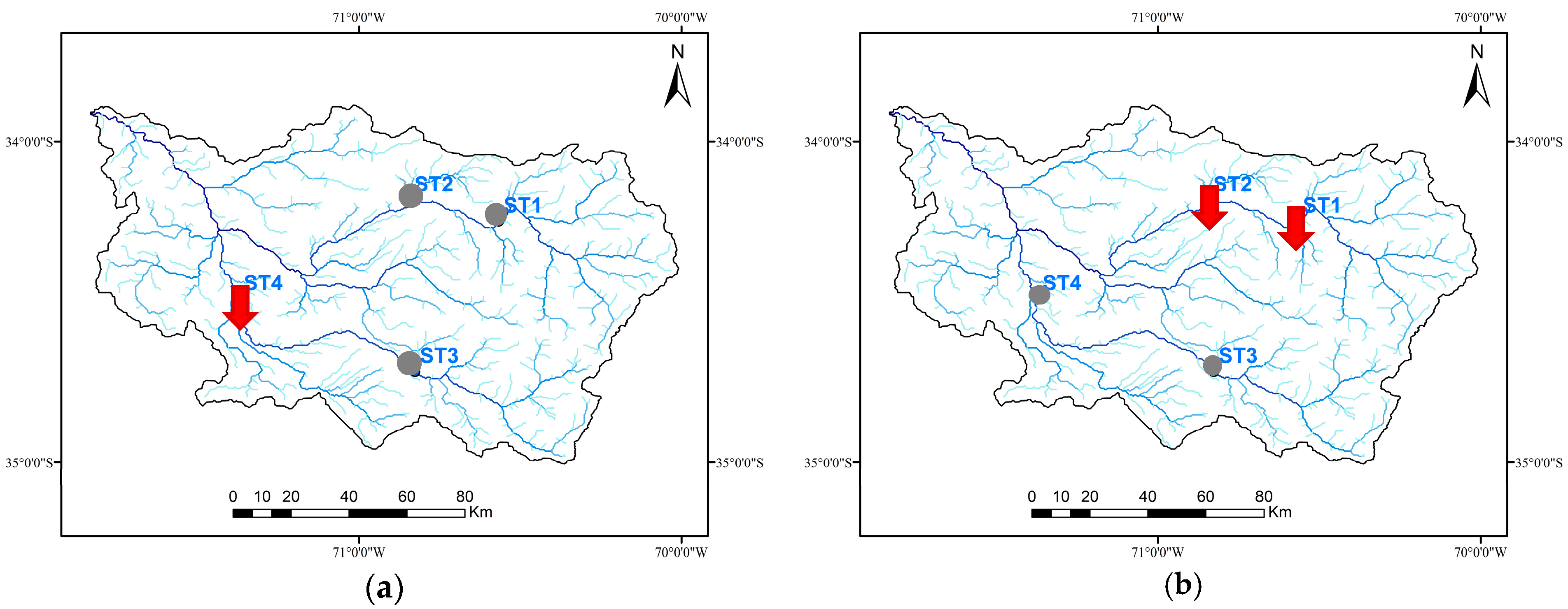
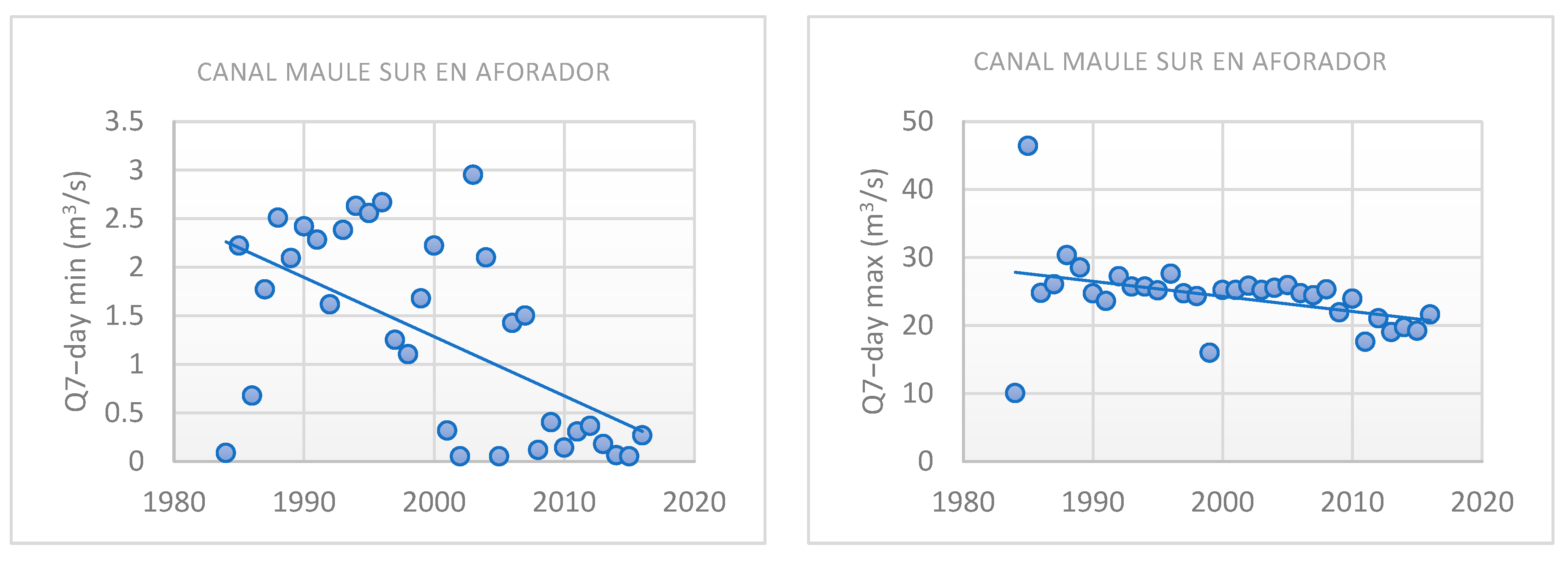
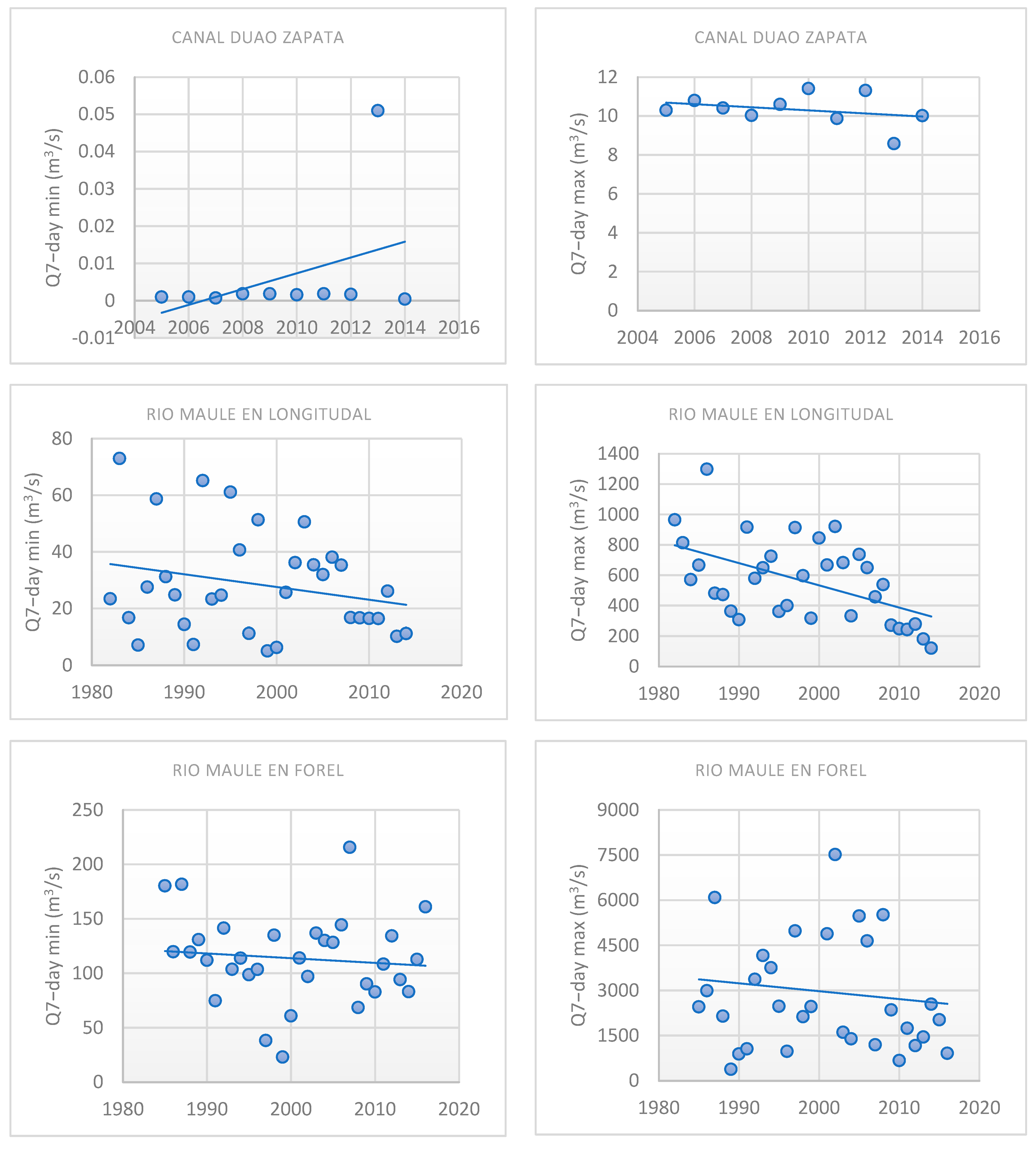
3.1.3. Maule River Basin

For the Maule River, hydrological trends were analyzed across four stations: Canal Maule Sur en Aforador, Canal Duao Zapata, Río Maule en Longitudinal, and Río Maule en Forel (

Table 5. Trends and normality tests of low and high-flow time series for the Maule River.

Station Name	Canal Maule Sur En Aforador				Station Name	Canal Duao Zapata
Indices (m3/s)	Norm Test Result	Flow Range m3/s	Slope	p-Value	Indices (m3/s)	Norm Test Result	Flow Range m3/s	Slope	p-Value
1-day min	not	0.033–2.950	−0.038	0.010	1-day min	not	0–0.004	0	0.50
3-day min	not	0.050–2.95	−0.057	0.001	3-day min	not	0–0.0097	0	0.50
7-day min	normal	0.050–2.950	−0.061	0.001	7-day min	not	0.0004–0.0510	0.002	0.25
30-day min	normal	0.398–3.381	−0.062	0.001	30-day min	not	0.0010–0.4872	0.021	0.25
90-day min	normal	0.398–4.262	−0.068	0.001	90-day min	not	0.0025–1.437	0.045	0.50
1-day max	not	13.10–46.40	−0.209	0.025	1-day max	normal	9.13–11.60	−0.056	0.50
3-day max	not	12.10–46.40	−0.200	0.050	3-day max	normal	9.067–11.47	−0.071	0.50
7-day max	normal	10.02–46.40	−0.221	0.050	7-day max	normal	8.584–11.41	−0.080	0.50
30-day max	normal	5.713–45.89	−0.243	0.050	30-day max	normal	8.134–11.12	−0.106	0.50
90-day max	normal	2.631–45.57	−0.259	0.050	90-day max	normal	7.214–9.89	−0.098	0.50
Station Name	Río Maule En Longitudal				Station Name	Río Maule En Forel
Indices (m3/s)	Norm Test Result	Flow Range m3/s	Slope	p-Value	Indices (m3/s)	Norm Test Result	Flow Range m3/s	Slope	p-Value
1-day min	normal	4.860–70.6	−0.336	0.250	1-day min	normal	21.00–197.0	−0.367	0.50
3-day min	normal	4.877–71.53	−0.417	0.250	3-day min	normal	21.70–210.7	−0.393	0.50
7-day min	normal	5.107–72.99	−0.450	0.250	7-day min	normal	23.01–215.7	−0.432	0.50
30-day min	normal	5.384–118.2	−0.129	0.500	30-day min	normal	24.18–283.9	−0.352	0.50
90-day min	normal	5.636–175.4	0.069	0.500	90-day min	normal	29.00–337.2	−0.668	0.50
1-day max	normal	158.0–1994	−21.47	0.025	1-day max	normal	414.0–15,810	−50.23	0.50
3-day max	normal	147.7–1582	−17.96	0.010	3-day max	normal	387.3–13,560	−39.74	0.50
7-day max	normal	120.8–1299	−14.64	0.005	7-day max	normal	380.9–9390	−26.26	0.50
30-day max	normal	88.89–696.4	−8.218	0.005	30-day max	normal	362.3–4022	−14.52	0.50
90-day max	normal	77.55–552.9	−5.457	0.025	90-day max	normal	326.6–2014	−6.853	0.50

).

At the Canal Maule Sur en Aforador station, all low-flow indices showed a statistically significant decreasing trend. For instance, the 90-day minimum flow exhibited a negative slope of −0.068 (p-value of 0.001). High flows also exhibited a significant sharp reduction, with the 1-day maximum flow showing a significant negative slope of −0.209 (p-value of 0.025). This decreasing trend in flows is influenced by upstream hydropower and reservoir operations. Most indicators, including the 7-day minimum, 30-day, 90-day minima, and maxima, followed a normal distribution. However, the 1-day and 3-day minima, as well as the 1-day and 3-day maxima, did not follow a normal distribution.

The Canal Duao Zapata station exhibited a mix of trends. Some low-flow indices showed no significant changes, such as the 1-day minimum flow (slope of 0 and p-value of 0.5), while others indicated slight non-significant increases, including the 30-day minimum flow (slope of 0.021 and p-value of 0.25). High flows showed small, non-significant decreases, such as the 90-day maximum flow (slope of −0.098 and p-value of 0.5). This trend stability can be explained by the regulated irrigation withdrawals, which help maintain the baseflows during dry periods.

At the Río Maule en Longitudal station, low-flow indices showed decreases without statistical significance, such as the 7-day minimum flow (slope of −0.45 and p-value of 0.25). In contrast, high flows exhibited significant decreases, such as, for example, the 1-day maximum flow showed a steep decline (slope of −21.47 and p-value of 0.025). All examined indicators followed a normal distribution.

At the Río Maule en Forel station, both low and high flows displayed declining trends without statistical significance. The 90-day minimum flow had a slope of −0.668 (p-value of 0.5), while the 7-day maximum flow showed a steep negative slope of −26.26 (p-value 0.5). All examined indicators follow the normal distribution.

The 7-day minimum and maximum flow plots for the Río Maule River (Figure 6) align with the trends observed in Table 5. The plots visually confirm significant decreases in both low and high flows at the upstream station of Canal Maule Sur en Aforador and non-significant decreases in low flows at upstream stations. Meanwhile, the station of Río Maule en Longitudinal shows significant decreases in the 7-day maximum flow.

The spatial distribution of low and high-flow trends also supports these observations (Figure 7), with the low flows showing significant decreases at one upstream station, and the other stations show non-significant trends. High flows show significant decreases at two stations, while the others present non-significant trends.

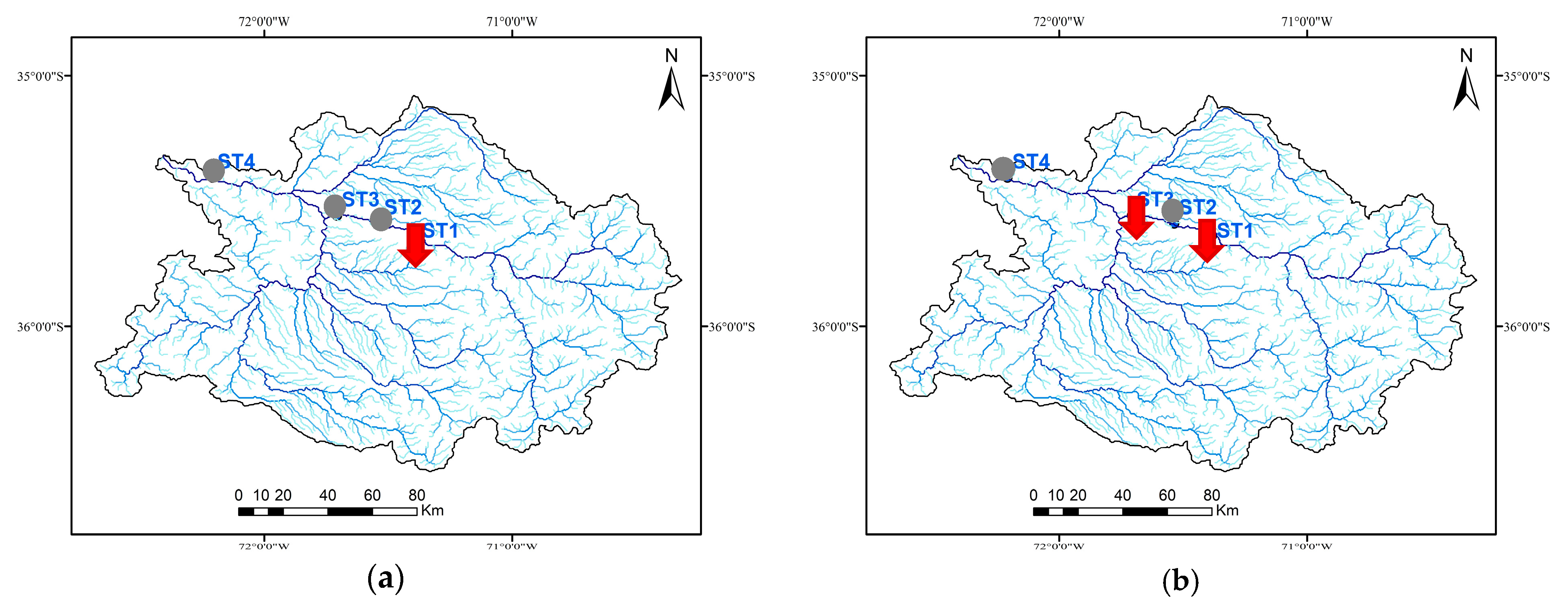
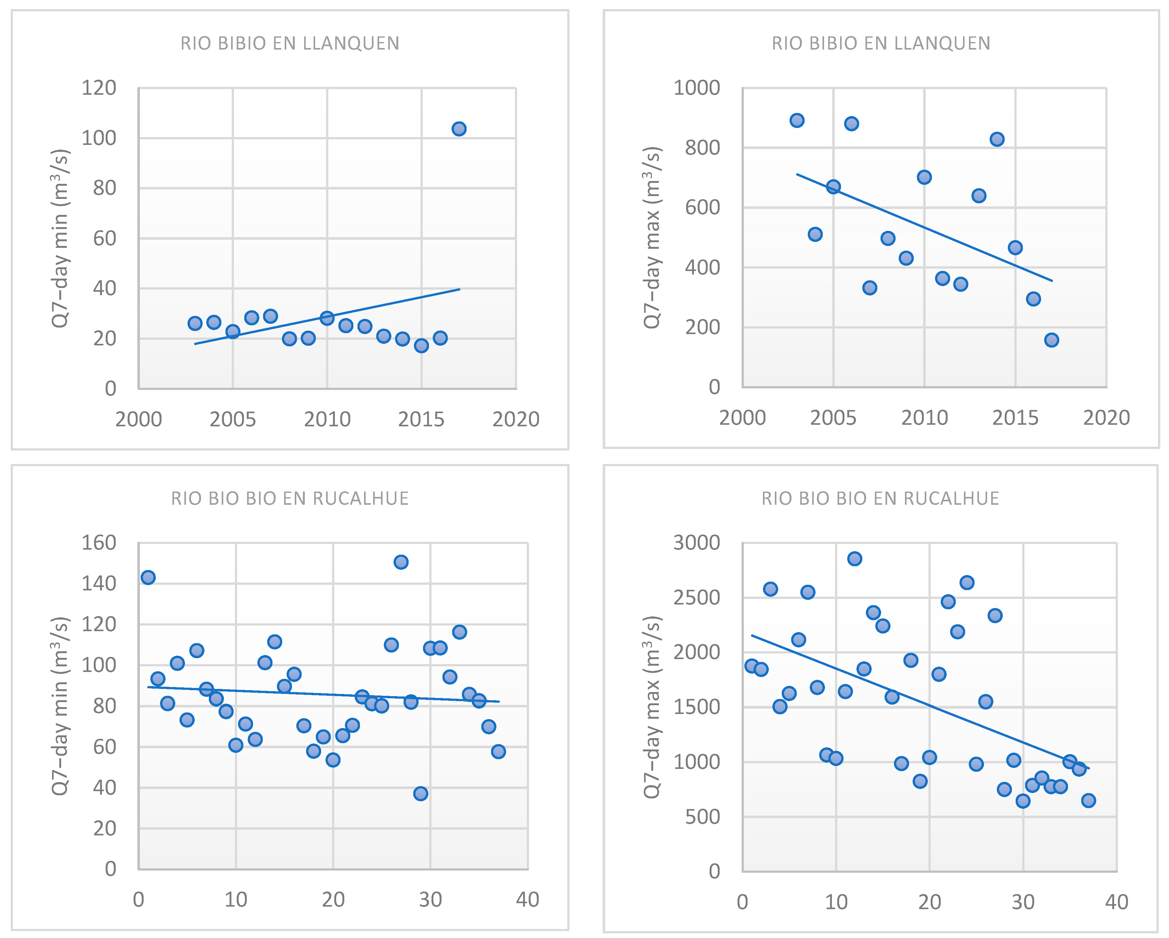
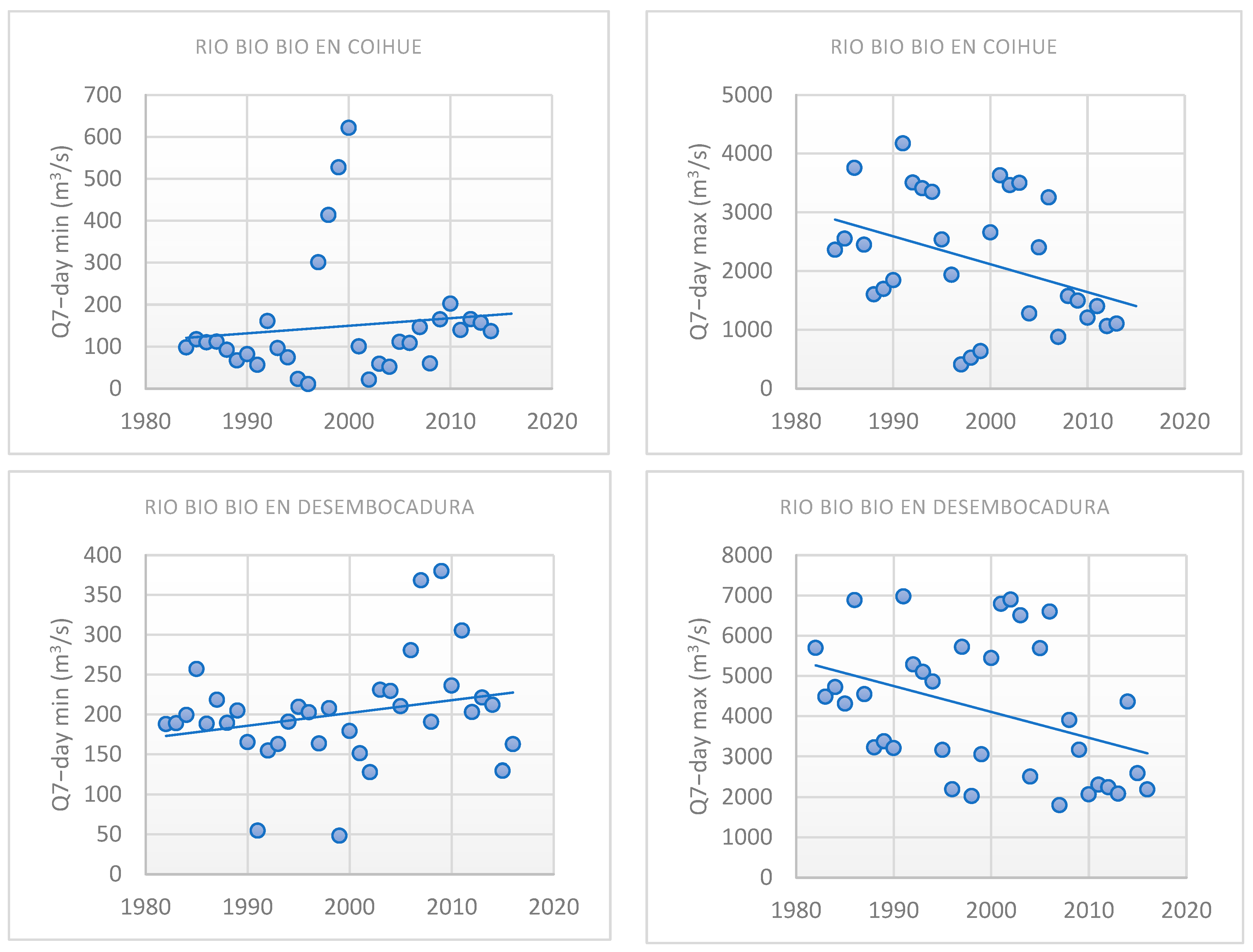
3.1.4. Biobío River Basin

The hydrological trends in the Biobío river basin were analyzed across four stations: Río Biobío en Llanquén, Río Biobío en Rucalhue, Río Biobío en Coihue, and Río Biobío en Desembocadura (

Table 6. Trends and normality tests of low and high-flow time series for the Biobío River.

Station Name	Río Biobío En Llanquén				Station Name	Río Biobío En Rucalhue
Indices (m3/s)	Norm Test Result	Flow Range m3/s	Slope	p-Value	Indices (m3/s)	Norm Test Result	Flow Range m3/s	Slope	p-Value
1-day min	normal	16.80–95.20	1.396	0.250	1-day min	normal	29.30–135	−0.62	0.100
3-day min	normal	16.95–96.97	1.417	0.250	3-day min	normal	33.07–137.3	−0.309	0.500
7-day min	normal	17.14–103.6	1.552	0.250	7-day min	normal	37.03–150.6	0.147	0.500
30-day min	normal	18.61–114	1.674	0.250	30-day min	normal	45.73–166.7	0.379	0.500
90-day min	normal	20.34–114	1.458	0.500	90-day min	normal	68.89–234.9	0.133	0.500
1-day max	normal	174.0–1592	−46.38	0.100	1-day max	normal	701.0–5589	−58.6	0.005
3-day max	normal	163.7–1292	−38.46	0.050	3-day max	normal	667.3–3824	−48.42	0.001
7-day max	normal	157.0–891.1	−25.39	0.010	7-day max	normal	643.7–2855	−35.92	0.001
30-day max	normal	130.9–603.1	−13.97	0.025	30-day max	normal	545.0–1612	−18.46	0.001
90-day max	normal	119.6–418.7	−9.497	0.010	90-day max	normal	448.1–1252	−11.98	0.001
Station Name	Río Biobío En Coihue				Station Name	Río Biobío En Desembocadura
Indices (m3/s)	Norm Test Result	Flow Range m3/s	Slope	p-Value	Indices (m3/s)	Norm Test Result	Flow Range m3/s	Slope	p-Value
1-day min	normal	10.6–526.1	1.278	0.500	1-day min	normal	32.60–349.0	1.041	0.500
3-day min	normal	10.6–551.7	1.538	0.500	3-day min	normal	46.83–355.4	1.364	0.250
7-day min	normal	10.6–621.6	1.806	0.500	7-day min	normal	48.41–380.0	1.600	0.250
30-day min	normal	15.97–643.8	2.391	0.500	30-day min	normal	51.93–460.5	1.805	0.250
90-day min	normal	49.19–653.1	2.174	0.500	90-day min	normal	77.56–553.5	2.393	0.250
1-day max	normal	412.7–7372	−63.8	0.250	1-day max	normal	2367–13,750	−97.25	0.050
3-day max	normal	412.4–6388	−52.59	0.100	3-day max	normal	1994–9877	−80.58	0.050
7-day max	normal	411.7–4175	−40.89	0.100	7-day max	normal	1798–6974	−64.31	0.025
30-day max	normal	408.2–2542	−13.24	0.500	30-day max	normal	1217–4600	−31.56	0.025
90-day max	normal	398.9–1998	−7.056	0.500	90-day max	normal	774–3375	−20.71	0.050

). The low-flow indices generally showed slight increases, and the high-flow indices displayed significant declines across most stations. All examined indicators followed a normal distribution.

At the Río Biobío en Llanquén station, the low-flow indices showed increasing trends that were not statistically significant, such as the 90-day minimum flow, with a positive slope of 1.458 (p-value of 0.5). In contrast, the high flows exhibited a declining trend, with the 30-day maximum flow showing a slope of −13.97 (p-value of 0.025).

At Río Biobío en Rucalhue, the low-flow conditions remained stable, with minimal changes. For instance, the 7-day minimum flow showed no significant variation (slope of 0.147 and p-value of 0.5). Conversely, the high flows exhibited a significant reduction, as the 3-day maximum flow declined sharply (slope of −48.42 and p-value of 0.001).

Río Biobío en Coihue displayed a notable increase in low flows, though not statistically significant, with the 90-day minimum flow having a positive slope of 2.174 (p-value of 0.5). In contrast, the high flows showed a decrease, with the 7-day maximum flow presenting a consistent negative slope of −40.89 (p-value of 0.1).

Finally, at Río Biobío en Desembocadura, slight increases were observed in low-flow indices, though not statistically significant, including the 90-day minimum flow, which showed a slope of 2.393 (p-value of 0.25). On the other hand, high flows recorded significant declines, with the 1-day maximum flow exhibiting a slope of −97.25 (p-value of 0.05).

The 7-day minimum and maximum flow plots for the Biobío River (Figure 8) confirm the trends observed in Table 6. There were non-significant increases in low flows across all the stations. High flows show significant decreases at all stations, except Biobío En Coihue.

These findings are supported by the spatial representation of the low- and high-flow trends in the river basin (Figure 9), where the low flows at all stations display non-significant trends. However, high flows show significant decreases at most stations.

3.2. Baseflow Index (BFI)

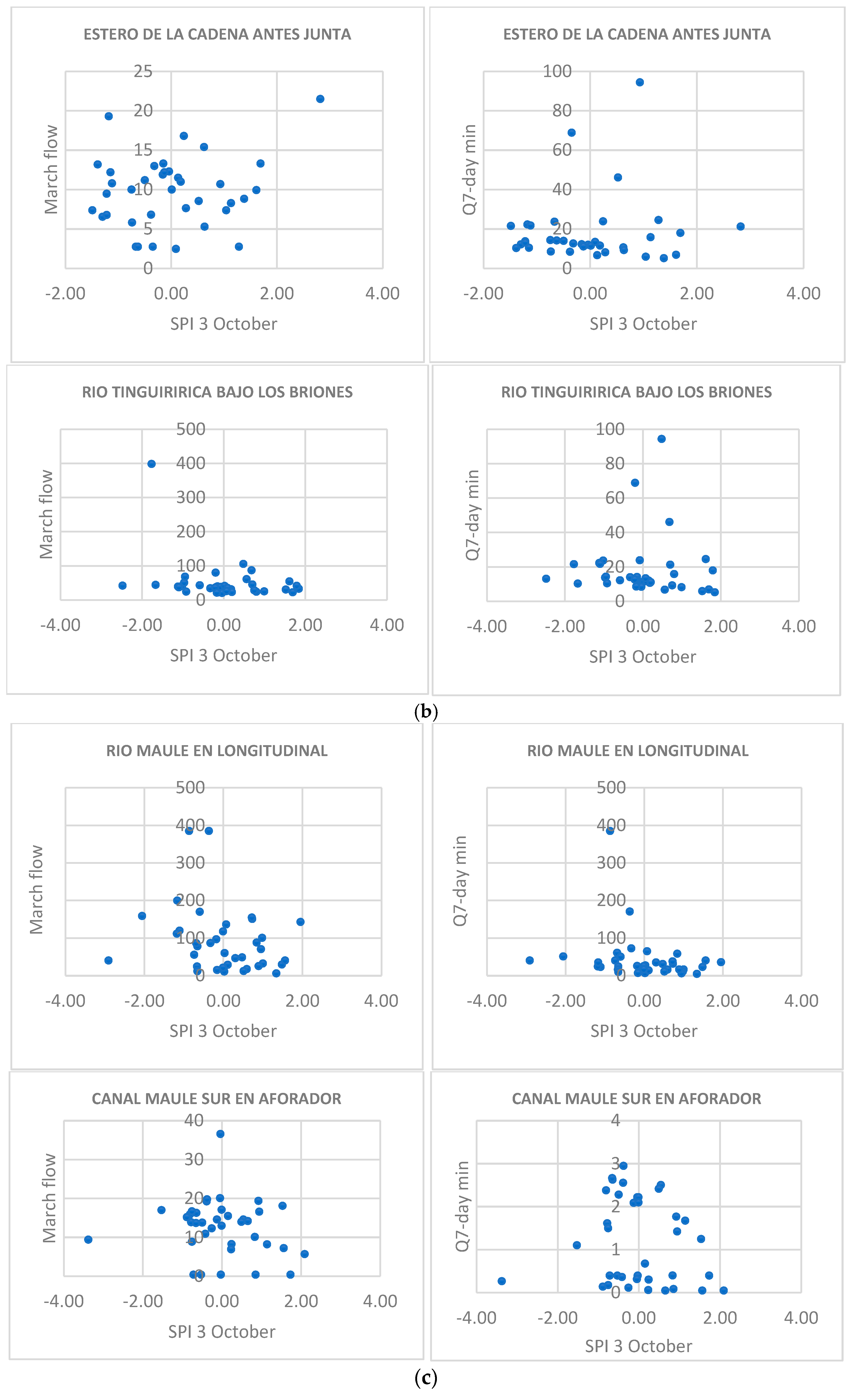
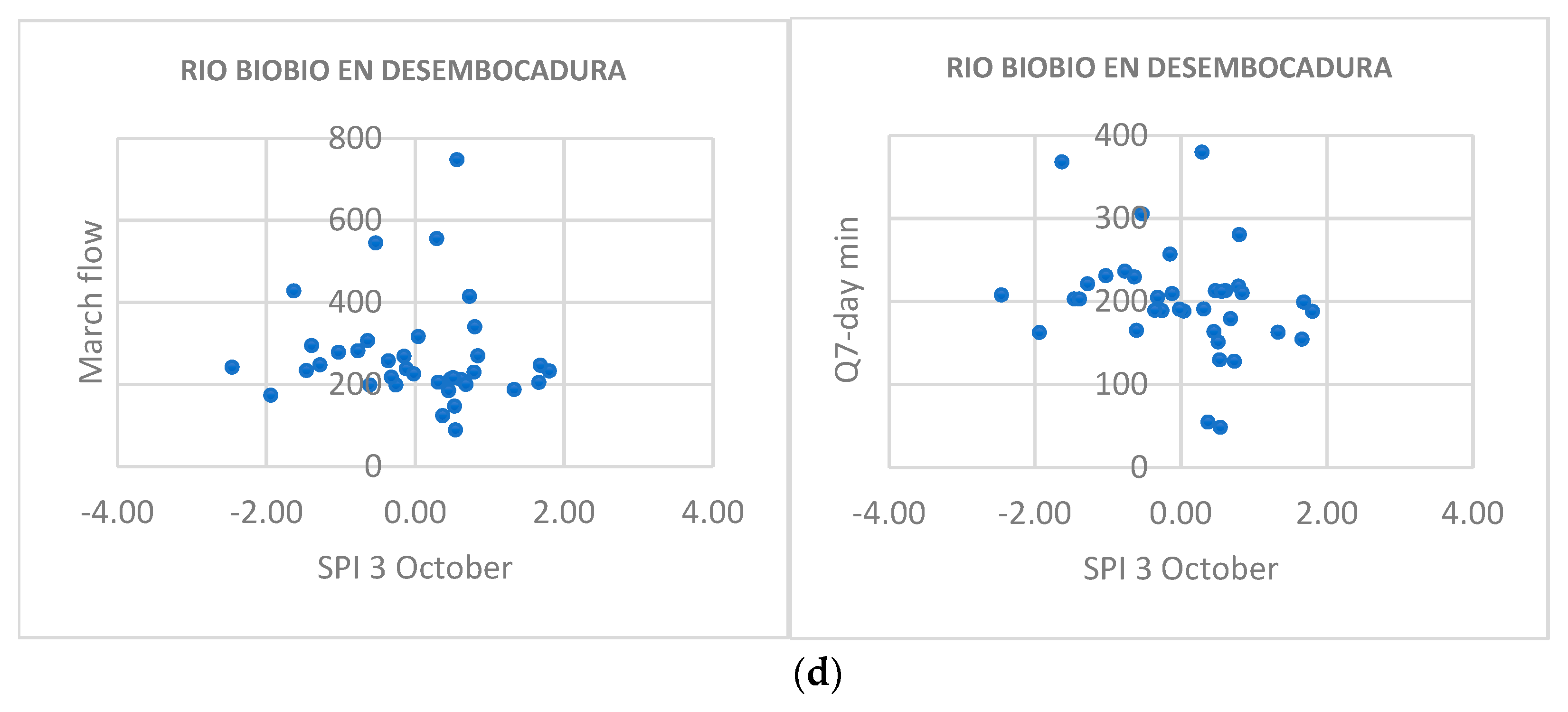
The average baseflow index was calculated for each of the hydrometric stations in the four river basins. The stations are distributed from the upstream to the downstream sections of each river, to reflect the spatial variations in groundwater contributions (

Table 7. Base flow index of the river basins.

	ST1	ST2	ST3	ST4	ST5	ST6
Maipo	0.90	0.82	0.84	0.67	0.87	0.88
Rapel	0.65	0.77	0.82	0.68	-	-
Maule	0.70	0.90	0.65	0.70	-	-
Biobío	0.68	0.71	0.75	0.74	-	-

).

The Maipo River shows the strongest baseflow influence, with consistently high BFI values that range from 0.90 at the upstream station (ST1: Río Maipo en Las Hualtatas) to 0.88 at the downstream station (ST6: Río Maipo en El Manzano). The values progressively decrease to 0.67 at ST4 (Río Olivares antes junta Colorado), before rising again (0.87) at ST5 (Río Colorado antes junta Río Maipo) and (0.88) at ST6 (Río Maipo en El Manzano). The above can be explained by the fact that the stations used for the flow evaluation in the Maipo River are located in the mid-to-upper part of the basin (Figure 3), where there is a significant snowmelt influence. In fact, the hydrological regime of the station Río Maipo en El Manzano is classified as nival [47].

The BFI values for the Rapel River show variation in the baseflow contributions along the river, ranging from 0.65 at the upstream station (ST1: Cachapoal en puente Termas de Cauquenes) to 0.68 at the downstream station (ST4: Río Tinguirririca en Los Olmos). The two upstream stations (ST1 and ST2), located in the pre-cordilleran zone, are influenced by snowmelt, which contributes to sustained baseflow. In contrast, the two downstream stations (ST3 and ST4) located in the central valley are more influenced by precipitation. The results highlight the transition from a snowmelt-driven system in the upper basin to a rainfall system in the lower basin, as indicated by Salcedo-Castro et al. [48], who described the Rapel River basin as exhibiting a mixed hydrological regime.

The Maule River shows a range of BFI values, with the high value recorded at ST2 (Canal Duao Zapata) at 0.90 and a decline to 0.65 at ST3 (Río Maule en Longitudinal), before slightly increasing to 0.70 at ST4 (Río Maule en Forel). The two upstream stations are related to irrigation canals, which are managed by irrigators, and their flow regime corresponds to irrigation needs rather than climatic conditions. These management practices may contribute to the inconsistency in the BFI values. The downstream stations (ST3 and ST4) represent more natural baseflow conditions, with values around 0.7, and are influenced by both surface and groundwater contributions.

The BFI values of the Biobío River range from 0.68 at ST1(Río Biobío en Llanquén) to 0.74 at ST4 (Río Biobío en Desembocadura), with the baseflow contributions being comparatively constant across the river. The low variation in BFI can be explained by the flow control exerted by large dams located in the upper part of the basin [49], especially during the dry season. In some analyzed cases, an increase in minimum flows is observed, as indicated by the trends shown in the graphs in Figure 8 for the 7-day min indicators.

The values of the baseflow index range from 65% to 90%, indicating that a significant proportion of river flow is derived from baseflow contributions. This shows that none of the rivers are intermittent and that they can maintain their flow during dry seasons. These results of the BFI values for all of the rivers examined show that the baseflow represents a fairly large percentage of the total runoff, suggesting that groundwater and snowmelt play a significant role in sustaining river flows in these basins and, therefore, for the fluvial ecosystem.

3.3. SPI Index

In order to gain a more comprehensive understanding of low flows in the basins, the SPI index was calculated for the basin area corresponding to each river flow station. This method helps identify the rainfall trends over the respective time series (1980–2016) and evaluate the potential for drought during this period. The data used correspond to the daily average rainfall from two rainfall stations per basin.

The plots show the correlation between SPI3 October and the March river flow, which marks the end of the dry season in the Southern Hemisphere, and also the Q7-day minimum low-flow values recorded at hydrological stations near meteorological stations. SPI3 represents the standardized precipitation index for the three-month August–October period, reflecting cumulative precipitation trends before the beginning of the dry season.

The results demonstrated a weak or non-significant correlation between SPI3 October and both March flows and 7-day minimum flows across all stations (Figure 10). In all four river basins, the flows remain within a consistent range regardless of drought or wet periods, as shown by the scattered data points, indicating the limited role of short-term precipitation variability and highlighting the influence of other factors, such as anthropogenic activities [50] and snowfall from the previous winter that determines how much meltwater contributes to river flows in the dry season. Summer storms in the upper areas of the river’s basin may bring localized heavy rainfall and temporarily increase river flows, even in the dry season. Also, rivers like Maule and Biobío are regulated by reservoirs like Laguna del Maule and Colbún (Maule River Basin) and Ralco-Pangue and Laguna del Laja (Biobío River Basin), which influences when and how much water is stored or released.

4. Discussions

The hydrological trends in the Maipo, Rapel, Maule, and Biobío Mediterranean basins highlight the combined climate variability (ENSO, PEO, and climate change) and anthropogenic activities on water resources. Central Chile’s Mediterranean climate is particularly sensitive to prolonged droughts, reduced precipitation, and rising temperatures [51,52]. The 2023 IPCC synthesis report indicates that the global water cycle is becoming more intense, with a notable decline in precipitation and snowpack across these regions [1]. In addition, snowmelt from the Andes, a key contributor to runoff during spring and summer, has fallen by as much as 30% in Chile due to the ongoing megadrought that started in 2010 [53]. Consistent with global trends observed in snow-fed river basins under climate change, these interacting factors further exacerbate the reduction in both low and high flows [1,54].

Anthropogenic factors further intensify these declines. Agriculture remains the predominant water user in the basins, particularly in the Rapel and Maipo rivers, where irrigation accounts for 93% and 61.6% of total water use, respectively [34,35]. Excessive water withdrawal for irrigation during dry periods is widely recognized as a major factor in the significant depletion of river flows, heightening competition among agricultural, urban, and industrial sectors [55,56]. Similar trends have been shown in other Andean basins, where growing agricultural demands aggravate water scarcity, especially with the reduction in snowmelt contributions [57]. These dynamics are driven by high demand for water in urban areas, (e.g., 659,893 Mm³/year in the Maipo basin), especially during droughts. Other significant impacts on water availability come from the mining sector, particularly in the Maipo and Rapel River basins. Mining operations require large volumes of water for extraction and processing, creating additional pressure on water resources, in terms of quantity and quality, and intensifying conflicts between mining, agriculture, and urban uses [58,59].

Low flows at most stations on the Maipo River showed significant decreases, indicating that the river is under pressure from urban and agricultural demands, hydroelectricity, and mining, but the upstream stations showed non-significant trends, which may be due to groundwater contributions. For the Maule and Rapel River basins, only the upstream Maule and downstream Rapel stations showed a significant decrease, and for the other stations, non-significant decreasing trends were observed, suggesting that some river reaches are more vulnerable than others. The spatial variability of these trends indicates a combination of surface and groundwater contributions, hydropower, and irrigation regulations. For example, on the Maule River, where there are no strong decreasing trends, the Duao Zapata station can only operate during the irrigation season, and their flow regime is controlled by the farmers at the intakes. But this does not reflect the annual trends, and also, in times of drought, the DGA can intervene at the intakes and reduce the incoming flows. In contrast, the Canal Maule Sur en Aforador station shows significant declines, which is controlled by a reservoir or dam operation upstream. These results highlight the impact of human water management practices on hydrological flow trends.

Hydropower dam regulation has a significant impact on river flow patterns. In basins like the Rapel, Maule, and Biobío, hydropower infrastructure alters the natural flow regime to produce energy. For instance, the Biobío River has 17 plants supplying more than 2800 MW [37], and the Rapel River, with 26 plants, produces more than 1033 MW [28] and experiences reduced high-flow discharges due to water regulation of the reservoirs. Similarly, the Maule basin, where hydropower production (447.01 m³/s) constitutes a major water-dependent use [33], significant flow alterations are also evident.

In the Rapel River basin, a significant reduction in high flows is observed at upstream stations, likely due to reduced precipitation. In contrast, downstream stations show stable trends suggesting that groundwater contributions and reservoir releases may help to stabilize high-flow variability. Similarly, in the Biobío River basin, where hydropower operations are extensive, the weak increasing trends in low flows, although not statistically significant, suggest a stabilization of baseflows through controlled reservoir releases. This highlights the importance of groundwater and flow regulation in maintaining low flows [60]. While hydropower is important for advancing renewable energy goals, it disrupts sediment transport, affects downstream ecosystems, and decreases the natural variability of river flow regimes [18,61,62].

On a global scale, the trends observed in Chile align with those in other regions with Mediterranean climates, where declining rainfall, land use changes, and intensive water use have led to significant reductions in river flow [1,53,63]. Such changes are compounded by the impact of climate change on hydrological cycles, as highlighted by studies in Mediterranean basins, including the findings of the HyMeX program [64] and broader assessments of flooding processes and water scarcity under climate change scenarios [65]. Additionally, the combined effects of glacial retreat, land use intensification, and hydropower development mirror patterns observed in the Andes basins, where altered hydrological processes exacerbate water stress [66].

While the dynamics of surface water contributions are evident in the trends of low and high flows, groundwater interactions, as quantified by the BFI, must also be considered. The BFI underscores the critical role of groundwater in sustaining river flows during dry spells and extreme weather events, providing valuable insights into the hydrological resilience of rivers under seasonal and climatic variations [67].

The high BFI values observed for the Maipo River indicate a clear dependence on groundwater contributions, which help to protect the river against short-term hydrological fluctuations and reduce the impact of decreasing snowmelt and precipitation, factors characteristic of declining trends in Central Chile [53]. Conversely, the variations in BFI values in the Rapel and Maule Rivers suggest a mixed contribution of surface and groundwater, and their interaction, making these basins more vulnerable to seasonal precipitation patterns and human activity. Recent studies [50] reveal that urban water extraction and mainly agricultural water use have a significant impact on streamflow in Chile’s main river basins, exacerbating this sensitivity.

In the Biobío River basin, consistently high and stable BFI values indicate that river flows achieved a stabilization face to climatic variability, confirming the similar resilience observed in studies carried out in regions where groundwater recharge and snowmelt in the Andes significantly influence river flow [68]. This aligns with the observed trends in low flows, which show non-significant increases. Studies on the Maipo River further underline the contribution of glacial meltwater, which interacts with groundwater to sustain river flows during periods of drought [68]. These BFI variations are consistent with global findings, indicating that human activities, particularly agriculture, urban growth, and industrial activities, are significant to reduced river flow [50].

The weak correlation aligns with the observation of flow trends and BFI. For rivers with high BFI values, such as the Maipo and Biobío, groundwater contributions could sustain flows during dry periods, reducing the effects of precipitation variability. Rivers with more variability in BFI values, like the Rapel River and portions of the Maule River, are more susceptible to seasonal precipitation fluctuations due to human activities like irrigation and hydropower [50,69].

The complexity of the relationship between precipitation and river flow regimes is heightened by the influence of the El Niño–Southern Oscillation (ENSO), which can enhance rainfall and temporarily increase river flows, whereas La Niña phases typically extend dry periods and reduce streamflow [53,70]. However, the lack of a significant correlation between the BFI and SPI3 with river flows (March flow and 7-day min) suggests that groundwater storage and snowmelt function as important buffers, mitigating the immediate effects of the precipitation anomalies induced by ENSO. These findings align with further studies that demonstrate how resilient groundwater and snow-fed systems are to short-term climate variability [66].

The results further highlight the critical role of human activities in decoupling the relationship between precipitation and river flow regime. On the one hand, hydropower regulation, particularly in the Rapel [18] and Biobío basins [49], supports the maintenance of low flows through controlled releases. On the other hand, it restricts the natural variability of high flow [60]. In addition, the growing demands for irrigation and urban water, especially in the Maipo and Rapel basins, exacerbate flow variability by increasing water extraction during dry periods [50,55]. The findings from low-flow analysis of the Chilean rivers are in agreement with the findings of studies about the low-flow trends of German rivers, revealing the strong contribution of human impact in river basin management [71].

5. Conclusions

This study is a comprehensive overview of the hydrologic responses of the four rivers in Chile based on a combined assessment of flow trends, BFI, and SPI3 in October. Decreasing trends in low and high flows have revealed the significant impacts of climate change, reduced precipitation, and snowpack variability on river runoff.

The spatial variability observed between the river basins is evident, especially at the Maipo River, which shows notable drops in low flow due to agricultural and urban water demands. The fact that these drops occur when BFI values are high suggests that, while groundwater buffering mitigates some impacts, it cannot counter surface runoff drops during prolonged droughts. In contrast, the Rapel and Maule Rivers exhibit non-significant decreasing trends in low flows in most stations, with only one station showing a significant decrease, in line with their moderate and variable BFI values. This shows that groundwater contributions and surface runoff are balanced, with hydropower regulation stabilizing flows. The Biobío River shows stable values of BFI, indicating a system buffered by groundwater, but also subject to the influences of surface processes under a wide range of conditions, particularly as low-flow trends increase in the presence of statistical insignificance. This complements the SPI3 findings, which find a weak correlation between precipitation and flow, highlighting that precipitation variability does not have a strong effect on streamflow and confirming that snowmelt, groundwater contributions, and anthropogenic activities, such as hydropower regulation, are modeling the flow regime in the river.

All of these results show how different factors influence river behavior, emphasizing the necessity of integrated water resource management, but with different approaches to deal with the combined impacts of human demands and climatic variability.

References

1. IPCC. Summary for Policymakers. In Climate Change 2023: Synthesis Report. Contribution of Working Groups I, II and III to the Sixth Assessment Report of the Intergovernmental Panel on Climate Change; Core Writing Team, Lee, H., Romero, J., Eds.; Intergovernmental Panel on Climate Change (IPCC): Geneva, Switzerland, 2023. [Google Scholar] [CrossRef]
2. MacAlister, C.; Baggio, G.; Perera, D.; Qadir, M.; Taing, L.; Smakhtin, V. Global Water Security 2023 Assessment; United Nations, University Institute for Water, Environment and Health: Hamilton, ON, Canada, 2023. [Google Scholar]
3. OECD. Water Governance in OECD Countries: A Multi-Level Approach; OECD Publishing: Paris, France, 2011. [Google Scholar]
4. Agarwal, A.; de los Angeles, M.; Bhatia, R.; Chéret, I.; Davila-Poblete, S.; Falkenmark, M.; Gonzalez Villareal, F.; Jønch-Clausen, T.; Ait Kadi, M.; Kindler, J. Integrated Water Resources Management; Global Water Partnership: Stockholm, Sweden, 2000. [Google Scholar]
5. Stewart, B. Measuring what we manage–the importance of hydrological data to water resources management. Proc. Int. Assoc. Hydrol. Sci. 2015, 366, 80–85. [Google Scholar] [CrossRef]
6. Ghannem, S.; Bergillos, R.J.; Paredes-Arquiola, J.; Martínez-Capel, F.; Andreu, J. Coupling hydrological, habitat and water supply indicators to improve the management of environmental flows. Sci. Total Environ. 2023, 898, 165640. [Google Scholar] [CrossRef] [PubMed]
7. OECD. OECD Principles on Water Governance; OECD Water Governance Programme: Paris, France, 2015. [Google Scholar]
8. Grantham, T.E.; Figueroa, R.; Prat, N. Water management in mediterranean river basins: A comparison of management frameworks, physical impacts, and ecological responses. Hydrobiologia 2013, 719, 451–482. [Google Scholar] [CrossRef]
9. Andrew, J.T.; Sauquet, E. Climate change impacts and water management adaptation in two mediterranean-climate watersheds: Learning from the Durance and Sacramento Rivers. Water 2017, 9, 126. [Google Scholar] [CrossRef]
10. Figueroa, R.; Bónada, N.; Guevara, M.; Pedreros, P.; Correa-Araneda, F.; Díaz, M.E.; Ruiz, V.H. Freshwater biodiversity and conservation in mediterranean climate streams of Chile. Hydrobiologia 2013, 719, 269–289. [Google Scholar] [CrossRef]
11. Armesto, J.J.; Arroyo, M.T.K.; Hinojosa, L.F. The mediterranean environment of Chile. In The Physical Geography of South America; Veblen Thomas, T., Young Kenneth, R., Orme Antony, R., Eds.; Universidad de Chile: Santiago, Chile, 2007. [Google Scholar]
12. World Bank Group. Climate Risk Country Profile: Chile. 2021. Available online: https://climateknowledgeportal.worldbank.org/country/chile/climate-data-historical (accessed on 3 January 2025).
13. Niemeyer, H.; Cereceda, P. Geografía de Chile. Tomo VIII Hidrografía; Instituto Geográfico Militar: Santiago, Chile, 1989. [Google Scholar]
14. Fuentes, E. Sinopsis de paisajes de Chile central. In Ecología del Paisaje en Chile Central Estudios sobre sus Espacios Montañosos; Fuentes, E., Prenafeta, S., Eds.; Universidad Católica de Chile: Santiago, Chile, 1988; pp. 17–27. [Google Scholar]
15. Garreaud, R.D.; Alvarez-Garreton, C.; Barichivich, J.; Boisier, J.P.; Christie, D.; Galleguillos, M.; LeQuesne, C.; McPhee, J.; Zambrano-Bigiarini, M. The 2010–2015 megadrought in central Chile: Impacts on regional hydroclimate and vegetation. Hydrol. Earth Syst. Sci. 2017, 21, 6307–6327. [Google Scholar] [CrossRef]
16. Grafton, R.Q.; Pittock, J.; Davis, R.; Williams, J.; Fu, G.; Warburton, M.; Udall, B.; McKenzie, R.; Yu, X.; Che, N.; et al. Global insights into water resources, climate change and governance. Nat. Clim. Change 2013, 3, 315–321. [Google Scholar] [CrossRef]
17. Rivera, R.; Leal, C.; Barra, R.O. Toward Water Security (SDG 6) amidst the Climate and Water Crisis: Lessons from Chile. Environ. Sci. Technol. 2023, 57, 12940–12943. [Google Scholar] [CrossRef]
18. Alcayaga, H.; Palma, S.; Caamaño, D.; Mao, L.; Soto-Alvarez, M. Detecting and quantifying hydromorphology changes in a chilean river after 50 years of dam operation. J. S. Am. Earth Sci. 2019, 93, 253–266. [Google Scholar] [CrossRef]
19. Dirección General de Aguas. Atlas del Agua; Ministerio de Obras Públicas: Santiago, Chile, 2016. [Google Scholar]
20. Vicuña, S.; Bustos, E. Vulnerability and Adaptation to Climate Variability and Change in the Maipo Basin, Central Chile. Final Technical Report. 2016. Available online: https://cambioglobal.uc.cl/wp-content/uploads/2023/09/Informe_Tecnico_Final_Proyecto_MAPA-Maipo_Plan_de_Adaptacion.pdf (accessed on 17 February 2025).
21. Dirección General de Aguas. Diagnostico y Clasificacion de los Cursos y Cuerpos de Agua Segun Objetivos de Calidad. Cuenca del río Rapel. 2004. Available online: https://mma.gob.cl/wp-content/uploads/2017/12/Rapel.pdf (accessed on 15 December 2024).
22. Roco, L.; Poblete, D.; Meza, F.; Kerrigan, G. Farmers’ options to address water scarcity in a changing climate: Case studies from two basins in Mediterranean Chile. Environ. Manag. 2016, 58, 958–971. [Google Scholar] [CrossRef]
23. Elgueta, A.; Thoms, M.C.; Górski, K.; Díaz, G.; Habit, E.M. Functional process zones and their fish communities in temperate Andean river networks. River Res. Appl. 2019, 35, 1702–1711. [Google Scholar] [CrossRef]
24. Escenarios Hidricos 2030. Maipo Resiliente, de la Crisis a la Regeneración Hídrica en la Cuenca del Río Maipo; Fundación Chile: Santiago, Chile, 2024. [Google Scholar]
25. BCN. Hidrografía Región del Maule. Biblioteca del Congreso Nacional de Chile. 2017. Available online: https://www.bcn.cl/siit/nuestropais/region7/hidrografia.htm (accessed on 10 December 2024).
26. Masotti, I.; Aparicio-Rizzo, P.; Yevenes, M.A.; Garreaud, R.; Belmar, L.; Farías, L. The influence of river discharge on nutrient export and phytoplankton biomass off the Central Chile coast (33–37 S): Seasonal cycle and interannual variability. Front. Mar. Sci. 2018, 5, 423. [Google Scholar] [CrossRef]
27. CIREN. Precordillera de Santiago-Cajón del Maipo. 2021. Available online: https://observatorio.ciren.cl/profile/clima/precordillera-santiago-cajon-del-maipo (accessed on 20 December 2024).
28. Bennison, G.; Rojas, R.; Claro, E.; Gálvez, V.; Bridgart, R.; Caroca, M. Gestión Integrada de Recursos Hídricos Cuenca del Río Rapel–Informe Final (Etapas 1 y 2); Fundación CSIRO Chile Research: Santiago, Chile, 2021. [Google Scholar]
29. Escenarios Hidricos 2030. Cuenca del río Maule. Available online: https://escenarioshidricos.cl/nuestro-trabajo/cuenca-del-rio-maule/ (accessed on 15 November 2024).
30. Universidad de Concepción-Departamento de Recursos Hídricos. Plan Estratégico de Gestión Hidrica En La Cuenca Del Biobío; Dirección General de Aguas-Ministerio de Obras Públicas: Santiago, Chile, 2021. [Google Scholar]
31. Dirección General de Aguas. Inventario de Cuencas, Subcuencas y Subsubcuenas de Chile, Gobierno de Chile. Available online: https://bibliotecadigital.ciren.cl/items/d9c31b57-5479-49d3-af64-d03e6a374b1a (accessed on 22 November 2024).
32. Instituto Nacional de Estadísticas. Síntesis de Resultados. Censo 2017; Instituto Nacional de Estadísticas: Santiago, Chile, 2018. [Google Scholar]
33. Vicuña, S.; Bustos, E. Plan Estratégico de Gestión Hídrica en la Cuenca del Maule; DGA-División de Estudios y Planificación: Santiago, Chile, 2020. [Google Scholar]
34. Dirección General de Aguas. Estimación de la Demanda Actual, Proyecciones Futuras y Caracterización de la Calidad de Los Recursos Hídricos en Chile; Ministerio de Obras Públicas: Santiago, Chile, 2017. [Google Scholar]
35. Fundación Chile. Reporte Huella hídrica en Chile. Sectores Prioritarios de la Cuenca del río Rapel; Fundación Chile: Santiago, Chile, 2015. [Google Scholar]
36. Barría, P.; Rojas, M.; Moraga, P.; Muñoz, A.; Bozkurt, D.; Alvarez-Garreton, C. Anthropocene and streamflow: Long-term perspective of streamflow variability and water rights. Elem. Sci. Anthr. 2019, 7, 2. [Google Scholar] [CrossRef]
37. Figueroa, R.; Parra, O.; Díaz, M.E. La cuenca hidrográfica del río Biobío. In Centro EULA Evoución y Perspectivas a 30 años de su Creación; Universidad de Concepción: Concepción, Chile, 2020; pp. 91–138. [Google Scholar]
38. Bormann, H.; Pinter, N.; Elfert, S. Hydrological signatures of flood trends on German rivers: Flood frequencies, flood heights and specific stages. J. Hydrol. 2011, 404, 50–66. [Google Scholar] [CrossRef]
39. Richter, B.D.; Baumgartner, J.V.; Powell, J.; Braun, D.P. A method for assessing hydrologic alteration within ecosystems. Conserv. Biol. 1996, 10, 1163–1174. [Google Scholar] [CrossRef]
40. Richter, B.D.; Baumgartner, J.V.; Wigington, R.; Braun, D. How much water does a river need? Freshw. Biol. 1997, 37, 231–249. [Google Scholar] [CrossRef]
41. Olden, J.D.; Poff, N.L. Redundancy and the choice of hydrologic indices for characterizing streamflow regimes. River Res. Appl. 2003, 19, 101–121. [Google Scholar] [CrossRef]
42. Xiong, B.; Xiong, L.; Chen, J.; Xu, C.-Y.; Li, L. Multiple causes of nonstationarity in the Weihe annual low-flow series. Hydrol. Earth Syst. Sci. 2018, 22, 1525–1542. [Google Scholar] [CrossRef]
43. Jelovčan, M.; Šraj, M. Comprehensive low-flow analysis of the Vipava river. Acta Geogr. Slov. 2022, 62, 37–53. [Google Scholar] [CrossRef]
44. Massey, F.J., Jr. The Kolmogorov-Smirnov test for goodness of fit. J. Am. Stat. Assoc. 1951, 46, 68–78. [Google Scholar] [CrossRef]
45. Kendall, M.G. Rank Correlation Methods; Griffin: London, UK, 1975. [Google Scholar]
46. McKee, T.B.; Doesken, N.J.; Kleist, J. The relationship of drought frequency and duration to time scales. In Proceedings of the 8th Conference on Applied Climatology, Anaheim, CA, USA, 17–22 January 1993; pp. 179–183. [Google Scholar]
47. CADE-IDEPE. Diagnóstico y Clasificación de los Cursos y Cuerpos de Agua Según Objetivos de Calidad: Informe Final, año 2004; Dirección General de Aguas: Santiago, Chile, 2004. [Google Scholar]
48. Salcedo-Castro, J.; Olita, A.; Saavedra, F.; Saldías, G.S.; Cruz-Gómez, R.C.; De La Torre Martínez, C.D. Modeling the interannual variability in Maipo and Rapel river plumes off central Chile. Ocean Sci. 2023, 19, 1687–1703. [Google Scholar] [CrossRef]
49. Villablanca, L.; Batalla, R.J.; Piqué, G.; Iroumé, A. Hydrological effects of large dams in Chilean rivers. J. Hydrol. Reg. Stud. 2022, 41, 101060. [Google Scholar] [CrossRef]
50. Álamos, N.; Alvarez-Garreton, C.; Muñoz, A.; González-Reyes, Á. The influence of human activities on streamflow reductions during the megadrought in central Chile. Hydrol. Earth Syst. Sci. 2024, 28, 2483–2503. [Google Scholar] [CrossRef]
51. Escanilla-Minchel, R.; Alcayaga, H.; Soto-Alvarez, M.; Kinnard, C.; Urrutia, R. Evaluation of the impact of climate change on runoff generation in an andean glacier watershed. Water 2020, 12, 3547. [Google Scholar] [CrossRef]
52. Cortés Gonzalez, A.C.; Alcayaga, H.; Escanilla-Minchel, R.; Aguayo, M.; Aguayo, M.; Orellana, C. Evaluation of the effects of climatic variabilities on future hydrological scenarios: Application to a coastal basin in Central Chile. Hydrol. Res. 2024, 55, 1197–1216. [Google Scholar] [CrossRef]
53. Garreaud, R.D.; Boisier, J.P.; Rondanelli, R.; Montecinos, A.; Sepúlveda, H.H.; Veloso-Aguila, D. The central Chile mega drought (2010–2018): A climate dynamics perspective. Int. J. Climatol. 2020, 40, 421–439. [Google Scholar] [CrossRef]
54. Masiokas, M.H.; Rabatel, A.; Rivera, A.; Ruiz, L.; Pitte, P.; Ceballos, J.L.; Barcaza, G.; Soruco, A.; Bown, F.; Berthier, E.; et al. A review of the current state and recent changes of the Andean cryosphere. Front. Earth Sci. 2020, 8, 1–27. [Google Scholar] [CrossRef]
55. Flörke, M.; Schneider, C.; McDonald, R.I. Water competition between cities and agriculture driven by climate change and urban growth. Nat. Sustain. 2018, 1, 51–58. [Google Scholar] [CrossRef]
56. Gleick, P.H. Water use. Annu. Rev. Environ. Resour. 2003, 28, 275–314. [Google Scholar] [CrossRef]
57. Vuille, M.; Carey, M.; Huggel, C.; Buytaert, W.; Rabatel, A.; Jacobsen, D.; Soruco, A.; Villacis, M.; Yarleque, C.; Timm, O.E.; et al. Rapid decline of snow and ice in the tropical Andes—Impacts, uncertainties and challenges ahead. Earth-Sci. Rev. 2018, 176, 195–213. [Google Scholar] [CrossRef]
58. Donoso, G. Water Policy in Chile; Global Issues in Water Policy Series Vol. 21; Springer International Publishing: Cham, Switzerland, 2018. [Google Scholar] [CrossRef]
59. Walters, J.P.; Alcayaga, H.; Busco, C.; Araya, T. Mapping and Managing Organization Objectives: A Case Study of the Alto Maipo Hydroelectric Project in Chile. J. Water Resour. Plan. Manag. 2021, 147, 5021022. [Google Scholar] [CrossRef]
60. Díaz, G.; Arriagada, P.; Górski, K.; Link, O.; Karelovic, B.; Gonzalez, J.; Habit, E. Fragmentation of Chilean Andean rivers: Expected effects of hydropower development. Rev. Chil. Hist. Nat. 2019, 92, 1. [Google Scholar] [CrossRef]
61. Poff, N.L.; Allan, J.D.; Bain, M.B.; Karr, J.R.; Prestegaard, K.L.; Richter, B.D.; Sparks, R.E.; Stromberg, J.C. The natural flow regime. Bioscience 1997, 47, 769–784. [Google Scholar] [CrossRef]
62. Bin Ashraf, F.; Haghighi, A.T.; Riml, J.; Alfredsen, K.; Koskela, J.J.; Kløve, B.; Marttila, H. Changes in short term river flow regulation and hydropeaking in Nordic rivers. Sci. Rep. 2018, 8, 17232. [Google Scholar] [CrossRef]
63. Vorosmarty, C.J.; Green, P.; Salisbury, J.; Lammers, R.B. Global water resources: Vulnerability from climate change and population growth. Science 2000, 289, 284–288. [Google Scholar] [CrossRef]
64. Drobinski, P.; Ducrocq, V.; Alpert, P.; Anagnostou, E.; Béranger, K.; Borga, M.; Braud, I.; Chanzy, A.; Davolio, S.; Delrieu, G.; et al. HyMeX: A 10-year multidisciplinary program on the Mediterranean water cycle. Bull. Am. Meteorol. Soc. 2014, 95, 1063–1082. [Google Scholar] [CrossRef]
65. Tramblay, Y.; Arnaud, P.; Artigue, G.; Lang, M.; Paquet, E.; Neppel, L.; Sauquet, E. Changes in Mediterranean flood processes and seasonality. Hydrol. Earth Syst. Sci. Discuss. 2023, 27, 2973–2987. [Google Scholar] [CrossRef]
66. Calizaya, E.; Mejía, A.; Barboza, E.; Calizaya, F.; Corroto, F.; Salas, R.; Vásquez, H.; Turpo, E. Modelling snowmelt runoff from tropical Andean glaciers under climate change scenarios in the Santa River sub-basin (Peru). Water 2021, 13, 3535. [Google Scholar] [CrossRef]
67. Alvarez-Garreton, C.; Boisier, J.P.; Garreaud, R.; Seibert, J.; Vis, M. Progressive water deficits during multiyear droughts in basins with long hydrological memory in Chile. Hydrol. Earth Syst. Sci. 2021, 25, 429–446. [Google Scholar] [CrossRef]
68. McCarthy, M.; Meier, F.; Fatichi, S.; Stocker, B.D.; Shaw, T.E.; Miles, E.; Dussaillant, I.; Pellicciotti, F. Glacier contributions to river discharge during the current Chilean megadrought. Earth’s Futur. 2022, 10, e2022EF002852. [Google Scholar] [CrossRef]
69. Bloomfield, J.P.; Gong, M.; Marchant, B.P.; Coxon, G.; Addor, N. How is Baseflow Index (BFI) impacted by water resource management practices? Hydrol. Earth Syst. Sci. 2021, 25, 5355–5379. [Google Scholar] [CrossRef]
70. Van Dongen, R.; Scherler, D.; Wendi, D.; Deal, E.; Mao, L.; Marwan, N.; Meier, C.I. El Niño Southern Oscillation (ENSO)-induced hydrological anomalies in central Chile. EGUsphere 2022, 2022, 1–31. [Google Scholar] [CrossRef]
71. Bormann, H.; Pinter, N. Trends in low flows of German rivers since 1950: Comparability of different low-flow indicators and their spatial patterns. River Res. Appl. 2017, 33, 1191–1204. [Google Scholar] [CrossRef]
Figure 1. Location of basins considering in this study.
Water 17 00791 g001
Figure 2. Observed trends in 7−day minimum and 7−day maximum flows in Maipo River.
Water 17 00791 g002aWater 17 00791 g002bWater 17 00791 g002c
Figure 3. Maipo River hydrometric stationsshowing statistically significant decreasing trends (red downward arrows) or no significant trends (grey circles) in (a) the 7−day minimum flow indicators and (b) 7−day maximum flow indicators.
Water 17 00791 g003
Figure 4. Observed trends in 7−day minimum and 7−day maximum flows in Rapel River.
Water 17 00791 g004
Figure 5. Rapel River hydrometric stations showing statistically significant decreasing trends (red downward arrows) or no significant trends (grey circles) in (a) the 7−day minimum flow indicators and (b) 7−day maximum flow indicators.
Water 17 00791 g005
Figure 6. Observed trends in 7−day minimum and 7−day maximum flows in Maule River.
Water 17 00791 g006aWater 17 00791 g006b
Figure 7. Maule River hydrometric stations showing statistically significant decreasing trends (red downward arrows), or no significant trends (grey circles) in (a) the 7−day minimum flow indicators and (b) 7−day maximum flow indicators.
Water 17 00791 g007
Figure 8. Observed trends in 7−day minimum and 7−day maximum flows in Biobío River.
Water 17 00791 g008aWater 17 00791 g008b
Figure 9. Biobío River hydrometric stations showing statistically significant decreasing trends (red downward arrows) or no significant trends (grey circles) in (a) the 7−day minimum flow indicators and (b) 7−day maximum flow indicators.
Water 17 00791 g009
Figure 10. SPI3 October vs. March flow (m3/s) and 7 days minimum flow (Q-7day min, m3/s) of (a) Maipo River; (b) Rapel River; (c) Maule River; (d) Biobío River.
Water 17 00791 g010aWater 17 00791 g010bWater 17 00791 g010c