Abstract
Since 2011, Sargassum seaweed has spread widely outside the Sargasso Sea, causing massive strandings on the coasts of the West Indies and Mexico, causing serious economic, ecological, and health problems. This Atlantic pelagic alga has the characteristic of moving in rafts. According to in situ observations, their size and shape can vary with the wind. To better understand the effect of wind on Sargassum coverage and aggregation size, we conducted a large temporal (2019–2022) and spatial scale study in the West Indies using OLCI/Sentinel-3 satellite imagery. During this period, a database of nearly 1 million Sentinel-3 aggregations, including their geometric and wind characteristics, was established. Analysis of the size distribution showed that wind has a dual effect on disaggregation and agglomeration depending on wind speed and aggregation size: (1) low winds favor agglomeration for the smallest aggregations and disaggregation for the largest aggregations; (2) high winds favor disaggregation for all aggregation sizes. In addition, topography also plays a role in size distribution: the Caribbean arc favors agglomeration over offshore zones, and coastal areas favor disaggregation over offshore zones.
1. Introduction
The Atlantic Sargassum algae of the genus Sargassum C. Agardh (Phaeophyceae, Fucales) have mainly been observed in the Sargasso Sea [1], located in the subtropical Atlantic gyre. However, since 2011, these brown macroalgae have been proliferating in a new area in the North Tropical Atlantic called “The Great Sargassum Belt” [2]. This area extends from the Gulf of Mexico to the West African coast through the Caribbean Sea. The coastlines in this area experience massive strandings during periods of strong proliferation of Sargassum [3,4,5,6,7]. These strandings harm the economy [8,9] and the ecology [10,11,12,13]. Furthermore, the toxic gases (hydrogen sulfide and ammonia) emitted when decomposing and the high concentrations of heavy metals accumulated are a threat to public health [14,15,16,17,18].
In the Sargasso Sea and “The Great Sargassum Belt”, Sargassum seaweed refers to three morphotypes: Sargassum natans I Parr, S. natans VIII Parra, and S. fluitans III Parr [19,20,21]. These algae spend their entire lives drifting at the surface of the oceans and can form floating rafts. Rafts observed in the open sea are arranged in windrows and patches that range in size from tens of m2 to several hundred km2 [22,23,24]. The processes involved in the aggregation and dispersal of Sargassum rafts are not fully understood. However, in-situ observations of rafts [23,25,26,27] indicate that wind may play a role in raft shape and distribution, with aggregations being more elongated and aligned with the wind direction or dispersed in windy conditions [23,24,27,28]. Elongated rafts in windy conditions can be associated with Langmuir cells, resulting from Langmuir circulation that occurs at the surface of the oceans under the influence of the winds [29]. In contrast, larger and circular rafts have been observed in calm ocean conditions [22].
Some studies have also investigated the effect of wind on Sargassum distribution using spectral imagery, which allows for the collection of more spatial and temporal data. From a single day’s observations, Marmorino et al. [28] used high-resolution (~3 m) airborne imagery to observe the disintegration of Sargassum drift lines caused by wind. On a larger temporal and spatial scale, Sosa-Gutierrez et al. [30] and Sun et al. [31], using the Moderate Resolution Imaging Spectroradiometer (MODIS) sensor or the combination of multi-sensor output with MODIS, the Visible Infrared Imaging Radiometer Suite (VIIRS), and the Ocean Land Color Instrument (OLCI), observed a decrease in Sargassum coverage in the tropical Atlantic during extreme wind events associated with tropical cyclones conditions. However, they focus on extreme wind events only, while lower wind regimes have been poorly investigated.
This study aims to investigate and generalize the effect of wind, in non-extreme conditions, on Sargassum coverage and the Sargassum aggregation distribution. We analyze the distribution and dynamics of Sargassum rafts, especially on their disaggregation and agglomeration, over a range of low to moderate wind speeds (2 to 12 m·s−1) using OLCI. The spatial resolution of the OLCI (300 m) allowed us to observe Sargassum aggregations (i.e., sets of rafts), while a MODIS resolution of 1 km did not. Furthermore, the short revisit time of 1 to 2 days provides good spatial coverage and temporal sampling. In the current analysis, four years of Sargassum and wind data in the West Indies at the Lesser Antilles Arc location, an area heavily affected by Sargassum inundation, were gathered and analyzed.
2. Materials and Methods
2.1. Study Area
The selected study area is centered around the Lesser Antilles Arc, located at 8° to 22° latitude and −75° to −47° longitude (Figure 1). The Lesser Antilles Arc borders the Caribbean Sea to the west and the Atlantic Ocean to the east. This area is part of the “Great Sargassum Belt” and has been subject to a large and increasing influx of Sargassum since 2011 [32,33], except for a few years [34]. The abundance of Sargassum varies seasonally, with the highest concentrations occurring from April to August and the lowest concentrations from September to January [33,34,35]. During periods of high Sargassum concentrations, large strandings occur on the Caribbean coasts and the islands of the West Indies, especially on the islands of the Lesser Antilles Arc [6,7,33,36].
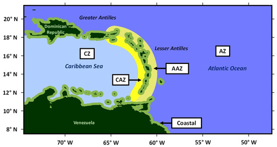
Figure 1.
Zones of the study area: Caribbean Zone (CZ), Atlantic Zone (AZ), Caribbean Antilles Zone (CAZ), Atlantic Antilles Zone (AAZ), and the coastal zone. Land areas are shown in dark green.
To better assess the effect of wind on the Sargassum strandings and distribution, the study area was divided into 5 zones. This division is motivated by differences in oceanic dynamics and the abundance of Sargassum in these zones (Figure 1):
- The coastal zone (Coastal) extends within 30 km from the coasts;
- The Atlantic Antilles Zone (AAZ) (Atlantic close-offshore area) is delimited by an outer arc 150 km east of the Antilles arc (encompassing but not including the coastal zone);
- The Atlantic Zone (AZ) (Atlantic far-offshore area) extends beyond the AAZ to the Atlantic Ocean;
- The Caribbean Antilles Zone (CAZ) (Caribbean close-offshore area) is delimited by an outer arc 150 km west of the Antilles arc (encompassing but not including the coastal zone);
- The Caribbean Zone (CZ) (Caribbean far-offshore area) extends beyond the CAZ to the Caribbean Sea.
The Sargassum found in the Caribbean Sea is mainly brought by the Atlantic currents passing through the Lesser Antilles Arc, including the North Equatorial Guinea eddies and the reverse front of the North Brazil Current [33,35,36,37,38]. The different zones allow the study of the spatial effects on the distribution of Sargassum.
2.2. Sargassum Dataset
The Sargassum data used in this study are derived from the OLCI satellite sensor. OLCI is an instrument on board the Sentinel-3A and Sentinel-3B satellites launched in 2016 and 2018, respectively, by the European Union’s Copernicus Earth Observation Programme. The satellite images obtained by both OLCI sensors have a spatial resolution of 300 m/pixel with a swath width of 1270 km. Each of the two Sentinel-3 satellites has a revisit period of 1 to 2 days. The combination of the two satellites provided almost complete coverage of the study area every day. Our study period covers 1249 days from 2019 to 2022. Each OLCI satellite image was processed using a deep learning model to detect pixels containing Sargassum, as described by Laval et al. [39]. The images obtained using this method contain binary information about whether a pixel contains Sargassum.
2.3. Atmospheric Data
2.3.1. Wind
The surface wind data used are from the ERA5 reanalysis dataset [40], namely the zonal and meridional components of the wind, u and v, at 10 m every hour with a spatial resolution of 1/4° (available at https://cds.climate.copernicus.eu/, accessed on 28 October 2024). The temporal variability of the wind speed is analyzed using a moving mean over the study area (Figure 1) and the study period from 2019 to 2022. The wind model grid was interpolated to the resolution of the OLCI images to be associated with the satellite image pixels.
2.3.2. Cloud Fraction
A cloud mask was created for each day from the same OLCI images used for Sargassum. The cloud mask was calculated using the 754 nm and 865 nm bands of OLCI from the method adapted from [41] for MODIS by Schamberger et al. [42]. The cloud fraction was calculated as the ratio of cloud pixels to the total number of pixels in each area, excluding land pixels, for each day over the entire period.
2.4. Sargassum and Water Fraction
The fraction of water in a given area is defined as the number of cloud-free water pixels out of the total number of pixels:
Water pixels include Sargassum and Sargassum-free pixels. The total number of pixels includes water and cloud pixels without land pixels.
The fraction of Sargassum pixels (or Sargassum fraction in short) in a given area is the number of pixels containing Sargassum over the total number of cloud-free water pixels:
The fractions vary between 0 and 1. The temporal variability of the Sargassum fraction is analyzed using a moving mean over 30 days (Figure 2).
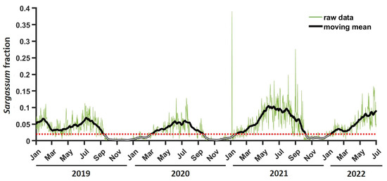
Figure 2.
Temporal variation in the Sargassum fraction (green line) and its moving mean (black line) in the whole study area between 2019 and 2022. Periods of low Sargassum fraction with a moving mean below 0.02 (dashed red horizontal line) are shown in gray.
2.5. Sargassum Aggregation Parameters
A Sargassum aggregation is an indivisible group of Sargassum rafts in satellite imagery [39]. Here, we define an aggregation as a set of pixels that share a common side or vertex between pixels or an isolated pixel (Figure 3). Around one million Sargassum aggregations were tagged between 2019 and 2022.
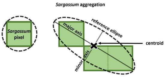
Figure 3.
Diagram of a Sargassum aggregation and the characteristics derived from its reference ellipse: major axis, minor axis, and center.
For each aggregation, geometric parameters were defined: area, length, width, and location of the aggregation. The area of an aggregation is defined as the number of pixels in the aggregation. The other geometric parameters are determined using a reference ellipse that represents the shape of the aggregation (Figure 3). The center of the reference ellipse is the centroid of the aggregation. The minor and major axes of the reference ellipse are such that the ellipse has the same second moment of area as the aggregation (hence not the same area). The aggregation geometric parameters are then defined as follows:
- The length corresponds to the major axis of the reference ellipse;
- The width corresponds to the minor axis of the reference ellipse, perpendicular to the major axis;
- The location is defined by the center of the reference ellipse by longitude and latitude. The location is used to assign Sargassum aggregations to zones and wind components.
The smallest reference ellipse, corresponding to a single-pixel aggregation, has a length and width of 1.15 pixels (i.e., a circle of 0.35 km diameter) with the same second moment of area of 1.35 × 10⁻³ km4 for both.
2.6. Representation of the Size of Sargassum Aggregations
We chose the area as a proxy for the size of the aggregations, while the length and width were used only to characterize the shape. As mentioned in Section 2.5, about 1 million aggregations were analyzed, with areas ranging from 1 pixel to many pixels. In the following, the aggregation surface area is studied as a continuous variable described by classes, [Ai, Ai+1[, whose limits are the successive terms of the geometric sequence with first member A0 and ratio 2. Then, the general term is
with n as the class range corresponding to the largest area found in the whole dataset. The possible smallest surface area, A0, is 1 pixel, i.e., A0 = 0.3 km × 0.3 km = 0.09 km2.
Ai = A0 2i; i = 1, …, n
The mode value was not estimated from the modal class but rather from the distribution’s probability density function to characterize the surface area distribution. This approach was chosen because it provides a more accurate representation of the mode, especially in skewed distributions where the modal class might not capture the peak accurately. The variation in the distribution at the left and right of the mode was characterized by two linear regressions on a logarithmic scale. Here, the logarithm used in these regressions is the decimal logarithm.
with p as the probability density, k as the slope in the logarithmic axis, and log10(a) as the intercept (the intersection value with the y-axis). Alternately, p can be expressed as a power law, p = a Ak. Although log10(a) and a appear in the equations, it is not explicitly used for interpretation in this article; we focus solely on the slope value.
log10(p) = k log10(A) + log10(a)
2.7. Dataset Selection
2.7.1. Image Selection Using Sargassum Fraction
For the analysis, we only included periods when Sargassum is consistently present in the study area to avoid seasonal bias. Periods with consistent Sargassum presence are defined as having the running mean of the Sargassum fraction being greater than 0.02. Figure 2 shows that the corresponding periods are from March to September, which includes the April to August period of the highest occurrence of Sargassum strandings in the study area according to local observations and as reported by [33], as well as January, February, and October, depending on the year. Furthermore, within the selected period, we discarded images with a Sargassum fraction lower than 0.01. Using these criteria, we retained about 68% of the initial images (i.e., 851 of 1249).
This selection, based on the Sargassum fraction, allowed us to limit the analysis to periods of effective presence of Sargassum in the study area, thus eliminating any wrong conclusions related to the wind effect on Sargassum presence.
2.7.2. Image Selection Using Cloud Fraction
Cloud fraction in the satellite images is another factor used to select our samples. Figure 4 shows the Sargassum fraction as a function of cloud cover. The median of the Sargassum fraction is constant, around 0.05, for a cloud fraction between 0 and 0.7. When the cloud fraction is greater than 0.7, the Sargassum fraction median decreases to reach half that value (0.025). This may indicate that the related images are not representative of calculating the Sargassum fraction, and this could introduce a bias. Because only a few images were concerned (7 images), they were removed. Therefore, our final sample is now composed of 844 images.
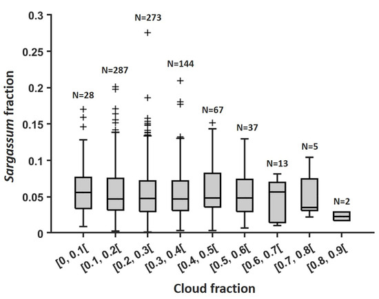
Figure 4.
Boxplot of Sargassum fraction as a function of cloud fraction. “+” indicates the outlier data not considered in the boxplot estimation.
2.7.3. Selection of Wind Speed Range
To define the range of wind speed available for analysis in the satellite dataset, we computed the distribution of images against wind speed (Figure 5). We defined 16 wind classes between 0 and 16 m·s−1, with a 1 m·s−1 range each. For each image and each wind class present in the image, the water and Sargassum fractions (Equations (1) and (2)) were calculated. Low water fractions and low Sargassum fractions (less than 0.05 and 0.001, respectively) were discarded, as they were not considered representative for this study. Based on those criteria, Figure 5 (dark bars) shows that only very few images (15 or less) contribute to wind classes outside to [2, 12[ m·s−1. Therefore, we only analyzed the classes between 2 and 12 m·s−1 in this study.
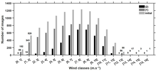
Figure 5.
The number of images for each wind class, for the different sampling of the satellite images: (1) sample outside the Sargassum period, high cloud fraction, and low Sargassum abundance; (2) after deletion of classes unrepresentative of water and Sargassum fraction.
To illustrate the impact of sample selection using the Sargassum fraction, cloud fraction, and water fraction on the wind classes, Figure 5 shows the samples available for each wind class before and after reducing the dataset.
3. Results
3.1. Temporal Variation in Wind, Cloud Fraction, and Sargassum Fraction
3.1.1. Wind Variability
Over the entire timeframe of the study and the entire study area, the winds varied between 0.002 and 20 m·s−1. The mean wind from the moving mean has similar variability between the Caribbean (CZ + CAZ) and Atlantic (AZ + AAZ) zones, as illustrated by Figure 6. We distinguish a period of high wind and a period of low wind, observed around the well-known dry and wet seasons of the region. The high wind season is slightly longer in the Caribbean zone (8 months, from January to August) than in the Atlantic zone (7 months, from January to July). Globally, winds are stronger in the Caribbean zone compared with the Atlantic zone (mean wind 8.5 m·s−1 and 7.5 m·s−1, respectively). Therefore, the weak wind season is shorter in the Caribbean zone (4 months, from September to December) than in the Atlantic zone (5 months, from August to December). Winds are weaker in the Atlantic zone, with a mean wind of 7.5 m·s−1 and 6.5 m·s−1 in the Caribbean zone. The minimum wind is 5.5 m·s−1 in September in the Caribbean zone, whereas it can reach a minimum of 4.5 m·s−1 in the Atlantic zone.
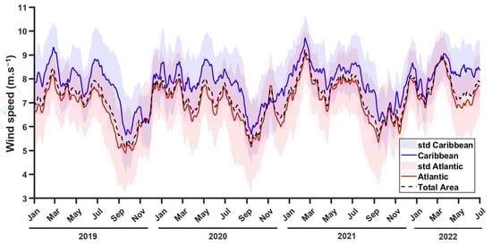
Figure 6.
Moving mean of wind speed from 2019 to 2022, outside the coastal zone, for the whole study area (dashed black line), the Caribbean zone (CZ + CAZ; solid blue line) with its standard deviation (solid blue zone), and the Atlantic zone (AZ + AAZ, solid red line) with its standard deviation (solid red zone).
3.1.2. Cloud Fraction Variability
Over the four years of the study, the distribution of cloud fraction within the same month is highly variable (Figure 7). April to June and August to November showed the highest medians, above 0.2, and the largest standard deviations. For these months, maxima above 0.6 of the cloud fraction are observed. For December to March and July, the median is most often below 0.2 of the cloud fraction. The standard deviation variation is smaller than for other months.
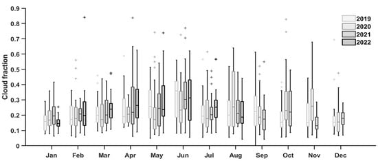
Figure 7.
Monthly distribution of cloud fraction for 2019, 2020, 2021, and 2022, illustrated by boxplot. “+” indicates the outlier data not considered in the boxplot estimation.
3.1.3. Sargassum Fraction Variability
First, in the study area, the Sargassum fraction in the total area increased from January to May, peaked in the May–July period (average Sargassum fraction between 0.06 and 0.12), and decreased from July to October (Figure 8; black curve). Between October and January, the average Sargassum fraction is the lowest, below 0.02, as illustrated in Figure 2 as well. The period of low Sargassum fraction decreased as time went on, from 6 months in 2019 to 3 months in 2021. Over the four years, a second peak occurring earlier in February was observed, usually much smaller (average fraction between 0.01 and 0.04) compared with the May–July peak, except in 2019, where the amplitudes of both peaks are similar (0.06 of the average fraction).
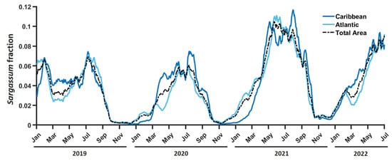
Figure 8.
Moving mean of Sargassum fraction from 2019 to 2022 for the entire study area (dashed black line), the Caribbean zone (CZ + CAZ; solid dark blue line), and the Atlantic zone (AZ + AAZ, solid light blue line).
The variation in the Sargassum fraction exhibited the same trend in the Caribbean (CZ + CAZ) and Atlantic (AZ + AAZ) zones. However, there is a time lag of about 1 month in the arrival of the Sargassum between the two zones, with an increase in the Sargassum fraction first seen in the Atlantic zone, then in the Caribbean zone. The Sargassum fraction is the highest in the Atlantic zone from January to March and in the Caribbean zone from March to October. The Sargassum season is longer in the Caribbean zone than in the Atlantic zone, lasting, respectively, from April to September and May to August.
The seasonal variation in Sargassum coverage usually observed in this zone, with a peak around June [2,31,33,43,44], is also observed in our data, with a slight shift between the tropical Atlantic zone and the Caribbean Sea (Figure 8). This shift is related to the connectivity between the two zones, Sargassum is transported from the Atlantic to the Caribbean through the Lesser Antilles Arc from spring to early fall by the Guiana Current, the North Brazil Current Rings, and the North Brazil Retroflection Current [33,35,37,43].
3.2. OLCI Sargassum Aggregations
3.2.1. Geometrical Characteristics of Sargassum Aggregations
In the area of interest from 2019 to 2022, during the Sargassum period, the Sargassum aggregation geometrical characteristics are distributed within a large range of values: areas ranging from 0.09 km2 to 32,000 km2, length from 0.35 km to 760 km, and width from 0.35 km to 290 km). Even though their distribution is extensive (Table 1), we observe the following:

Table 1.
Statistics on geometric characteristics of Sargassum aggregations (the ratio is not the ratio of medians of the length and width in the table but rather the median of the ratio W/L).
- A total of 25% of the aggregation areas are smaller than 1.1 km2, 50% are smaller than 4.7 km2, 75% are smaller than 18 km2, 90% are smaller than 53 km2, and 99% are smaller than 500 km2;
- A total of 25% of the aggregation lengths are smaller than 1.5 km, 50% are smaller than 3.4 km, and 90% are smaller than 17 km;
- A total of 25% of the aggregation widths are smaller than 1.1 km, 50% are smaller than 1.7 km, and 90% are smaller than 4.9 km.
One can notice that 50% of the aggregations have an area between 1.1 km2 and 18 km2 and 80% between 0.27 km2 and 53 km2.
Sargassum raft shapes have been described to range from circular to very elongated, or even in the form of filaments [24]. The ratio W/L is considered in the following to address the shapes of our aggregations. As illustrated in Figure 9, it decreases (i.e., the aggregations become more elongated) as the surface area increases. As illustrated in Table 1:
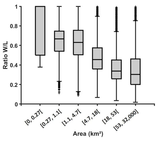
Figure 9.
Boxplot of the ratio W/L distribution as a function of the area classes corresponding to the distribution quantiles and deciles.
- The smallest 10% of aggregations (i.e., for A ≤ 0.27 km2) are mainly circular to slightly elongated: 0.50 ≤ W/L ≤ 1;
- The aggregations in the range 0.27 km2 ≤ A ≤ 4.7 km2 (i.e., 40%) are slightly elongated to elongated: 0.50 ≤ W/L ≤ 0.75);
- The aggregations in the range 4.7 km2 ≤ A ≤ 18 km2 (i.e., 25%) are elongated: 0.35 ≤ W/L ≤ 0.67; 25%;
- The largest 25% of aggregations (i.e., A ≥ 18 km2) are very elongated (0.20 ≤ W/L ≤ 0.45).
Aggregation surface areas smaller than 0.27 km2 (area of 3 pixels, about 10% of the sample), do have the most variable W/L ratio (0.5 ≤ W/L ≤ 1) (Figure 9). Three-pixel aggregations have a very limited spatial arrangement, ranging from circles to elongated ellipses. Single-pixel aggregations (6% of the sample) are circles, and two-pixel aggregations (3%) are elongated ellipses (W/L = 0.4 or W/L = 0.5).
It is important to keep in mind that the OLCI Sargassum aggregations are a set of Sargassum rafts (cf. Section 2.5). Sargassum rafts are smaller (typical area size is around ten square meters) [24,27] than the OLCI resolution (300 m × 300 m). Aggregation length and width, determined from the reference ellipse, are also longer than the raft dimensions. Besides, they are related to the aggregation surface area; for a given area by the OLCI pixels, the aggregation length and width can be determined using a second-order polynomial function that was the best fit of length and width as a function of area (Figure A1).
3.2.2. Area Distribution of Sargassum Aggregations
The probability density function of area classes follows the appearance of an asymmetric distribution with negative skewness (Pearson’s first skewness = −0.42), indicating that the mode is to the right of the mean. The modal class, i.e., the most represented area class of our dataset, is [6.76, 11.5[ km2 (Figure 10), and the mode from the density probability function is 7.5 km2, which is higher than the median (4.7 km2) and mean (4.3 km2).
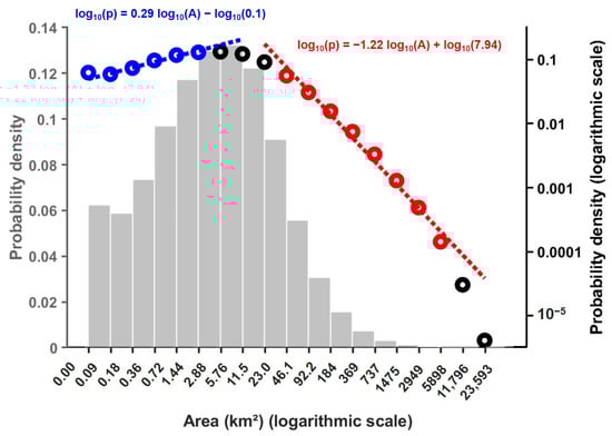
Figure 10.
Distribution of the area of Sargassum aggregations represented by (i) the histogram of the area classes (gray bars) and its probability density function (gray line), indicated by the left y-axis, and (ii) dots representing the distribution of the area classes on a logarithmic scale indicated in the right y-axis. The red and blue points correspond to those used to estimate the linear regressions, represented by the dashed red and blue lines, respectively.
The modal class divides the surface area dataset into two subsets (Figure 10): a subset on the left side of the mode (left subset) with small OLCI aggregations (area classes between 0 to 6 km2) and a subset on the right side of the mode (right subset) with large OLCI aggregations (area classes between 6 to 32,000 km2).
The first class, [0.09, 0.18[ km2, is a special class with more aggregations than the next (Figure 9 and Figure 10). In conjunction with the OLCI resolution, Sargassum aggregations smaller than 1 pixel (0.09 km2) are all classified in this first class.
Except for this first class, in the left subset, the number of aggregations per area class increases with size. The slope of the left logarithmic distribution (left slope) is around 0.29. On the other hand, the number of aggregations of the right subset decreases with size, and the slope of the right logarithmic distribution (right slope) is around −1.22. This slope is steeper than the slope on the left side.
3.2.3. Spatial Variation in Sargassum Aggregation Area Distribution
The size distribution of aggregations varies spatially. This is illustrated by the mode and the two slopes, presented in Figure 11. The major observations are as follows:
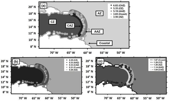
Figure 11.
Values of (a) the mode, (b) the left slope, and (c) the right slope of the surface area distribution as a function of the zones (Coastal, CZ, AZ, AAZ, and CAZ).
- Three different mode values can be observed. The CAZ mode is the highest (6.82 km2); it is a little bit lower than the global mode. CZ and AAZ are around 5 km2 (5.35 and 5.19 km2). The Coastal area and the AZ are the smallest, with a value of about 3.5 km2 (3.65 and 3.56 km2).
- The left slope is almost constant around 0.3 (between 0.31 and 0.35), except in the CZ zone, where it reduces to 0.26.
- The highest negative right slope is observed in the coastal zone (−1.67), and the lowest is in the CAZ zone (−1.04), followed by the AAZ zone (−1.14). The CZ and AZ zones have medium and quite similar slopes (−1.28 and −1.26 resp.).
3.3. Distribution of Sargassum Fraction and Aggregation Area as a Function of Wind Speed
3.3.1. Influence of Wind on Sargassum Fraction
The average Sargassum fraction decreases by 0.05 in each considered wind speed class (Figure 12). The same global tendency is observed for each month between January to September. The monthly averages for the Sargassum fraction from January to April and September are lower than the overall average for the Sargassum fraction, while they are higher for May to August. The maximum difference in the monthly Sargassum fraction is 0.06, observed between July and September. Consequently, the maximum estimated standard deviation is about 0.08, observed for weak wind speeds; the overall standard deviation envelope decreases and narrows as the wind increases.
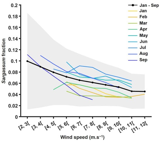
Figure 12.
Average Sargassum fraction in each wind class (black line) and per month from January to September (yellow to blue lines). The gray envelope represents the standard deviation of the average Sargassum fraction.
3.3.2. Influence of Wind on the Distribution of Sargassum Aggregations
The variation in the mode, the left slope, and the right slope increases with the wind speed until the wind speed reaches [8, 9[; [7, 8[ and [9, 10[ m·s−1, respectively (Figure 13). At these wind classes, the respective parameters reach their extremum and then decrease. The mode increases from 3.6 km2 to reach its maximum of 5 km2 in the wind class [8, 9[ m·s−1 and decreases until reaching the value of 4.1 km2 with a wind speed of [11, 12[ m·s−1. The right slope increases from 0.97 to reach its maximum of 1.3 in the wind class [9, 10[ m·s−1 and decreases until 1.02 for the maximum studied wind. On the other hand, the left slope is almost constant, with a slight increase from 0.26 to 0.31 reached in the [7, 8[ m·s−1 wind class, followed by a slightly stronger decrease to reach 0.23 at the maximum wind speed.
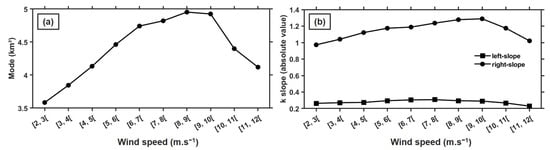
Figure 13.
Mode (a) and absolute value (b) of the left-slope (dots) and right-slope (squares) of the surface area distribution for each wind class.
Please note, for the right slope of the [9, 10[ m·s−1 wind class and above, the number of area classes available for the calculation of the linear regression gradually decreases from nine to five classes.
4. Discussion
4.1. Does the Cloud Fraction Bias Our Observations?
The presence of clouds in satellite imagery interferes with sea surface observations. It is conventional to say that cloud edges and shadows generally lead to false detections by index methods [34]. The method used in this paper, based on convolutional neural networks, avoids such difficulties by reducing the number of false detections [39]. Furthermore, the Sargassum fraction remains the same for all cloud coverages considered in this study (from 0 to 0.7), as illustrated in Figure 4.
The decrease observed between 2 and 12 m·s−1 wind speed (Section 3.3.1) occurs while the cloud fraction is quasi-constant (between 0.20 and 0.33), illustrating that the Sargassum fraction is less influenced by cloud fraction (which ranges from 0.20 to 0.33, Figure 14) than by wind speed. Then, around 13 m·s−1, while the cloud fraction is still 0.35, the Sargassum fraction is almost 0. Therefore, the wind effect seems predominant in the decrease in the Sargassum fraction.
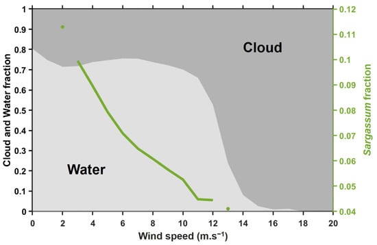
The lack of Sargassum pixels in the images for wind classes above 12 m·s−1 (Figure 5) could be associated with the lack or disappearance of Sargassum in the images during high wind events or the impossibility of detecting the presence of Sargassum by OLCI due to high wind speeds and wavy conditions. Furthermore, below 2 m·s−1, no data were considered because these wind speeds are mostly associated with the Sargassum low season (October to December), which is not part of our sample (Figure 6).
4.2. Disaggregation and Agglomeration of Sargassum Aggregations by Wind
Sargassum aggregations result either from the disaggregation of larger aggregations or from the agglomeration of smaller aggregations. On the one hand, the wind favors encounters between isolated Sargassum that can agglomerate. On the other hand, the wind induces water and atmospheric movements that can fragment existing Sargassum aggregations. The dominant effect depends on the size of aggregations and the wind speed. Large rafts of Sargassum are more likely to be observed when the sea is calm [22]. Sargassum rafts start to disaggregate with wind speed above 4 m·s−1, according to Woodcock et al. [26], or 5 m·s−1 according to Marmorino et al. [28].
Assuming a homogeneous disaggregation or agglomeration, the power law proposed for the area distribution of aggregations (Equation (4)) assumes that the frequency of the number of elements Fi+1 in area class Ai+1 (Equation (4)) can be expressed by the frequency of the number of elements Fi in the lower area class Ai. Then, from Equations (3) and (5), we can write
Fi+1 = 2k Fi
The slope k characterizes the disaggregation level (in absolute value) of the aggregation distribution. A distribution with a low level of segmentation is characterized by a large value of the left slope and a low absolute value of the right slope. When the distribution becomes more fragmented, the left slope decreases, while the right slope becomes steeper. At the same time, the mode shifts to the left, and the mean area value decreases.
For lower wind speeds (from 2 to 9 m·s−1), the mode shifts to the right as wind speed increases (Figure 13), both k-slopes increase, the size distribution tightens, and the number of both the smallest and largest aggregations decreases (Figure 15). This indicates that smaller aggregations in the left-subset agglomerate as the wind speed increases, whereas larger aggregations in the right-subset fragment. The first process populates area classes in the lower modal range, while the second process populates area classes in the upper modal range. This explains the higher occurrence of aggregations in the modal range of the size distribution due to the cumulative effect of agglomeration of smaller aggregations and disaggregation of larger ones.
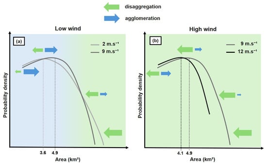
Figure 15.
Schematic representation of the evolution of the size distribution with wind, from a lower wind speed (black curve) to a higher wind speed (red curve) for (a) low to moderate wind conditions, from 2 to 9 m·s−1 and for (b) high wind conditions, from 9 to 12 m·s−1. The background colour indicates the dominant process: disaggregation (blue) or agglomeration (green).
For stronger wind (above 9 m·s−1), the mode shifts to the left as wind speed increases (Figure 13), and the left slope decreases, whereas the absolute value of the right slope increases, i.e., the overall distribution is shifted to the left, hence the number of largest aggregations decreases while the number of smaller aggregations increases (Figure 15). This confirms an overall disaggregation of the Sargassum aggregations in high wind conditions. Note that Figure 13 seems to indicate that the disaggregation process weakens above 10 m·s−1 as the absolute value of the k slope decreases. However, the calculation of k for the right subset is not reliable above 10 m·s−1 because the area classes corresponding to the largest aggregations are empty. The very fact that the largest aggregations disappear proves the disaggregation process; hence, the absolute value of the k slope should keep increasing as the wind speed increases.
In conclusion, in low to moderate wind conditions (from 2 to 9 m·s−1), wind increase favors the agglomeration of smaller Sargassum aggregations and the disaggregation of larger aggregations. In high wind conditions (above 9 m·s−1), wind increase favors the disaggregation of all aggregations.
4.3. Effect of Wind on the Decrease in Sargassum Fraction
In low to moderate wind conditions (from 2 to 9 m·s−1), the decrease in Sargassum fraction in satellite imagery as wind speed increases (Section 3.1.1.) can be explained by the agglomeration of small Sargassum aggregations inducing a decrease in the observed Sargassum surface.
In high wind conditions (above 9 m·s−1), the decrease in Sargassum fraction can be explained by the dispersal and disaggregation processes that may cause a gradual loss of Sargassum detection. Firstly, the smallest aggregations may become too small and too dispersed to be detected by OLCI due to their resolution [45]. Secondly, windy conditions induce waves that can submerge aggregations and make them undetectable in satellite imagery [24,26,46]. Finally, high wind conditions may induce Sargassum algal mortality, as wind stress can damage the aerocysts that keep Sargassum floating on the surface, causing them to sink and die [30].
4.4. Spatial Variability of Disaggregation and Agglomeration of Sargassum Aggregations
The rafts move mainly from the east (Atlantic) to the west (Caribbean). In the Lesser Antilles Arc, the funnel effect, in association with the topography and the eddies generated by return currents in the lee of the islands [47], creates biological accumulation zones [48,49] and favors the accumulation of aggregations. Hence, aggregations from the Atlantic offshore (AZ zone) become larger when they arrive in the Lesser Antilles Arc (AAZ and CAZ zones): the mode value increases with fewer smaller aggregations (left slope increase) and more larger aggregations (right slope increase). The phenomenon is more pronounced on the lee side (West side) of the Lesser Antilles islands (CAZ zone), where the mode value is the highest (6.82 km2), and the right slope is maximal as well (−1.04). This is confirmed by the observations of Ody et al. [24] and Goodwin et al. [27] during their at-sea campaign, where the largest rafts were found around the Caribbean coasts of the Lesser Antilles islands.
Once in the Caribbean offshore part (CZ zone), aggregations fall under similar conditions as the Atlantic offshore part (AZ zone), which are less favorable to agglomeration and where huge aggregations become rare (the absolute right-slope increases). However, aggregations remain larger in the Caribbean Sea than in the Atlantic (mode value of 5.35 km2 in CZ against 3.56 km2 in AZ; Figure 11a). This can be explained by the higher wind speed found in the Caribbean Sea than in the Atlantic Ocean (2 m·s−1 stronger; Figure 6); the aggregations would be more frequent in the high wind classes of the low wind regime (from 2 to 9 m·s−1; Figure 15), i.e., the size of the aggregations would increase towards the modal value.
The coastal zone has a different condition than the other zones, more impacted by disaggregation, consistent with the observations of sea users in Martinique who report that rafts are smaller near coasts.
5. Conclusions
This study analyzed four years of OLCI Sargassum imagery in the West Indies, beyond the seasonal and interannual variability described by several authors [2,43]. This study focused on the effect of wind speed on Sargassum spatial distribution and segmentation. The analysis emphasized the following findings:
- The Sargassum coverage decreases with wind speed and reaches zero when wind speed reaches 13 m·s−1. While agglomeration explains that tendency for lower wind speeds, the decrease in Sargassum fraction for higher wind speeds disaggregation indicates either a lesser detectability or a loss of Sargassum amount;
- The size distribution of Sargassum aggregations results from two opposite processes, mainly driven by wind: agglomeration and disaggregation;
- ○
- In low to moderate wind conditions (from 2 to 9 m·s−1), wind has a dual effect: it agglomerates smaller aggregations and disaggregates larger ones. In these wind regimes, the agglomeration process dominates, increasing the average size of aggregations;
- ○
- In higher wind conditions (above 9 m·s−1), disaggregation outweighs agglomeration, inducing a decrease in the average size of aggregations.
The size distribution varies spatially. On the one hand, it is influenced by the different wind regimes between the Caribbean and the Atlantic. In the Caribbean, winds are stronger in the low–moderate wind range (2 to 9 m·s−1) than in the Atlantic, which increases agglomeration. On the other hand, the topography between the Lesser Antilles Arc, the offshore areas, and the coastal areas also influences the size distribution. In contrast to offshore areas, the islands of the Lesser Antilles Arc are accumulation areas that favor agglomeration. In addition, coastal areas favor disaggregation due to wave and tidal dynamics, which intensify in coastal areas.
This study contributes to a better understanding of the dynamics of disaggregation and agglomeration of Sargassum rafts and the response of Sargassum spatial distribution to wind. Such knowledge is of interest to improve the modeling of Sargassum growth and transport and, ultimately, the prediction of Sargassum stranding events. Short-term and long-term predictions are key tools to help populations affected by Sargassum inundation, offering decision-makers and local authorities the possibility to adapt their prevention and mitigation strategies to the influx of Sargassum approaching the coast.
Author Contributions
Conceptualization, M.L., Y.A., J.D., L.C. and C.C.; methodology, M.L., L.C., J.D. and C.C.; software, J.D., L.C. and A.S.-G.; formal analysis, M.L., Y.A., J.D., L.C. and C.C.; resources, M.L., J.D. and L.C.; data curation, M.L., J.D. and C.C.; writing—original draft preparation, M.L., Y.A., J.D. and C.C.; writing—review and editing, Y.A., J.D., L.C., P.D.-N., A.C.d.S., P.Z., R.D. and C.C.; supervision, C.C.; funding acquisition, R.D. and P.Z. All authors have read and agreed to the published version of the manuscript.
Funding
This research was funded by the National Research Agency (ANR) in the SargAlert project (grant number: ANR-22-SARG-0001-01), FACEPE (grant number: APQ-0411-1.08/22) and by the Territorial Authority of Martinique (CTM; grant number: MQ0027405).
Data Availability Statement
The OLCI Sargassum data set used in this study will be made available through the web portal of the SargAlert Project at https://sargalert.lis-lab.fr (accessed on 25 October 2024). In the meantime, they are available on request from the corresponding author.
Acknowledgments
The authors would like to thank Copernicus Open Access Hub for providing Sentinel-3/OLCI data.
Conflicts of Interest
The authors declare no conflicts of interest.
Appendix A
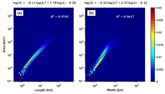
Figure A1.
Density plot of the area of Sargassum aggregations as a function of their length (a) and width (b), presented by the logarithmic scale axis. The color scale represents the probability density. Area, length, and width are from the entire dataset. The black line represents a second-order polynomial fitting the distribution of the Sargassum area as a function of their length (a) and (b) width (R2 = 0.97 and 0.96, respectively).
References
- Ardron, J.; Halpin, P.; Roberts, J.; Cleary, J.; Moffitt, R.; Donnelly, B. Where Is the Sargasso Sea? Sargasso Sea Alliance Science Report Series; Duke University Marine Geospatial Ecology Lab & Marine Conservation Institute: Beaufort, NC, USA, 2011; 24p. [Google Scholar]
- Wang, M.; Hu, C.; Barnes, B.B.; Mitchum, G.; Lapointe, B.; Montoya, J.P. The Great Atlantic Sargassum Belt. Science 2019, 365, 83–87. [Google Scholar] [CrossRef] [PubMed]
- de Széchy, M.T.M.; Guedes, P.M.; Baeta-Neves, M.H.; Oliveira, E.N. Verification of Sargassum natans (Linnaeus) Gaillon (Heterokontophyta: Phaeophyceae) from the Sargasso Sea off the Coast of Brazil, Western Atlantic Ocean. Check List 2012, 8, 638–641. [Google Scholar] [CrossRef]
- Gower, J.; Young, E.; King, S. Satellite Images Suggest a New Sargassum Source Region in 2011. Remote Sens. Lett. 2013, 4, 764–773. [Google Scholar] [CrossRef]
- Smetacek, V.; Zingone, A. Green and Golden Seaweed Tides on the Rise. Nature 2013, 504, 84–88. [Google Scholar] [CrossRef]
- Maréchal, J.-P.; Hellio, C.; Hu, C. A Simple, Fast, and Reliable Method to Predict Sargassum Washing Ashore in the Lesser Antilles. Remote Sens. Appl. Soc. Environ. 2017, 5, 54–63. [Google Scholar] [CrossRef]
- Trinanes, J.; Putman, N.F.; Goni, G.; Hu, C.; Wang, M. Monitoring Pelagic Sargassum Inundation Potential for Coastal Communities. J. Oper. Oceanogr. 2023, 16, 48–59. [Google Scholar] [CrossRef]
- Chávez, V.; Uribe-Martínez, A.; Cuevas, E.; Rodríguez-Martínez, R.E.; van Tussenbroek, B.I.; Francisco, V.; Estévez, M.; Celis, L.B.; Monroy-Velázquez, L.V.; Leal-Bautista, R.; et al. Massive Influx of Pelagic Sargassum spp. on the Coasts of the Mexican Caribbean 2014–2020: Challenges and Opportunities. Water 2020, 12, 2908. [Google Scholar] [CrossRef]
- Schling, M.; Guerrero Compeán, R.; Pazos, N.; Bailey, A.; Arkema, K.; Ruckelshaus, M. The Economic Impact of Sargassum: Evidence from the Mexican Coast; IDB Working Paper Series; Inter-American Development Bank (IDB): Washington, DC, USA, 2022. [Google Scholar] [CrossRef]
- van Tussenbroek, B.I.; Hernández Arana, H.A.; Rodríguez-Martínez, R.E.; Espinoza-Avalos, J.; Canizales-Flores, H.M.; González-Godoy, C.E.; Barba-Santos, M.G.; Vega-Zepeda, A.; Collado-Vides, L. Severe Impacts of Brown Tides Caused by Sargassum spp. on near-Shore Caribbean Seagrass Communities. Mar. Pollut. Bull. 2017, 122, 272–281. [Google Scholar] [CrossRef]
- Rodríguez-Martínez, R.E.; Medina-Valmaseda, A.E.; Blanchon, P.; Monroy-Velázquez, L.V.; Almazán-Becerril, A.; Delgado-Pech, B.; Vásquez-Yeomans, L.; Francisco, V.; García-Rivas, M.C. Faunal Mortality Associated with Massive Beaching and Decomposition of Pelagic Sargassum. Mar. Pollut. Bull. 2019, 146, 201–205. [Google Scholar] [CrossRef]
- Maurer, A.S.; Stapleton, S.P.; Layman, C.A.; Burford Reiskind, M.O. The Atlantic Sargassum Invasion Impedes Beach Access for Nesting Sea Turtles. Clim. Chang. Ecol. 2021, 2, 100034. [Google Scholar] [CrossRef]
- Maurer, A.S.; Gross, K.; Stapleton, S.P. Beached Sargassum Alters Sand Thermal Environments: Implications for Incubating Sea Turtle Eggs. J. Exp. Mar. Biol. Ecol. 2022, 546, 151650. [Google Scholar] [CrossRef]
- Resiere, D.; Valentino, R.; Nevière, R.; Banydeen, R.; Gueye, P.; Florentin, J.; Cabié, A.; Lebrun, T.; Mégarbane, B.; Guerrier, G.; et al. Sargassum Seaweed on Caribbean Islands: An International Public Health Concern. Lancet 2018, 392, 2691. [Google Scholar] [CrossRef] [PubMed]
- Resiere, D.; Mehdaoui, H.; Florentin, J.; Gueye, P.; Lebrun, T.; Blateau, A.; Viguier, J.; Valentino, R.; Brouste, Y.; Kallel, H.; et al. Sargassum Seaweed Health Menace in the Caribbean: Clinical Characteristics of a Population Exposed to Hydrogen Sulfide during the 2018 Massive Stranding. Clin. Toxicol. 2021, 59, 215–223. [Google Scholar] [CrossRef] [PubMed]
- de Lanlay, D.B.; Monthieux, A.; Banydeen, R.; Jean-Laurent, M.; Resiere, D.; Drame, M.; Neviere, R. Risk of Preeclampsia among Women Living in Coastal Areas Impacted by Sargassum Strandings on the French Caribbean Island of Martinique. Environ. Toxicol. Pharmacol. 2022, 94, 103894. [Google Scholar] [CrossRef]
- Liranzo-Gómez, R.E.; Gómez, A.M.; Gómez, B.; González-Hernández, Y.; Jauregui-Haza, U.J. Characterization of Sargassum Accumulated on Dominican Beaches in 2021: Analysis of Heavy, Alkaline and Alkaline-Earth Metals, Proteins and Fats. Mar. Pollut. Bull. 2023, 193, 115120. [Google Scholar] [CrossRef]
- Silva, T.M.; Waked, D.; Bastos, A.C.; Gomes, G.L.; Veras Closs, J.G.; Tonin, F.G.; Rossignolo, J.A.; Do Valle Marques, K.; Veras, M.M. A Custom, Low-Cost, Continuous Flow Chamber Built for Experimental Sargassum Seaweed Decomposition and Exposure of Small Rodents to Generated Gaseous Products. Heliyon 2023, 9, e18787. [Google Scholar] [CrossRef]
- Schell, J.M.; Goodwin, D.S.; Siuda, A.N.S. Recent Sargassum Inundation Events in the Caribbean: Shipboard Observations Reveal Dominance of a Previously Rare Form. Oceanography 2015, 28, 8–11. [Google Scholar] [CrossRef]
- Amaral-Zettler, L.A.; Dragone, N.B.; Schell, J.; Slikas, B.; Murphy, L.G.; Morrall, C.E.; Zettler, E.R. Comparative Mitochondrial and Chloroplast Genomics of a Genetically Distinct Form of Sargassum Contributing to Recent “Golden Tides” in the Western Atlantic. Ecol. Evol. 2017, 7, 516–525. [Google Scholar] [CrossRef]
- Dibner, S.; Martin, L.; Thibaut, T.; Aurelle, D.; Blanfuné, A.; Whittaker, K.; Cooney, L.; Schell, J.M.; Goodwin, D.S.; Siuda, A.N.S. Consistent Genetic Divergence Observed among Pelagic Sargassum Morphotypes in the Western North Atlantic. Mar. Ecol. 2022, 43, e12691. [Google Scholar] [CrossRef]
- Parr, A. Quantitative Observations on the Pelagic Sargassum Vegetation of the Western North Atlantic. With Preliminary Discussion of Morphology and Relationships. Bull. Bingham Oceanogr. Collect. 1939, 6, 7. [Google Scholar]
- Butler, J.N.; Stoner, A.W. Pelagic Sargassum: Has Its Biomass Changed in the Last 50 Years? Deep Sea Res. Part A Oceanogr. Res. Pap. 1984, 31, 1259–1264. [Google Scholar] [CrossRef]
- Ody, A.; Thibaut, T.; Berline, L.; Changeux, T.; André, J.-M.; Chevalier, C.; Blanfuné, A.; Blanchot, J.; Ruitton, S.; Stiger-Pouvreau, V.; et al. From In Situ to Satellite Observations of Pelagic Sargassum Distribution and Aggregation in the Tropical North Atlantic Ocean. PLoS ONE 2019, 14, e0222584. [Google Scholar] [CrossRef]
- Woodcock, A. Subsurface Pelagic Sargassum. J. Mar. Res. 1950, 9. Available online: https://elischolar.library.yale.edu/journal_of_marine_research/722 (accessed on 25 October 2024).
- Woodcock, A.H. Winds Subsurface Pelagic Sargassum and Langmuir Circulations. J. Exp. Mar. Biol. Ecol. 1993, 170, 117–125. [Google Scholar] [CrossRef]
- Goodwin, D.S.; Siuda, A.N.S.; Schell, J.M. In Situ Observation of Holopelagic Sargassum Distribution and Aggregation State across the Entire North Atlantic from 2011 to 2020. PeerJ 2022, 10, e14079. [Google Scholar] [CrossRef] [PubMed]
- Marmorino, G.O.; Miller, W.D.; Smith, G.B.; Bowles, J.H. Airborne Imagery of a Disintegrating Sargassum Drift Line. Deep Sea Res. Part I Oceanogr. Res. Pap. 2011, 58, 316–321. [Google Scholar] [CrossRef]
- Langmuir, I. Surface Motion of Water Induced by Wind. Science 1938, 87, 119–123. [Google Scholar] [CrossRef]
- Sosa-Gutierrez, R.; Jouanno, J.; Berline, L.; Descloitres, J.; Chevalier, C. Impact of Tropical Cyclones on Pelagic Sargassum. Geophys. Res. Lett. 2022, 49, e2021GL097484. [Google Scholar] [CrossRef]
- Sun, Y.; Wang, M.; Liu, M.; Li, Z.B.; Chen, Z.; Huang, B. Continuous Sargassum Monitoring across the Caribbean Sea and Central Atlantic Using Multi-Sensor Satellite Observations. Remote Sens. Environ. 2024, 309, 114223. [Google Scholar] [CrossRef]
- Berline, L.; Ody, A.; Jouanno, J.; Chevalier, C.; André, J.-M.; Thibaut, T.; Ménard, F. Hindcasting the 2017 Dispersal of Sargassum Algae in the Tropical North Atlantic. Mar. Pollut. Bull. 2020, 158, 111431. [Google Scholar] [CrossRef]
- Bernard, D.; Biabiany, E.; Cécé, R.; Chery, R.; Sekkat, N. Clustering Analysis of the Sargassum Transport Process: Application to Beaching Prediction in the Lesser Antilles. Ocean Sci. 2022, 18, 915–935. [Google Scholar] [CrossRef]
- Wang, M.; Hu, C. Mapping and Quantifying Sargassum Distribution and Coverage in the Central West Atlantic Using MODIS Observations. Remote Sens. Environ. 2016, 183, 350–367. [Google Scholar] [CrossRef]
- Putman, N.F.; Goni, G.J.; Gramer, L.J.; Hu, C.; Johns, E.M.; Trinanes, J.; Wang, M. Simulating Transport Pathways of Pelagic Sargassum from the Equatorial Atlantic into the Caribbean Sea. Prog. Oceanogr. 2018, 165, 205–214. [Google Scholar] [CrossRef]
- Franks, J.S.; Johnson, D.R.; Ko, D.S.; Sanchez-Rubio, G.; Hendon, J.R.; Lay, M. Unprecedented Influx of Pelagic Sargassum along Caribbean Island Coastlines during Summer 2011. In Proceedings of the 64th Gulf and Caribbean Fisheries Institute; Gulf and Caribbean Fisheries Institute: Puerto Morelos, Mexico, 2012; pp. 6–8. [Google Scholar]
- Franks, J.S.; Johnson, D.R.; Ko, D.S. Pelagic Sargassum in the Tropical North Atlantic. GCR 2016, 27, SC6–SC11. [Google Scholar] [CrossRef]
- Andrade-Canto, F.; Beron-Vera, F.J.; Goni, G.J.; Karrasch, D.; Olascoaga, M.J.; Triñanes, J. Carriers of Sargassum and Mechanism for Coastal Inundation in the Caribbean Sea. Phys. Fluids 2022, 34, 016602. [Google Scholar] [CrossRef]
- Laval, M.; Belmouhcine, A.; Courtrai, L.; Descloitres, J.; Salazar-Garibay, A.; Schamberger, L.; Minghelli, A.; Thibaut, T.; Dorville, R.; Mazoyer, C.; et al. Detection of Sargassum from Sentinel Satellite Sensors Using Deep Learning Approach. Remote Sens. 2023, 15, 1104. [Google Scholar] [CrossRef]
- Hersbach, H.; Bell, B.; Berrisford, P.; Biavati, G.; Horányi, A.; Muñoz Sabater, J.; Nicolas, J.; Peubey, C.; Radu, R.; Rozum, I.; et al. ERA5 Hourly Data on Single Levels from 1940 to Present. 2018. Available online: https://cds.climate.copernicus.eu/datasets/reanalysis-era5-single-levels?tab=overview (accessed on 25 October 2024).
- Nordkvist, K.; Loisel, H.; Gaurier, L.D. Cloud Masking of SeaWiFS Images over Coastal Waters Using Spectral Variability. Opt. Express OE 2009, 17, 12246–12258. [Google Scholar] [CrossRef]
- Schamberger, L.; Minghelli, A.; Chami, M.; Steinmetz, F. Improvement of Atmospheric Correction of Satellite Sentinel-3/OLCI Data for Oceanic Waters in Presence of Sargassum. Remote Sens. 2022, 14, 386. [Google Scholar] [CrossRef]
- Brooks, M.; Coles, V.; Hood, R.; Gower, J. Factors Controlling the Seasonal Distribution of Pelagic Sargassum. Mar. Ecol. Prog. Ser. 2018, 599, 1–18. [Google Scholar] [CrossRef]
- Jouanno, J.; Morvan, G.; Berline, L.; Benshila, R.; Aumont, O.; Sheinbaum, J.; Ménard, F. Skillful Seasonal Forecast of Sargassum Proliferation in the Tropical Atlantic. Geophys. Res. Lett. 2023, 50, e2023GL105545. [Google Scholar] [CrossRef]
- Putman, N.F.; Hu, C. Sinking Sargassum. Geophys. Res. Lett. 2022, 49, e2022GL100189. [Google Scholar] [CrossRef]
- Schamberger, L.; Minghelli, A.; Chami, M. Quantification of Underwater Sargassum Aggregations Based on a Semi-Analytical Approach Applied to Sentinel-3/OLCI (Copernicus) Data in the Tropical Atlantic Ocean. Remote Sens. 2022, 14, 5230. [Google Scholar] [CrossRef]
- De Falco, C.; Desbiolles, F.; Bracco, A.; Pasquero, C. Island Mass Effect: A Review of Oceanic Physical Processes. Front. Mar. Sci. 2022, 9. [Google Scholar] [CrossRef]
- Boehlert, G.W.; Watson, W.; Sun, L.C. Horizontal and Vertical Distributions of Larval Fishes around an Isolated Oceanic Island in the Tropical Pacific. Deep Sea Res. Part A Oceanogr. Res. Pap. 1992, 39, 439–466. [Google Scholar] [CrossRef]
- Wilson, B.; Hayek, L.-A.C. Islands, Currents, Eddies, Fronts… and Benthic Foraminifera: Controls on Neritic Distributions off Trinidad. Micropaleontology 2017, 63, 15–26. [Google Scholar] [CrossRef]
Disclaimer/Publisher’s Note: The statements, opinions and data contained in all publications are solely those of the individual author(s) and contributor(s) and not of MDPI and/or the editor(s). MDPI and/or the editor(s) disclaim responsibility for any injury to people or property resulting from any ideas, methods, instructions or products referred to in the content. |
© 2025 by the authors. Licensee MDPI, Basel, Switzerland. This article is an open access article distributed under the terms and conditions of the Creative Commons Attribution (CC BY) license (https://creativecommons.org/licenses/by/4.0/).