A Comparative Assessment of Reynolds Averaged Navier–Stokes and Large-Eddy Simulation Models: Choosing the Best for Pool-Type Fishway Flow Simulations

Abstract

Fishways are an important solution for mitigating the ecological impacts of river barriers, with their hydrodynamics playing a key role in their effectiveness. Computational fluid dynamics (CFD) is now one of the main tools to predict and characterize flow hydrodynamics, but choosing the most suitable turbulence model is considered one of its main challenges. Although substantial research has been carried out on vertical slot fishways, where the flow is predominantly two-dimensional, studies on pool-type fishways with bottom orifices remain scarce. In this study, three Reynolds averaged Navier–Stokes (RANS) turbulence models (the standard k-ε model, the renormalized group k-ε (RNG) model, and the standard k-ω model) and the large-eddy simulation (LES) model performances were compared to simulating the flow in a pool-type fishway with bottom orifices. ADV and PIV experimental data were used to assess model performance. While all the turbulence models accurately predicted the discharges and flow depths, the LES model outperformed the others in reproducing flow patterns, velocities, and turbulent kinetic energy. The RNG model also showed reasonable agreement with the experimental data. By contrast, the k-ε model delivered the poorest performance, failing to accurately predict the sizes of the recirculation zones and the locations of the recirculation axis and presenting the weakest agreement with the experimental observations. The value of the LES model in studying and characterizing fishway hydrodynamics, particularly concerning turbulence parameters, is highlighted.

1. Introduction

The fragmentation and regulation of rivers by human-made barriers such as dams and weirs have recently been highlighted as major threats to aquatic life sustainability, especially fish populations [1,2]. Fishways are one of the main solutions for mitigating the ecological impact of anthropogenic barriers while preserving their essential functions. They restore, at least partially, longitudinal connectivity, enabling fish to move past these obstacles [3]. Pool-type fishways are a technical type of fishway that consist of a series of pools, arranged in a stepped pattern and separated by cross-walls, which include features such as vertical slots, bottom orifices, and/or surface notches to facilitate fish movement from one pool to the next [4]. Fish passage performance is heavily influenced by hydrodynamic factors, with velocity and turbulence playing key roles [5,6,7,8]. In pool-type fishways with bottom orifices, water flows from one pool to the next through a series of orifices, generating high turbulence within each pool. The jets flowing from one pool to the next create recirculation zones and smaller swirling areas; strong velocity gradients at the jet edges, coupled with the recirculation zones, result in regions of shear and eddy formation. Energy dissipates in these regions, as well as through jet mixing within the pools [9]. This dynamic creates a highly complex flow field that is challenging to predict and accurately characterize.

Computational fluid dynamics (CFD) studies have increased notably in recent years due to their versatility and accuracy and also due to advances in computer technology [10]. CFD has become a major tool for studying complex flow physics [6,11,12,13,14,15,16,17,18,19,20,21] and is widely used to predict and characterize flow hydrodynamics, improving the design of hydraulic structures while reducing or even eliminating the need for physical models, thereby saving time and cutting costs. Turbulence plays a critical role in most hydraulic engineering problems, including fishway performance [22,23,24,25], as it significantly affects drag, separation, swirling, recirculation, vorticity distribution, and energy dissipation.

Turbulent flows are characterized by fluctuating velocity fields and unsteady vortices emerging at various length scales that interact with each other. Since these fluctuations can occur at small scales and high frequencies, directly simulating them is computationally prohibitive for many engineering applications [10]. Direct numerical simulations (DNSs) solve the original Navier–Stokes equations without any model assumptions, resolving all scales of turbulent motion. While DNS is an invaluable tool for fundamental turbulence research, the computational resources and simulation time required for practical applications at larger Reynolds numbers remain prohibitive [10,26].

Reynolds averaging and filtering are alternative methods to transform the Navier–Stokes equations, focusing on the large-scale and non-fluctuating features of the flow. These methods eliminate the need to directly simulate small-scale turbulent fluctuations. However, the effects of the small scales and fluctuating components must be modelled to fully characterize the flow [10,27].

The Reynolds averaging approach decomposes turbulence into its mean and fluctuating components, introducing an additional term in the Navier–Stokes equations: the Reynolds stress tensor. A turbulence model is required to compute the Reynolds stresses. Models such as the standard k-ε model, the renormalized group k-ε (RNG) model, and the standard k-ω model have been extensively applied [8,10,20,28,29,30,31]. These models rely on the Boussinesq assumption, which relates apparent turbulent shearing stresses to the mean strain through an apparent scalar turbulent or “eddy” viscosity [28].

The standard k-ε model is known to work well for simple flow scenarios, but its adequacy for complex recirculating or swirling flows, involving streamlined curvature and rotation, has been questioned [10,32].

The RNG model, a more recent approach, uses similar equations to the standard k-ε model [33,34] but derives its empirical constants explicitly, resulting in broader applicability [10,35]. The RNG model is generally more accurate than the standard k-ε model for flows involving rotation, boundary layers under strong adverse pressure gradients, separation, and recirculation [10,36].

The standard k-ω model, based on the Wilcox k-ω model, incorporates modifications to account for low Reynolds number effects, compressibility, and shear flow spreading. The k-ω model often outperforms the standard k-ε model and the RNG model for flows with streamwise pressure gradients, such as jets, wakes, and near-wall boundaries [10,35].

In large-eddy simulation (LES), the computational cost of direct simulation is reduced by filtering out the small-scale eddies (smallest length scales) through low-pass filtering of the Navier–Stokes equations. The largest and most energetic structures (large eddies) are computed directly, whereas the small-scale motions (sub-grid scale, SGS) are modelled. An advantage of LES over the Reynolds averaged Navier–Stokes (RANS) models is that LES directly captures the large eddies, which contain most of the turbulent energy and are primarily responsible for momentum transfer and turbulent mixing, in full detail. Although LES is more computationally demanding than the RANS approaches, it has become one of the most promising and successful tools for studying turbulent flows [37,38].

Despite its advantages, no universal model exists, as none can claim to be applicable to all turbulent flows [28]. Given this, having a diverse set of approaches to study turbulent flows is essential [39].

The use of CFD in fishway research has grown significantly, with an increasing number of studies published over the past 7–8 years [26]. However, due to the absence of a widely accepted standard procedure for simulating flow within fishways with CFD, the modelling equations, assumptions, and approximations must be tailored to the specific layout of the fishway being analyzed. Each study relies heavily on the expertise of the software user to make these decisions [26,40]. Selecting the most suitable turbulence model for a specific configuration remains one of the main challenges in numerical modelling [41,42].

RANS turbulence modelling has been the most widely used approach, appearing in over 65% of the studies, while LES turbulence modelling accounted for only 21% of the studies conducted so far [26]. Nonetheless, RANS turbulence models are generally regarded as less effective for evaluating turbulent parameters, which limits their accuracy in assessing fishway flow dynamics [42,43].

The majority of the studies to date have focused on vertical slot fishways (VSFs), accounting for over 50% of the total [26]. Among the studies using CFD for pool-type fishways with weirs and/or orifices (representing 15% of the total number of studies), nearly all applied RANS turbulence models, with the standard k-ε model being the most prevalent approach. Duguay et al. [42] used the standard k-ε model to compare the performance of OpenFOAM and FLOW-3D^® in simulating a pool-type fishway with alternating side surface notches. Similarly, Abeyratne et al. [44] applied the standard k-ε model to investigate flow dynamics in a pool-type fishway with weirs and orifices to optimize its design. Li et al. [45,46] also used the standard k-ε model to enhance the hydrodynamics of pool-type fishways, focusing on V-shaped and labyrinth weir configurations to improve fishway design. Likewise, Bravo-Córdoba et al. [47] used the standard k-ε model to characterize the hydrodynamics of a pool-type fishway with weirs. Ye et al. [48] used the same model to examine the flow hydrodynamics of a pool-type fishway with weirs and orifices, linking hydrodynamic parameters to eel swimming trajectories.

On the other hand, Abad et al. [49] analyzed the hydrodynamics of a Dutch pool and orifice fishway using the FLOW-3D^® RNG model. Wang et al. [50] also employed the RNG model to investigate the hydrodynamics of three types of pool-type fishways: VSFs, overflow weirs, and orifice pool-type fishways. Quaresma and Pinheiro [51] assessed the FLOW-3D^® LES model performance in accurately reproducing the flow hydrodynamics of pool-type fishways with bottom orifices.

Presently, selecting an appropriate turbulence model for 3D simulations of pool-type fishways with bottom orifices is a critical challenge in assessing their hydrodynamics. The choice directly impacts the accuracy of the predicted flow patterns, velocity distributions, and turbulence characteristics. While extensive research has been conducted devoted to modelling VSFs (as highlighted in a recent review by Tarena et al. [26]), where the flow is predominantly two-dimensional [51,52] modelling pool-type fishways with bottom orifices remains less understood. This knowledge gap is crucial, because as reported by Quaresma & Pinheiro [51], these structures induce highly three-dimensional flow patterns, creating complex recirculation zones and turbulence phenomenas. This is unlike VSFs, where vertical velocities are generally negligible except near the slot, especially under low slopes [24,53].These features pose a significant challenge for accurate model prediction due to high-velocity gradients and elevated vorticity, demanding advanced numerical modelling approaches [44,51,54]. Despite the growing use of CFD in fishway studies, to our knowledge, a direct comparative assessment of RANS models (the standard k-ε model, the RNG model, and the standard k-ω model) and the LES model for this fishway typology remains largely unexplored. This study aims to address this gap by identifying the most suitable turbulence model for analyzing pool-type fishways with bottom orifices, ultimately enhancing the accuracy and reliability of CFD models in fish passage engineering.

2. Materials and Methods

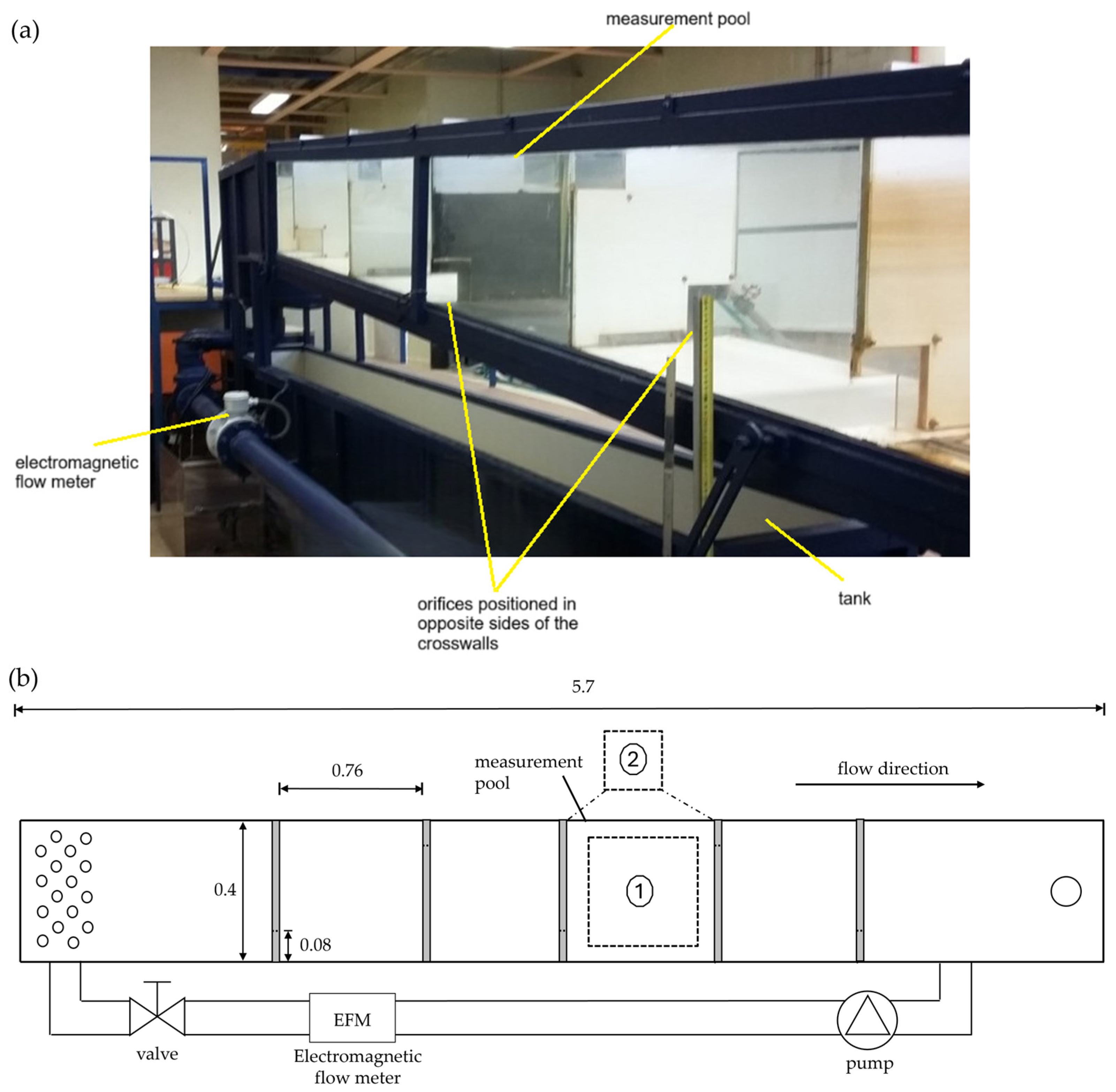
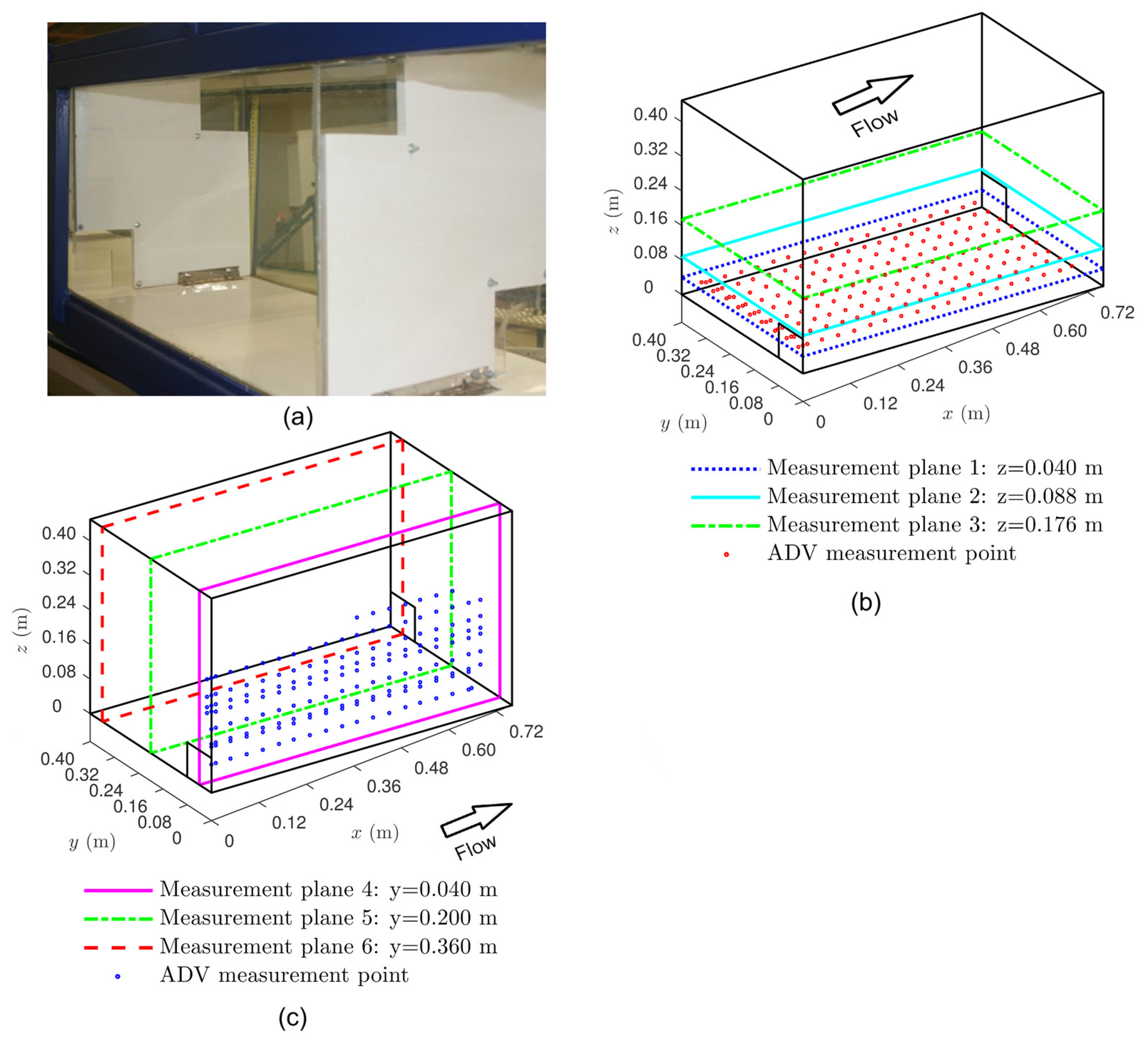
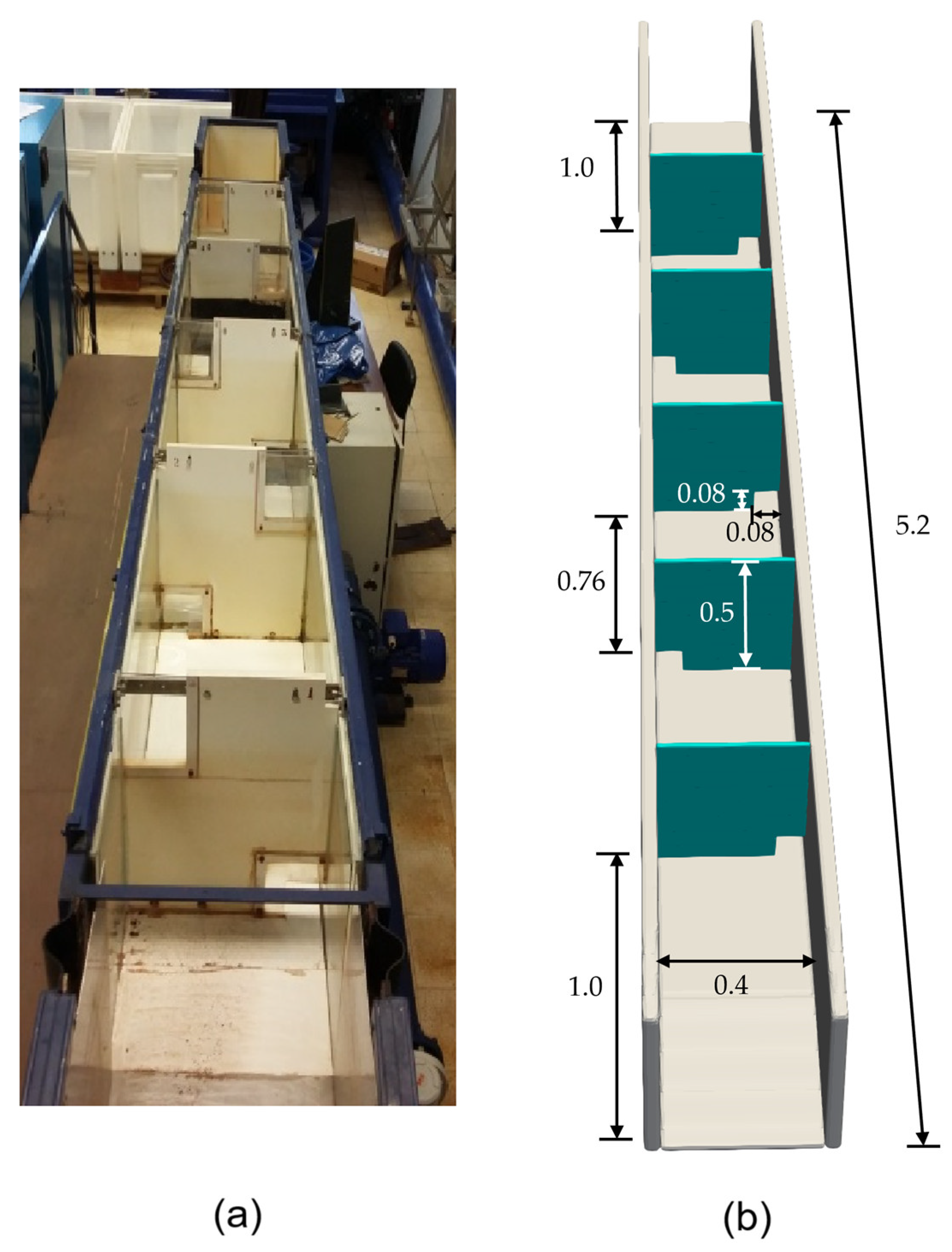
2.1. Experimental Procedure

A pool-type fishway facility installed at the Laboratory of Hydraulics and Environment of Instituto Superior Técnico (IST) was used for this study. This setup, a 1:2.5 scale model of the pool-type fishway used by Silva et al. [5], consists of a flume that is 5.7 m long, 0.4 m wide and 0.5 m high. It features glass sidewalls, an adjustable slope, and a recirculation circuit (Figure 1). The flume includes four pools, each measuring 0.76 m in length and 0.40 m in width, separated by five PVC cross-walls with square bottom orifices measuring 0.08 m × 0.08 m. Alternating orifices were positioned on opposite sides of the cross-walls (Figure 1), creating a sinusoidal flow path. The flume slope was set at 8.5%, and flow discharge was regulated by a pump frequency converter and measured with an electromagnetic flow meter (ABB WaterMaster FEV121, DN100, PN16, Lisboa, Portugal) installed in the recirculation pipe. A sluice valve controlled the downstream flow depth. Discharge was maintained at 4.4 ± 0.4% ls⁻¹, the head drop between pools (Δh) was 0.064 ± 5% m, and the mean water depth in each pool (h_m) was 0.352 ± 0.5% m.

3D instantaneous velocity measurements were performed with acoustic Doppler velocimetry (ADV, Nortek Group, Oslo, Norway), and two-dimensional instantaneous velocity maps were obtained with a particle image velocimetry system (PIV, Dantec Dynamics, Skovlunde, Denmark) (not simultaneously). Velocity measurements were conducted in the third upstream pool (Figure 2a) in six planes: three parallel to the flume bed (Figure 2b) at 0.04 m (half the height of the orifice), 0.088 m (25%h_m), and 0.176 m (50%h_m) high, and three vertical planes parallel to the sidewalls (Figure 2c) at the mid-width of the pool and of each orifice. The coordinate system used in this study was defined with its origin at the bottom-right corner of the third pool upstream orifice. The x-axis ran longitudinally, parallel to both the bottom and the flume axis; the y-axis was transverse; and the z-axis was perpendicular to the bottom. The instantaneous velocity components u, v, and w corresponded to the x-, y-, and z-axes, respectively. A detailed description of the experimental methodology, the reliability verification, and the uncertainty analysis of the experimental measurements can be found in Quaresma et al. [55]. The good agreement shown by Quaresma et al. [55] between PIV and ADV measurements guaranteed the ability of the performed experimental measurements to accurately represent the flow field and thus be used for the numerical model validation and turbulence model comparison.

2.2. CFD Model

The numerical modelling of the pool-type fishway flow field was performed using FLOW-3D^® (Version 11.2; 2016; https://www.flow3d.com accessed on 1 June 2016; Flow Science, Inc., Santa Fe, New Mexico, USA), a versatile commercial CFD software that solves the governing equations of fluid motion to generate transient, three-dimensional solutions. FLOW-3D^® has seen extensive application in hydraulic engineering [11,56,57,58,59]. In recent years, it has also been widely used in fishway research [26,42,60,61,62,63,64].

FLOW-3D^® employs finite volume and finite difference methods to solve the equations of fluid motion on a Cartesian staggered grid. A key feature of FLOW-3D^® is the Fractional Area/Volume Obstacle Representation (FAVOR^TM) method [65], which represents obstacles using fractional areas and volumes within a fixed orthogonal grid. Obstacles are modelled as zero-volume porosity regions, with the six components of wall shear stress incorporated implicitly in the equations to prevent numerical instabilities.

The volume of fluid (VOF) method was applied [66] to accurately capture free surface hydrodynamics. VOF includes three main components: defining the volume of fluid function (F-function), which represents the fraction of fluid in each cell (ranging from zero (no fluid) to one (fully filled with fluid)); solving the VOF transport equation; and setting the boundary conditions at the free surface. The free surface is identified by intermediate values of the fluid fraction within the cells. To solve the VOF transport equation, a suitable advection method was applied to minimize numerical diffusion of the free surface.

The computational domain can consist of either single-block or multi-block grids. The multi-block approach allows mesh refinement in specific areas, reducing memory usage and computational cost. Physical quantities are calculated independently within each grid block and exchanged between them. Pressures and velocities are linearly interpolated, whereas fluid fraction, thermal energy, scalars, and turbulent parameters are “overlaid” [67].

FLOW-3D^® offers six turbulence models: the Prandtl mixing length model, the one-equation model, the two-equation k-ε model, the renormalization group theory-based k-ε (RNG) model, the k-ω model, and the large-eddy simulation (LES) model. This study compares the performance of the four latter models. These turbulence models were chosen based on their frequency of use within the study domain and related fields, their availability, and their potential suitability for the specific type of flow being investigated.

Additional details about the theoretical and numerical foundations of FLOW-3D^® can be found in [35].

2.2.1. Model Geometry, Computational Domain, Grid, and Boundary Conditions

The entire fishway geometry (Figure 3a) was created in AutoCAD 2013 based on the dimensions of the physical model and imported into the software as a stereolithography (STL) file. The computational domain (Figure 3b) was then discretized using multi-block grids to effectively optimize the mesh with the physical model geometry, with each grid block created with a uniform cell size. Two mesh configurations were tested to ensure a mesh-independent solution.

The coarsest mesh setup used five grid blocks: one block encompassing the full fishway geometry and four nested blocks with half the cell size of the main block. The pool where velocity measurements were taken was contained within one of the nested blocks, while the other three covered the cross-walls of the additional pools. This configuration totalled 380,650 cells, with a main block cell size of 0.02 m (254 × 23 × 25 cells) and 0.01 m in the nested blocks (one block with 84 × 46 × 50 cells and three blocks with 6 × 46 × 50 cells).

A finer mesh configuration consisted of two grid blocks with a combined total of 2,714,000 cells. In this configuration, the main block had a uniform cell size of 0.01 m (508 × 46 × 50 cells), while the nested block containing the third pool had a cell size of 0.005 m (168 × 92 × 100 cells).

Pressure boundary conditions were defined for both the upstream and downstream boundaries based on experimentally observed water depths. The sidewalls and the bottom were modelled as no-slip boundaries, whereas a symmetry boundary condition was applied at the top, imposing zero normal velocity and zero gradients for other variables. The initial pressure was set to the atmospheric pressure. Gravity was applied in the negative z-direction and the positive x-direction so that the x-axis was parallel to the fishway bed.

2.2.2. Numerical Solver Options

The generalized minimum residual (GMRES) implicit solver was used in this study [68]. As the default solver in FLOW-3D^®, GMRES is a nonstationary iterative method with iteration-dependent coefficients [69] and is well-regarded for its accuracy and efficiency across a broad range of problems [35].

This study examined the effects of the following variables on the solution: (i) momentum advection method, with both first-order and second-order monotonicity-preserving options; (ii) turbulence model choice, including k-ε, RNG, k-ω, and LES models; (iii) surface roughness; and (iv) grid cell size dependency.

The impact of roughness was assessed by testing a range of Manning surface roughness coefficients, n, representative of the experimental facility, with a selected value of n = 0.01 m^−1/3s. In FLOW-3D^®, wall roughness was set using the roughness height, which was computed from the empirical Strickler formula [70] for the chosen n value. Since turbulence model selection is the primary focus, results are only shown for this roughness value. Similarly, only results using the second-order monotonicity-preserving advection method are presented, as this method yielded the best alignment with the experimental data.

To assess the uncertainty due to discretization in the numerical simulation results, a mesh sensitivity analysis was performed based on the ASME criteria [71]. Additionally, the LES_IQ_k verification index proposed by Celik et al. [72] was used to assess the LES models’ quality. A detailed investigation of the mesh sensitivity analysis of the LES turbulence model can be found in Quaresma et al. [51], where the numerical model results for four grid sizes were analyzed. Moreover, the mesh sizes considered were smaller or of similar size to previous pool-type fishway studies that used CFD to analyze pool-type fishway flows [43,73,74,75,76,77]. Predictions of mean-flow and turbulence quantities showed minimal differences between fine and coarse grid simulations for both RANS and LES models, so only coarse grid results are reported here. Simulations were run for enough time steps to reach steady-state conditions, confirm flow field steadiness, and obtain converged time-averaged values.

No further mesh refinement was conducted due to the satisfactory results achieved and the considerable increase in computational cost it would entail. Using the same mesh for all simulations with different turbulence models allowed for a consistent basis of comparison without mesh density influencing the evaluation of turbulence model performance.

3. Results

The three distinct RANS models and the LES model were compared concerning their effectiveness in reproducing key flow characteristics. The numerical results were also compared to the laboratory measurements from Quaresma et al. [55] to assess the predictive capabilities of both the RANS and LES models. For the LES model results, time-averaged velocities and turbulence statistics were determined through a time-averaging (Reynolds-averaging) approach.

3.1. Discharges and Flow Depths

Table 1. Comparison of measured and simulated discharges and flow depths.

Source	Measurement	Numerical Model
Turbulence Model	-	k-ε	RNG	k-ω	LES
Discharge (ls−1)	4.4	4.6	4.6	4.6	4.6
Relative difference (%)	-	4.6	4.7	4.6	4.8
Flow depth (m) 1	0.352	0.364	0.363	0.364	0.363
Average relative difference (%) 1	-	3.6	3.5	3.7	3.5

Notes: ¹ The flow depth and its average relative difference represent the averages across sixteen measured/computed points within the four pools. Relative differences were calculated by dividing the difference between the numerical and measured values by the measured values. 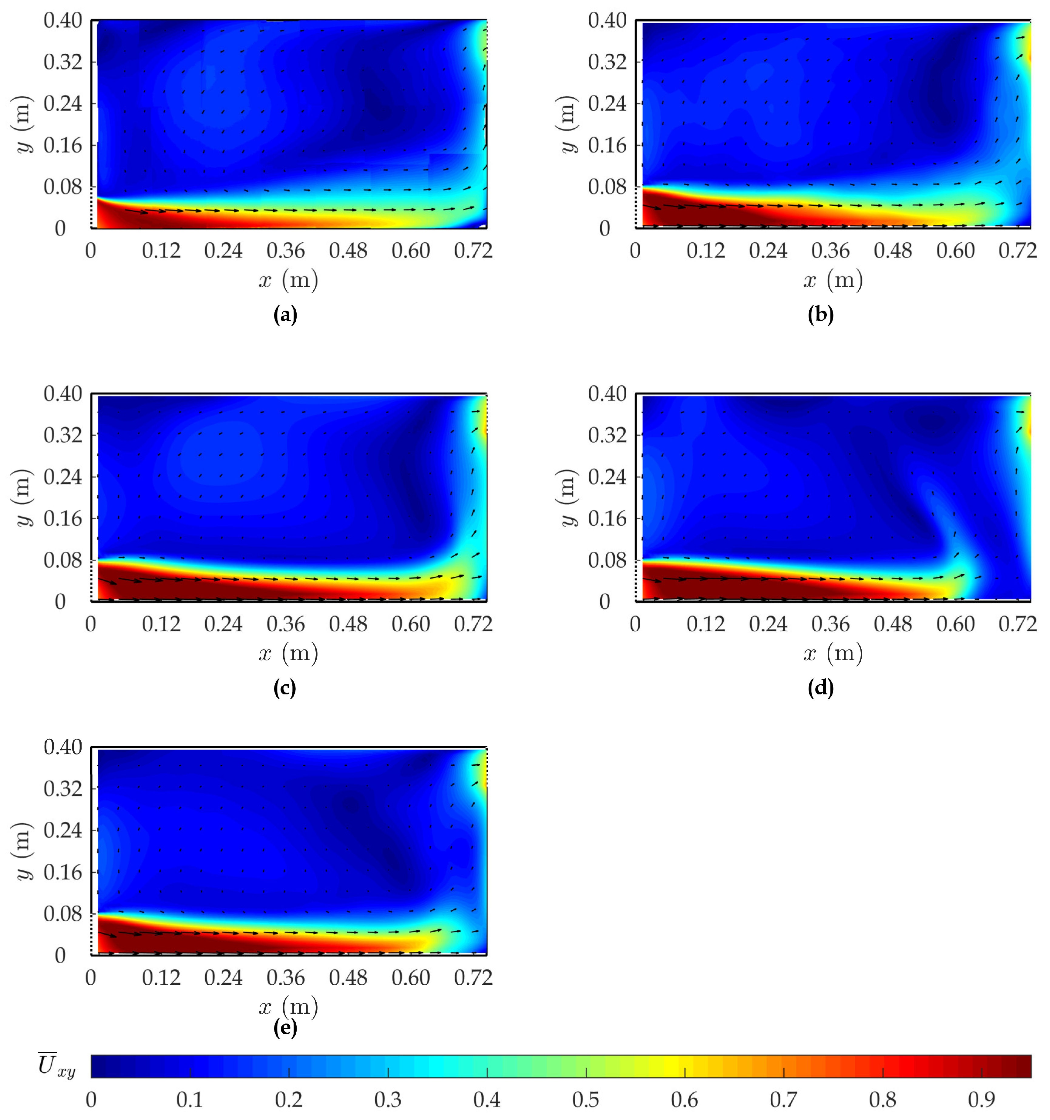LES: large-eddy simulation; k-ε, RNG (renormalized group k-ε), and k-ω models: RANS (Reynolds averaged Navier–Stokes) turbulence models.

shows the measured and predicted discharges, the average flow depths, and the relative differences. For flow depth, the reported relative difference is the average across the sixteen comparison points.

The results in Table 1 indicate that all turbulence models accurately predicted the discharges and flow depths. The difference between the numerical models’ discharges and the experimental discharge was 0.2 ls⁻¹, less than 5% for all turbulence models (ranging from 4.6% for the k-ε and k-ω models to 4.8% for the LES model). Concerning the flow depths, the differences ranged from 0.011 m for the RNG and LES models to 0.012 m for the k-ε and k-ω models (less than 4% for all turbulence models). The relative differences ranged from 3.5% for the RNG and LES models to 3.7% for the k-ω model. Thus, no notable differences were observed between the turbulence models for these hydrodynamic parameters.

3.2. Flow Patterns

Figure 4 compares time-averaged 2D streamline patterns in a plane parallel to the flume bed (plane 2—z = 25% h_m) and in a vertical plane (plane 5—mid-width of the pool), obtained from the PIV data, with those predicted by the turbulence models. The LES model stood out as the most accurate, closely capturing the experimental flow patterns.

The RNG model also performed well, though with minor deviations: in plane 2, the recirculation zone axis was slightly shifted towards the left sidewall and downstream cross-wall, and in plane 5, the main clockwise recirculation zone appeared wider while the counterclockwise zone near the downstream cross-wall was narrower than that observed in the experiments.

For the k-ε and k-ω models, recirculation eddies developed farther from the experimental source points. The discrepancies in the k-ε model were more pronounced where the recirculation zone axis in plane 2 was positioned significantly closer to the left sidewall and downstream cross-wall than in the experiments. In plane 5, both the k-ε and k-ω models showed a narrower main swirl zone, with secondary swirls appearing wider compared to the experimental data.

3.3. Velocities

Figure 5 presents the time-averaged 2D mean velocity magnitude and vector fields in plane 1 (half the height of the orifice), obtained from the PIV data, and the applied turbulence models. The LES model demonstrated the closest alignment with the experimental data. For this turbulent model, although the jet was slightly larger immediately downstream of the pool entrance, its development was similar to the experimental data jet development. The RNG model also provided a reasonable prediction of the mean velocity magnitude and direction, although the jet was larger, extended slightly farther downstream, and appeared narrower in the downstream region compared to the experimental results. The k-ε model showed the least agreement with the experimental data, with a smaller jet development compared to the experimental data. In all the turbulence models, the jet was slightly larger, particularly immediately downstream of the pool entrance. The highest difference in the time-averaged 2D velocity magnitude in this zone was 0.04 ms⁻¹, a relative difference of 4%.

To quantitatively assess the performance of the different turbulence models, statistical parameters were calculated to compare the numerical simulations results with the experimental measurements. The numerical simulations results obtained for the ADV measurement grid points were directly compared with the corresponding ADV data. Due to the higher spatial resolution of the PIV measurements relative to the numerical mesh size, the PIV data were interpolated within the mesh cells to facilitate comparison with the model results.

Table 2. Comparison of measured and simulated time-averaged velocity magnitudes: statistical model performance indicators for the different turbulence models.

		$\overline{\mathit{u}}$			$\overline{\mathit{v}}$			$\overline{\mathit{w}}$			$\overline{\mathit{U}}$
		MAD (ms−1)	R2	dr	MAD (ms−1)	R2	dr	MAD (ms−1)	R2	dr	MAD (ms−1)	R2	dr
CFD vs. ADV 1	k-ε	0.060	0.82	0.75	0.030	0.76	0.75	0.037	0.54	0.63	0.061	0.66	0.60
	RNG	0.037	0.91	0.85	0.019	0.90	0.84	0.025	0.77	0.75	0.040	0.82	0.73
	k-ω	0.039	0.92	0.84	0.018	0.92	0.85	0.027	0.75	0.73	0.037	0.83	0.75
	LES	0.031	0.93	0.87	0.020	0.90	0.83	0.026	0.78	0.73	0.032	0.85	0.79
CFD vs. PIV 2	k-ε	0.069	0.80	0.78	0.032	0.76	0.75	0.042	0.45	0.63	3
	RNG	0.040	0.92	0.87	0.021	0.90	0.83	0.028	0.72	0.75
	k-ω	0.047	0.92	0.85	0.021	0.89	0.83	0.031	0.68	0.72
	LES	0.038	0.92	0.88	0.023	0.90	0.82	0.035	0.73	0.69

Notes: ¹ All 840 measured points were included in the comparison. ² A total of 15,884 points were compared for the $\overline{u}$ time-averaged velocity component, 8963 for $\overline{v}$, and 6921 for $\overline{w}$. ³ Since the PIV measurements were performed with a 2D PIV system, the data could not be computed. $\overline{u}$, $\overline{v}$ and $\overline{w}$: time-averaged velocity components; $\overline{U}$: time-averaged velocity magnitude; R²: coefficient of determination; d_r: refined index of agreement; MAD: mean absolute difference $={\displaystyle \frac{1}{N}}{\sum }_{i=1}^N\left|a_{experimental}-a_{numerical}\right|.$

displays the mean absolute differences (MADs), coefficients of determination (R²), and refined indexes of agreement (d_r) for the time-averaged velocity components ($\overline{u}$, $\overline{v}$, and $\overline{w}$) and the time-averaged velocity magnitude ($\overline{U}$). The refined index of agreement, proposed by Willmott et al. [78], is a refined statistical index of model performance ranging from −1 to 1. Higher R² and d_r values indicate closer agreement, with a value of 1 representing perfect alignment between the experimental and numerical model data.

Table 2 indicates that the LES and RNG models showed similar levels of agreement with the experimental data, with the LES model displaying stronger alignment. The k-ω model also provided a reasonable prediction of the time-averaged velocity magnitudes. The k-ε model, however, showed the least agreement with the experimental data. The MAD, R², and d_r values were very similar for the LES and RNG models, with slight differences for the k-ω model. The k-ε model presented MADs that were double the lowest ones of the LES model for most of the velocity magnitudes. The worst agreement between the numerical model results and experimental measurements was obtained for the perpendicular to the bottom velocity component for all the turbulence models, with the k-ε model presenting R² values of 0.54 and 0.45 when compared with the ADV and PIV measurements, respectively, showing its inability to reproduce this component.

3.4. Turbulent Kinetic Energy

Table 3. Comparison of measured and simulated turbulent kinetic energy per unit mass: statistical model performance indicators for the different turbulence models.

		κ
		MAD (m2s−2)	R2	dr
CFD vs. ADV 1	k-ε	0.0042	0.66	0.71
	RNG	0.0037	0.71	0.75
	k-ω	0.0067	0.71	0.55
	LES	0.0025	0.77	0.83

Note: ¹ All 840 measured points were included in the comparison.

shows the MAD, R², and d_r for the turbulent kinetic energy per unit mass (κ).

Table 3 demonstrates that the LES model more accurately captured the turbulent kinetic energy. The RNG model also agreed well with the experimental data, while the k-ε and k-ω models showed the least agreement with the experimental results. The MAD ranged between 0.025 m²s⁻² for the LES model to almost double for the k-ε model (0.042 m²s⁻²) and more than double for the k-ω model (0.067 m²s⁻²). These differences were also reflected in the values of R² and d_r.

Figure 6 presents the Welch’s power spectral densities and cumulative power spectral densities from the ADV measurements and the LES model at points (0.36, 0.16, 0.176) and (0.48, 0.36, 0.16) in planes 3 (50%h_m) and 6 (mid-width of the downstream orifice), respectively. The energy spectra of the LES model results for the three velocity components displayed an inertial subrange, spanning nearly a decade in the frequency range from around 0.4 to 3 Hz at both locations. Within this range, the energy decay followed the expected −5/3 slope as predicted by Kolmogorov’s theory, indicating that the LES model effectively captured the turbulent scales for each velocity component. This suggests that the grid resolution used in the flow domain was sufficiently fine in all directions (x, y, and z) to capture the dynamics of the main vortex structures. As a result, the sub-grid model used is unlikely to significantly alter these flow dynamics. Furthermore, the LES model results closely aligned with the experimental measurements across both the non-viscous and inertial subranges. This alignment is also visible in Figure 6b,d, where the differences between the experimental and numerical results are minimal.

4. Discussion

This study aimed to assess the performance of various turbulence modelling approaches for 3D simulations of pool-type fishways with bottom orifices, as selecting the most suitable turbulence model from those currently available for a given configuration is considered one of the main challenges in numerical modelling [26,41,42]. Additionally, the absence of comparative studies on this fishway configuration in the existing literature further exacerbates this challenge. The flow field is characterized by high turbulence energy and swirling, with recirculation areas that create regions of high shear and eddies. Consequently, it presents significant complexity and challenges for CFD simulations, making turbulence modelling crucial to achieving accurate results to improve the design and functionality of this type of fishway.

To address this gap, the performances of three RANS turbulence models (RNG, k-ε, and k-ω models) and a LES model were evaluated. The analysis encompassed a range of critical hydraulics parameters, namely discharges, flow depths, flow patterns, velocities, and turbulent kinetic energy, providing a comprehensive assessment of the models’ capabilities in accurately representing the flow dynamics. The results demonstrated that the LES model outperformed the RANS models in accurately replicating the flow hydrodynamics of pool-type fishways with bottom orifices, suggesting it is the most suitable turbulence model for predicting the intricate dynamics of such flows.

Regarding the flow depths and discharges, all the turbulence models presented relative differences below 4 and 5%, respectively, with no notable differences between them.

The k-ε and k-ω models failed in reproducing both eddy sizes and locations and jet development. Concerning mean velocity magnitudes, the agreement was very similar for the LES and RNG models. The k-ε model showed the worst agreement, with double the MAD compared to the LES model for most of the velocity magnitudes. All the turbulence models presented the worst agreement for the perpendicular to the bottom velocity component. This might be due to the low values of this component. The correlations observed for the k-ε model showed its failure to reproduce this component.

Regarding the TKE, the MADs for the experimental data were almost double for the k-ε model and more than double for the k-ω model compared to the LES model.

Although all the turbulence models successfully replicated the discharges and flow depths, their performance varied in effectively capturing the flow patterns, velocities, and TKE. The differences in performance were higher for the TKE than for the velocity magnitudes. The RANS models, especially the k-ε and k-ω models, failed in reproducing the recirculating or swirling zones. The RNG model had the best performance among the RANS models, whereas the k-ε model showed the least accuracy. Accordingly, the shortcomings of the k-ε turbulence model have been reported in the literature for other fishway configurations, corroborating the results achieved. For instance, Santos et al. [79] found that while studying turbulent flows in a central vertical slot fishway, LES excelled at capturing overall flow patterns and turbulent kinetic energy. However, in contrast to our findings, the k-ε model provided more accurate velocity field predictions. As reported by Fuentes-Perez et al. [43], while the standard k-ε model may have been more advantageous for predicting the overall velocity magnitude accuracy, LES offered a more precise representation of the spatial variation of the flow velocity and TKE when modeling turbulence in vertical slot fishways. This key distinction is of the utmost importance when selecting the appropriate turbulence model, as it was evident in reproducing recirculating and swirling flow regions not only in fishway applications but also in other fields where the k-ε model performed comparatively poorly. Correspondingly, Sharif and Wong [32] evaluated the suitability of this model for confined turbulent swirling flows and observed its poor predicting capability in estimating the size and strength of the recirculation zones. Similarly, Cheng et al. [80] reported that LES more accurately captured the intricate flow characteristics within and above a matrix of cubes compared to the k-ε model. The challenges faced by the RANS models in complex geometries are further highlighted by the findings of Constantinescu et al. [15,81] who noted a weak correlation between the predicted and measured mean streamwise velocities from the RANS models in an asymmetrical river confluence and a strongly curved open channel bend.

According to Xia et al. [82], the inability of the two-equation k-ε and k-ω turbulence models to accurately predict the sizes and shapes of the recirculation zones may stem from their reliance on the assumption of isotropic eddy viscosity and from improperly accounting for the interaction between swirl and turbulence. However, as observed in the specific fishway configuration evaluated, turbulent flows are generally anisotropic, implying that turbulent fluctuations vary across different spatial directions. Therefore, this underlying assumption of isotropic turbulence can result in significant inaccuracies, especially in flows characterized by pronounced rotation, as observed in the time-averaged streamline flow patterns obtained. In general, the disparities between the RANS models and the LES model were more pronounced for TKE than for the mean velocity fields. As Cea et al. [52] demonstrated when simulating flows in VSFs, achieving relatively accurate mean velocity predictions, such as those in the present study with the RNG and k-ω models, does not necessarily imply accurate modelling of turbulence fields. Accordingly, our findings reinforce that the TKE predicted by the RANS models was typically less accurate than the mean velocity results. Furthermore, in other research applications, a similar pattern has been noticed. This discrepancy was often attributed to the RANS models tending to overestimate the eddy viscosity, leading to greater turbulence dissipation in fine viscous flow fields. For instance, Benchikh et al. [41], in a numerical benchmark of turbulence models analyzing turbulent wake flow behind a submerged D-shaped bluff body, demonstrated that the LES model outperformed the RANS models in reproducing TKE. Moreover, Lejeune et al. [83] reported that, unlike the RANS and Unsteady RANS (URANS) methods, the LES model produced TKE values more consistent with experimental results in a preliminary study on turbulent flow in vertical double-slot fishways.

The RANS approach time averages the dynamic variables in the Navier–Stokes equations, which limits its ability to evaluate turbulent parameters, as these are influenced by unsteady, time-varying flow characteristics [43,84]. The RANS models also rely on the Boussinesq eddy viscosity concept, which inherently assumes turbulence to be isotropic, leading to fundamental limitations in accurately representing anisotropic turbulent flows [10,85,86], such as pool-type fishway flows [42].

The LES method overcomes the limitations of the RANS models’ time averaging by resolving larger turbulent scales while filtering out smaller ones in the Navier–Stokes equations. This approach provides a more detailed representation of the instantaneous flow field. The improved accuracy stems from the direct simulation of large eddies, which exhibit anisotropic behavior, while smaller, nearly isotropic eddies are effectively approximated using sub-grid stress models [10,85].

The energy spectra comparison demonstrated that the employed LES model captured the presence of the inertial (−5/3) subrange, indicating that the scales smaller than the largest eddies were being accurately modeled. Thus, the employed LES model adequately resolved most of the turbulent scales of the flow, confirming its suitability for accurately reproducing complex flow fields such as the one studied.

In a recent review of CFD applications in fishway research, Tarena et al. [26] highlighted that RANS was the most commonly employed method (65%), with the k-ε model being the most prevalent approach (83% of the RANS applications). This preference can be attributed to the reasonable balance that the RANS methods, particularly the k-ε model, offer between result accuracy and computational cost [43,87]. However, the RANS models fail to accurately predict flow hydrodynamics and turbulence in complex flow fields, such as pool-type fishways with bottom orifices. In the present study, the k-ε model showed the poorest agreement with the experimental data. Turbulence is known to strongly influence fish swimming behavior and, consequently, fishway effectiveness [6,88,89,90,91]. Thus, accurately analyzing the suitability of flow hydrodynamics in fishways for different fish species requires characterizing the instantaneous properties of the flow field and turbulence parameters, as these factors play a crucial role in fish performance. To achieve this with numerical simulations, according to the results obtained in the present study, the LES model is the most suitable approach.

5. Conclusions

When determining the most reliable turbulence model for predicting flow hydrodynamics in pool-type fishways with orifices, the LES model emerged as the most appropriate choice. The experimental data confirmed that LES outperformed the RANS models in accurately replicating flow hydrodynamics, particularly in capturing recirculating and swirling zones (namely eddy sizes and locations) and TKE, where the RANS models fell short. This limitation likely stems from the RANS models’ reliance on the assumption of isotropic eddy viscosity and their inadequate representation of swirl–turbulence interactions. Among the three RANS models evaluated, the RNG model demonstrated superior performance, while the k-ε model exhibited the least accuracy. However, when LES is impractical due to computational constraints, the RNG model serves as a viable alternative.

References

1. Bravo-Córdoba, F.J.; García-Vega, A.; Fuentes-Pérez, J.F.; Fernandes-Celestino, L.; Makrakis, S.; Sanz-Ronda, F.J. Bidirectional Connectivity in Fishways: A Mitigation for Impacts on Fish Migration of Small Hydropower Facilities. Aquat. Conserv. Mar. Freshw. Ecosyst. 2023, 33, 549–565. [Google Scholar] [CrossRef]
2. Costa, M.J.; Duarte, G.; Segurado, P.; Branco, P. Major Threats to European Freshwater Fish Species. Sci. Total Environ. 2021, 797, 149105. [Google Scholar] [CrossRef]
3. Katopodis, C.; Williams, J.G. The Development of Fish Passage Research in a Historical Context. Ecol. Eng. 2012, 48, 8–18. [Google Scholar] [CrossRef]
4. Santos, J.M.; Silva, A.; Katopodis, C.; Pinheiro, P.; Pinheiro, A.; Bochechas, J.; Ferreira, M.T. Ecohydraulics of Pool-Type Fishways: Getting Past the Barriers. Ecol. Eng. 2012, 48, 38–50. [Google Scholar] [CrossRef]
5. Silva, A.T.; Santos, J.M.; Ferreira, M.T.; Pinheiro, A.N.; Katopodis, C. Effects of Water Velocity and Turbulence on the Behaviour of Iberian Barbel (Luciobarbus Bocagei, Steindachner 1864) in an Experimental Pool-type Fishway. River Res. Appl. 2011, 27, 360–373. [Google Scholar] [CrossRef]
6. Silva, A.T.; Katopodis, C.; Santos, J.M.; Ferreira, M.T.; Pinheiro, A.N. Cyprinid Swimming Behaviour in Response to Turbulent Flow. Ecol. Eng. 2012, 44, 314–328. [Google Scholar] [CrossRef]
7. Tan, J.; Tao, L.; Gao, Z.; Dai, H.; Shi, X. Modeling Fish Movement Trajectories in Relation to Hydraulic Response Relationships in an Experimental Fishway. Water 2018, 10, 1511. [Google Scholar] [CrossRef]
8. Tan, J.; Gao, Z.; Dai, H.; Yang, Z.; Shi, X. Effects of Turbulence and Velocity on the Movement Behaviour of Bighead Carp (Hypophthalmichthys Nobilis) in an Experimental Vertical Slot Fishway. Ecol. Eng. 2019, 127, 363–374. [Google Scholar] [CrossRef]
9. Deutscher Verband für Wasserwirtschaft und Kulturbau (DVWK) (Ed.) Fish Passes: Design, Dimensions and Monitoring; FAO (Food and Agriculture Organization of the United Nations): Rome, Italy, 2002; ISBN 978-92-5-104894-8. [Google Scholar]
10. Rodi, W. Turbulence Modeling and Simulation in Hydraulics: A Historical Review. J. Hydraul. Eng. 2017, 143, 03117001. [Google Scholar] [CrossRef]
11. Bombardelli, F.A.; Meireles, I.; Matos, J. Laboratory Measurements and Multi-Block Numerical Simulations of the Mean Flow and Turbulence in the Non-Aerated Skimming Flow Region of Steep Stepped Spillways. Environ. Fluid Mech. 2011, 11, 263–288. [Google Scholar] [CrossRef]
12. Shahabi, M.; Ahadiyan, J.; Ghomeshi, M.; Narimousa, M.; Katopodis, C.; Azizi Nadian, H. Numerical Study of the Effect of a V-shaped Weir on Turbulence Characteristics and Velocity in V-weir Fishways. River Res. Appl. 2023, 39, 21–34. [Google Scholar] [CrossRef]
13. Chang, X.; Zhang, L.; He, X. Numerical Study of the Thunniform Mode of Fish Swimming with Different Reynolds Number and Caudal Fin Shape. Comput. Fluids 2012, 68, 54–70. [Google Scholar] [CrossRef]
14. Chin, C.; Ng, H.C.H.; Blackburn, H.M.; Monty, J.P.; Ooi, A. Turbulent Pipe Flow at Reτ ≈ 1000: A Comparison of Wall-Resolved Large-Eddy Simulation, Direct Numerical Simulation and Hot-Wire Experiment. Comput. Fluids 2015, 122, 26–33. [Google Scholar] [CrossRef]
15. Constantinescu, G.; Miyawaki, S.; Rhoads, B.; Sukhodolov, A.; Kirkil, G. Structure of Turbulent Flow at a River Confluence with Momentum and Velocity Ratios Close to 1: Insight Provided by an Eddy-resolving Numerical Simulation. Water Resour. Res. 2011, 47, 2010WR010018. [Google Scholar] [CrossRef]
16. Stoesser, T.; Ruether, N.; Olsen, N.R.B. Calculation of Primary and Secondary Flow and Boundary Shear Stresses in a Meandering Channel. Adv. Water Resour. 2010, 33, 158–170. [Google Scholar] [CrossRef]
17. Tian, F.-B.; Wang, W.; Wu, J.; Sui, Y. Swimming Performance and Vorticity Structures of a Mother–Calf Pair of Fish. Comput. Fluids 2016, 124, 1–11. [Google Scholar] [CrossRef]
18. Zöschg, H.; Dobler, W.; Aufleger, M.; Zeiringer, B. Evaluation of Hydraulics and Downstream Fish Migration at Run-of-River Hydropower Plants with Horizontal Bar Rack Bypass Systems by Using CFD. Water 2023, 15, 1042. [Google Scholar] [CrossRef]
19. Kaminski, L.; Thorenz, C.; Weichert, R.; Lehmann, B. Computational Fluid Dynamics Simulation of Passive Downstream Fish Passage over a Weir with OpenFOAM®. J. Ecohydraulics 2025, 10, 19–42. [Google Scholar] [CrossRef]
20. Baharvand, S.; Lashkar-Ara, B. Hydraulic Design Criteria of the Modified Meander C-Type Fishway Using the Combined Experimental and CFD Models. Ecol. Eng. 2021, 164, 106207. [Google Scholar] [CrossRef]
21. Heimerl, S.; Hagmeyer, M.; Echteler, C. Numerical Flow Simulation of Pool-Type Fishways: New Ways with Well-Known Tools. Hydrobiologia 2008, 609, 189–196. [Google Scholar] [CrossRef]
22. Romão, F.; Quaresma, A.L.; Simão, J.; Bravo-Córdoba, F.J.; Viseu, T.; Santos, J.M.; Sanz-Ronda, F.J.; Pinheiro, A.N. Debating the Rules: An Experimental Approach to Assess Cyprinid Passage Performance Thresholds in Vertical Slot Fishways. Water 2024, 16, 439. [Google Scholar] [CrossRef]
23. Tarrade, L.; Texier, A.; David, L.; Larinier, M. Topologies and Measurements of Turbulent Flow in Vertical Slot Fishways. Hydrobiologia 2008, 609, 177–188. [Google Scholar] [CrossRef]
24. Wu, S.; Rajaratnam, N.; Katopodis, C. Structure of Flow in Vertical Slot Fishway. J. Hydraul. Eng. 1999, 125, 351–360. [Google Scholar] [CrossRef]
25. Syms, J.C.; Kirk, M.A.; Caudill, C.C.; Tonina, D. A Biologically Based Measure of Turbulence Intensity for Predicting Fish Passage Behaviours. J. Ecohydraulics 2024, 9, 55–67. [Google Scholar] [CrossRef]
26. Tarena, F.; Nyqvist, D.; Katopodis, C.; Comoglio, C. Computational Fluid Dynamics in Fishway Research—A Systematic Review on Upstream Fish Passage Solutions. J. Ecohydraulics 2024, 10, 107–126. [Google Scholar] [CrossRef]
27. Chen, C.; Jaw, S. Fundamentals of Turbulence Modeling; Taylor & Francis: Washington, DC, USA, 1998. [Google Scholar]
28. El-Behery, S.M.; Hamed, M.H. A Comparative Study of Turbulence Models Performance for Separating Flow in a Planar Asymmetric Diffuser. Comput. Fluids 2011, 44, 248–257. [Google Scholar] [CrossRef]
29. Wilcox, D.C. Turbulence-Modeling-for-CFD; DCW Industries: La Canãda, CA, USA, 1994. [Google Scholar]
30. An, R.; Li, J.; Liang, R.; Tuo, Y. Three-Dimensional Simulation and Experimental Study for Optimising a Vertical Slot Fishway. J. Hydro-Environ. Res. 2016, 12, 119–129. [Google Scholar] [CrossRef]
31. Aminalipour, M.; Mehraein, M.; Esmaeili, M.; Mohajeri, S.H. Improvement of the Hydraulic Performance of Vertical Slot Fishway Type VI Using Unsubmerged Plates. Iran. J. Sci. Technol. Trans. Civ. Eng. 2024. [Google Scholar] [CrossRef]
32. Sharif, M.A.R.; Wong, Y.K.E. Evaluation of the Performance of Three Turbulence Closure Models in the Prediction of Confined Swirling Flows. Comput. Fluids 1995, 24, 81–100. [Google Scholar] [CrossRef]
33. Yakhot, V.; Orszag, S.A. Renormalization Group Analysis of Turbulence. I. Basic Theory. J. Sci. Comput. 1986, 1, 3–51. [Google Scholar] [CrossRef]
34. Yakhot, V.; Smith, L.M. The Renormalization Group, the?-Expansion and Derivation of Turbulence Models. J. Sci. Comput. 1992, 7, 35–61. [Google Scholar] [CrossRef]
35. Flow Science, Inc. Flow Science FLOW-3D Version 11.2 User Manual; Flow Science, Inc.: Santa Fe, NM, USA, 2016. [Google Scholar]
36. Tong, G.; Zhang, G.; Christopher, D.M.; Bjerg, B.; Ye, Z.; Cheng, J. Evaluation of Turbulence Models to Predict Airflow and Ammonia Concentrations in a Scale Model Swine Building Enclosure. Comput. Fluids 2013, 71, 240–249. [Google Scholar] [CrossRef]
37. Bouffanais, R. Advances and Challenges of Applied Large-Eddy Simulation. Comput. Fluids 2010, 39, 735–738. [Google Scholar] [CrossRef]
38. Zhiyin, Y. Large-Eddy Simulation: Past, Present and the Future. Chin. J. Aeronaut. 2015, 28, 11–24. [Google Scholar] [CrossRef]
39. Pope, S.B. Ten Questions Concerning the Large-Eddy Simulation of Turbulent Flows. New J. Phys. 2004, 6, 35. [Google Scholar] [CrossRef]
40. Computational Fluid Dynamics: Applications in Environmental Hydraulics, 1st ed.; Bates, P.D., Lane, S.N., Ferguson, R.I., Eds.; John Wiley& Sons, Ltd.: Chichester, UK, 2005; ISBN 978-0-470-84359-8. [Google Scholar]
41. Benchikh Le Hocine, A.E.; Lacey, R.W.J.; Poncet, S. Turbulent Flow over a D-Section Bluff Body: A Numerical Benchmark. Environ. Fluid Mech. 2019, 19, 435–456. [Google Scholar] [CrossRef]
42. Duguay, J.M.; Lacey, R.W.J.; Gaucher, J. A Case Study of a Pool and Weir Fishway Modeled with OpenFOAM and FLOW-3D. Ecol. Eng. 2017, 103, 31–42. [Google Scholar] [CrossRef]
43. Fuentes-Pérez, J.F.; Silva, A.T.; Tuhtan, J.A.; García-Vega, A.; Carbonell-Baeza, R.; Musall, M.; Kruusmaa, M. 3D Modelling of Non-Uniform and Turbulent Flow in Vertical Slot Fishways. Environ. Model. Softw. 2018, 99, 156–169. [Google Scholar] [CrossRef]
44. Abeyratne, W.M.L.K.; Weerasinghe, P.S.; Weerakoon, S.B. Modeling of Flow in a Weir and Pool Fishway with Orifices for Optimizing the Fishway Design. In Proceedings of 16th Asian Congress of Fluid Mechanics, Bangalore, India, 13–17 December 2019; Venkatakrishnan, L., Majumdar, S., Subramanian, G., Bhat, G.S., Dasgupta, R., Arakeri, J., Eds.; Lecture Notes in Mechanical Engineering; Springer Singapore: Singapore, 2021; pp. 527–534. ISBN 9789811551826. [Google Scholar]
45. Li, S.; Yang, J.; Ma, X.; Li, X. Flow Features in a Pooled Fishway with V-Shaped Weir Formation. Eng. Appl. Comput. Fluid Mech. 2020, 14, 1337–1350. [Google Scholar] [CrossRef]
46. Li, S.; Yang, J.; Ansell, A. Evaluation of Pool-Type Fish Passage with Labyrinth Weirs. Sustainability 2022, 14, 1098. [Google Scholar] [CrossRef]
47. Bravo-Córdoba, F.J.; Fuentes-Pérez, J.F.; García-Vega, A.; Peñas, F.J.; Barquín, J.; Sanz-Ronda, F.J. Brown Trout Upstream Passage Performance for a Fishway with Water Drops between Pools beyond Fish Passage Design Recommendations. Water 2022, 14, 2750. [Google Scholar] [CrossRef]
48. Ye, Z.; Lian, X.; Bai, F.; Hao, D.; Li, D.; Fang, Z. Response of Upstream Behavior and Hydrodynamic Factors of Anguilla Japonica in a Combined Bulkhead Fishway Under Tidal Conditions. Water 2023, 15, 2585. [Google Scholar] [CrossRef]
49. Abad, J.; Waratuke, A.; Barnas, C.; Garcia, M. Hydraulic Model Study of Canoe Chute and Fish Passage for the Chicago River North Branch Dam. In Proceedings of the World Environmental and Water Resources Congress, Great Rivers, Kansas City, MI, USA, 17–21 May 2009. [Google Scholar]
50. Wang, X.; Wang, F.; Yang, J.; Yu, P. Modelling the Hydraulic Characteristics of Diaphragm Fishways and the Effects on Fish Habitats. Front. Environ. Sci. 2022, 10, 977295. [Google Scholar] [CrossRef]
51. Quaresma, A.; Pinheiro, A. Modelling of Pool-Type Fishways Flows: Efficiency and Scale Effects Assessment. Water 2021, 13, 851. [Google Scholar] [CrossRef]
52. Cea, L.; Pena, L.; Puertas, J.; Vázquez-Cendón, M.E.; Peña, E. Application of Several Depth-Averaged Turbulence Models to Simulate Flow in Vertical Slot Fishways. J. Hydraul. Eng. 2007, 133, 160–172. [Google Scholar] [CrossRef]
53. Quaranta, E.; Katopodis, C.; Comoglio, C. Effects of Bed Slope on the Flow Field of Vertical Slot Fishways. River Res. Appl. 2019, 35, 656–668. [Google Scholar] [CrossRef]
54. Rossi, J.B.; Sanagiotto, D.G. Pool-Type Fishway with Orifices: 3D Numerical Simulation of the Flow. J. Multidiscip. Eng. Sci. Technol. 2020, 7, 12293–12300. [Google Scholar]
55. Quaresma, A.L.; Ferreira, R.M.L.; Pinheiro, A.N. Comparative Analysis of Particle Image Velocimetry and Acoustic Doppler Velocimetry in Relation to a Pool-Type Fishway Flow. J. Hydraul. Res. 2017, 55, 582–591. [Google Scholar] [CrossRef]
56. Bayon, A.; Valero, D.; García-Bartual, R.; Vallés-Morán, F.J.; López-Jiménez, P.A. Performance Assessment of OpenFOAM and FLOW-3D in the Numerical Modeling of a Low Reynolds Number Hydraulic Jump. Environ. Model. Softw. 2016, 80, 322–335. [Google Scholar] [CrossRef]
57. Ferdos, F.; Dargahi, B. A Study of Turbulent Flow in Large-Scale Porous Media at High Reynolds Numbers. Part II: Flow Physics. J. Hydraul. Res. 2016, 54, 678–691. [Google Scholar] [CrossRef]
58. Savage, B.M.; Johnson, M.C. Flow over Ogee Spillway: Physical and Numerical Model Case Study. J. Hydraul. Eng. 2001, 127, 640–649. [Google Scholar] [CrossRef]
59. Schwartz, J.S.; Neff, K.J.; Dworak, F.E.; Woockman, R.R. Restoring Riffle-Pool Structure in an Incised, Straightened Urban Stream Channel Using an Ecohydraulic Modeling Approach. Ecol. Eng. 2015, 78, 112–126. [Google Scholar] [CrossRef]
60. Duguay, J.M.; Lacey, R.W.J. Numerical Study of an Innovative Fish Ladder Design for Perched Culverts. Can. J. Civ. Eng. 2016, 43, 173–181. [Google Scholar] [CrossRef]
61. Feurich, R.; Boubée, J.; Olsen, N.R.B. Improvement of Fish Passage in Culverts Using CFD. Ecol. Eng. 2012, 47, 1–8. [Google Scholar] [CrossRef]
62. Fuentes-Pérez, J.F.; Quaresma, A.L.; Pinheiro, A.; Sanz-Ronda, F.J. OpenFOAM vs FLOW-3D: A Comparative Study of Vertical Slot Fishway Modelling. Ecol. Eng. 2022, 174, 106446. [Google Scholar] [CrossRef]
63. Kim, S.; Yu, K.; Yoon, B.; Lim, Y. A Numerical Study on Hydraulic Characteristics in the Ice Harbor-Type Fishway. KSCE J. Civ. Eng. 2012, 16, 265–272. [Google Scholar] [CrossRef]
64. Kolden, E.; Fox, B.D.; Bledsoe, B.P.; Kondratieff, M.C. Modelling Whitewater Park Hydraulics and Fish Habitat in Colorado. River Res. Appl. 2016, 32, 1116–1127. [Google Scholar] [CrossRef]
65. Hirt, C.; Sicilian, J. A Porosity Technique for the Definition of Obstacles in Rectangular Cell Meshes. In Proceedings of the 4th International Conference Numerical Ship Hydrodynamics, Washington, DC, USA, 24–27 September 1985; p. 19. [Google Scholar]
66. Hirt, C.W.; Nichols, B.D. Volume of Fluid (VOF) Method for the Dynamics of Free Boundaries. J. Comput. Phys. 1981, 39, 201–225. [Google Scholar] [CrossRef]
67. Barkhudarov, M. Multi-Block Gridding Technique for FLOW-3D (Revised); Flow Science Technical Note #59-R2, FSI-00-TN59-R2; Flow Science Inc.: Santa Fe, NM, USA, 2004. [Google Scholar]
68. Yao, G.F. Development of New Pressure-Velocity Solvers in FLOW-3; Flow Science Technical Note, FSI-04-TN68; Flow Science Inc.: Santa Fe, NM, USA, 2004. [Google Scholar]
69. Barrett, R.; Berry, M.; Chan, T.F.; Demmel, J.; Donato, J.M.; Dongarra, J.; Eijkhout, V.; Pozo, R.; Romine, C. Templates for the Solution of Linear Systems: Building Blocks for Iterative Methods. Math. Comput. 1994, 64, 1349. [Google Scholar]
70. Douglas, J.F.; Gasiorek, J.M.; Swaffield, J.A. Fluid Mechanics, 4th ed.; Pearson Education Limited: Edinburgh Gate, UK, 2001; ISBN 0-582-41476-8. [Google Scholar]
71. Celik, I.; Ghia, U.; Roache, P.; Freitas, C.; Coleman, H.; Raad, P. Procedure for Estimation and Reporting of Uncertainty Due to Discretization in CFD Applications. J. Fluids Eng. 2008, 130, 078001. [Google Scholar] [CrossRef]
72. Celik, I.B.; Cehreli, Z.N.; Yavuz, I. Index of Resolution Quality for Large Eddy Simulations. J. Fluids Eng. 2005, 127, 949–958. [Google Scholar] [CrossRef]
73. Barton, A.F.; Keller, R.J.; Katopodis, C. Verification of a Numerical Model for the Prediction of Low Slope Vertical Slot Fishway Hydraulics. Australas. J. Water Resour. 2009, 13, 53–60. [Google Scholar] [CrossRef]
74. Bermúdez, M.; Puertas, J.; Cea, L.; Pena, L.; Balairón, L. Influence of Pool Geometry on the Biological Efficiency of Vertical Slot Fishways. Ecol. Eng. 2010, 36, 1355–1364. [Google Scholar] [CrossRef]
75. Bombač, M.; Četina, M.; Novak, G. Study on Flow Characteristics in Vertical Slot Fishways Regarding Slot Layout Optimization. Ecol. Eng. 2017, 107, 126–136. [Google Scholar] [CrossRef]
76. Marriner, B.A.; Baki, A.B.M.; Zhu, D.Z.; Thiem, J.D.; Cooke, S.J.; Katopodis, C. Field and Numerical Assessment of Turning Pool Hydraulics in a Vertical Slot Fishway. Ecol. Eng. 2014, 63, 88–101. [Google Scholar] [CrossRef]
77. Quaranta, E.; Katopodis, C.; Revelli, R.; Comoglio, C. Turbulent Flow Field Comparison and Related Suitability for Fish Passage of a Standard and a Simplified Low-gradient Vertical Slot Fishway. River Res. Appl. 2017, 33, 1295–1305. [Google Scholar] [CrossRef]
78. Willmott, C.J.; Robeson, S.M.; Matsuura, K. A Refined Index of Model Performance. Int. J. Climatol. 2012, 32, 2088–2094. [Google Scholar] [CrossRef]
79. Santos, H.A.; Pinheiro, A.P.; Mendes, L.M.M.; Junho, R.A.C. Turbulent Flow in a Central Vertical Slot Fishway: Numerical Assessment with RANS and LES Schemes. J. Irrig. Drain. Eng. 2022, 148, 04022025. [Google Scholar] [CrossRef]
80. Cheng, Y.; Lien, F.S.; Yee, E.; Sinclair, R. A Comparison of Large Eddy Simulations with a Standard k–ε Reynolds-Averaged Navier–Stokes Model for the Prediction of a Fully Developed Turbulent Flow over a Matrix of Cubes. J. Wind Eng. Ind. Aerodyn. 2003, 91, 1301–1328. [Google Scholar] [CrossRef]
81. Constantinescu, G.; Koken, M.; Zeng, J. The Structure of Turbulent Flow in an Open Channel Bend of Strong Curvature with Deformed Bed: Insight Provided by Detached Eddy Simulation. Water Resour. Res. 2011, 47, 2010WR010114. [Google Scholar] [CrossRef]
82. Xia, J.L.; Yadigaroglu, G.; Liu, Y.S.; Schmidli, J.; Smith, B.L. Numerical and Experimental Study of Swirling Flow in a Model Combustor. Int. J. Heat Mass Transf. 1998, 41, 1485–1497. [Google Scholar] [CrossRef]
83. Lejeune, A.-F.; Calluaud, D.; Pineau, G.; David, L. Numerical Comparison of Rans, Urans and Les Simulations Of Turbulent Flow In Vertical Double Slot Fishways. In Proceedings of the 39th IAHR World Congress, Granada, Spain, 19–24 June; International Association for Hydro-Environment Engineering and Research (IAHR): Granada, Spain, 2022; pp. 1378–1386. [Google Scholar]
84. Chorda, J.; Maubourguet, M.M.; Roux, H.; Larinier, M.; Tarrade, L.; David, L. Two-Dimensional Free Surface Flow Numerical Model for Vertical Slot Fishways. J. Hydraul. Res. 2010, 48, 141–151. [Google Scholar] [CrossRef]
85. Andersson, B. Computational Fluid Dynamics for Engineers; Cambridge University Press: Cambridge, UK, 2012. [Google Scholar]
86. Schmitt, F.G. About Boussinesq’s Turbulent Viscosity Hypothesis: Historical Remarks and a Direct Evaluation of Its Validity. Comptes Rendus Mécanique 2007, 335, 617–627. [Google Scholar] [CrossRef]
87. Bravo-Córdoba, F.J.; Fuentes-Pérez, J.F.; Valbuena-Castro, J.; Martínez De Azagra-Paredes, A.; Sanz-Ronda, F.J. Turning Pools in Stepped Fishways: Biological Assessment via Fish Response and CFD Models. Water 2021, 13, 1186. [Google Scholar] [CrossRef]
88. Silva, A.T.; Lucas, M.C.; Castro-Santos, T.; Katopodis, C.; Baumgartner, L.J.; Thiem, J.D.; Aarestrup, K.; Pompeu, P.S.; O’Brien, G.C.; Braun, D.C.; et al. The Future of Fish Passage Science, Engineering, and Practice. Fish Fish. 2018, 19, 340–362. [Google Scholar] [CrossRef]
89. Liao, J.C. Fish Swimming Efficiency. Curr. Biol. 2022, 32, R666–R671. [Google Scholar] [CrossRef]
90. Tritico, H.M.; Cotel, A.J. The Effects of Turbulent Eddies on the Stability and Critical Swimming Speed of Creek Chub (Semotilus Atromaculatus). J. Exp. Biol. 2010, 213, 2284–2293. [Google Scholar] [CrossRef]
91. Gao, Z.; Andersson, H.I.; Dai, H.; Jiang, F.; Zhao, L. A New Eulerian–Lagrangian Agent Method to Model Fish Paths in a Vertical Slot Fishway. Ecol. Eng. 2016, 88, 217–225. [Google Scholar] [CrossRef]
Figure 1. (a) Side view of the flume equipped with a pool-type fishway with bottom orifices (1:2.5 scale) and a slope of 8.5%. The cross-walls were equipped with surface notches, which were closed with acrylic plates during the whole experimental campaign. (b) Schematic top view of the experimental setup. Box 1 shows the location of the ADV sensor during ADV measurements, and the PIV camera and PIV laser along the bottom and vertical planes, respectively, during PIV measurements. Box 2 shows the location of the PIV laser and PIV camera along the bottom and vertical planes, respectively, during PIV measurements. Dimensions in meters.
Water 17 00686 g001
Figure 2. Measurement pool, planes, and grid: (a) pool detail, showing the consecutive orifices positioned on opposite sides of the cross-walls, which were equipped with surface notches (these were closed with acrylic plates during the whole experimental campaign); three-dimensional representations of the pool showing the measurement planes and the acoustic Doppler velocimetry (ADV) measurement grid: (b) measurement planes parallel to the flume bottom; (c) vertical measurement planes. ADV measurement grid is only shown in one plane to improve clarity.
Water 17 00686 g002
Figure 3. (a) Top view of the pool-type fishway with bottom orifices; (b) computational domain. Dimensions in meters.
Water 17 00686 g003
Figure 4. Time-averaged 2D streamline flow patterns (left: plane 2—z = 0.088 m, right: plane 5—y = 0.20 m): (a,b) PIV measurements; (c,d) LES; (e,f) RNG; (g,h) k-ε; (i,j) k-ω.
Water 17 00686 g004
Figure 5. Time-averaged 2D velocity magnitude and vector fields at plane 1—z = 0.04 m: (a) PIV measurements; (b) LES; (c) RNG; (d) k-ε; (e) k-ω.
Water 17 00686 g005
Figure 6. Energy spectra: (a,b) point (0.36; 0.16; 0.176) located in plane 3; (c,d) point (0.48; 0.36; 0.16) located in plane 6. Left: Welch’s power spectral density of velocity components (the −5/3 slope line is plotted for reference), right: cumulative power spectral density of velocity components.
Water 17 00686 g006