Comparison of Satellite-Derived Vegetation Indices for Assessing Vegetation Dynamics in Central Asia

Abstract

Each of the NDVI, EVI, NIRv, and kNDVI has varying strengths and weaknesses in terms of representing vegetation dynamics. Identifying the comparative advantages of these indices is crucial to objectively determine the dynamics of vegetation in dryland. In this study, Central Asia was selected as the research area, which is a typical drought-sensitive and ecologically fragile region. The Mann–Kendall trend test, coefficient of variation, and partial correlation analyses were used to compare the ability of these indices to express the spatiotemporal dynamics of vegetation, its heterogeneity, and its relationships with temperature and precipitation. Moreover, the composite vegetation index (CVI) was constructed by using the entropy weighting method and its relative advantage was identified. The results showed that the kNDVI exhibited a stronger capacity to express the relationship between the vegetation and the temperature and precipitation, compared with the other three indices. The NIRv best represented the spatiotemporal heterogeneity of vegetation in areas with a high vegetation coverage, while the kNDVI had the strongest expressive capability in areas with a low vegetation coverage. The critical value for distinguishing between areas with a high and low vegetation coverage was NDVI = 0.54 for temporal heterogeneity and NDVI = 0.50 for spatial heterogeneity. The CVI had no apparent comparative advantage over the other four indices in expressing the trends of changes in vegetation coverage and their correlations with the temperature and precipitation. However, it enjoyed a prominent advantage over these indices in terms of expressing the spatiotemporal heterogeneity of vegetation coverage in Central Asia.

1. Introduction

The intensification of global climate change and the expansion of human activities pose a serious threat to the health of vegetation ecosystems across the globe. Arid and semi-arid areas cover more than 41% of the Earth’s land, and they are home to approximately 20% of the global population [1]. These areas play a crucial role in global ecosystems, but their scarce water resources and ecological vulnerability render them exceptionally sensitive to climate change and human activities [2]. The scarcity of water has been exacerbated by climate change and has led to limited vegetation growth and weakened ecosystem functions [3,4]. The degradation of vegetation in these areas not only affects its capabilities of carbon storage and water regulation but also intensifies soil erosion and water loss to further deteriorate the ecological environment [5,6]. The health of the vegetation is also influenced by various climatic factors, such as the precipitation and temperature. All of this makes it challenging to assess the dynamic processes of the degradation of vegetation and its restoration [7]. Accurately monitoring and evaluating vegetation dynamics in arid and semi-arid regions is thus crucial for comprehensively understanding the response mechanisms of their ecosystems and for subsequently formulating effective conservation measures [8,9].

Remote sensing technology is a vital tool in modern ecological research for studying changes in the vegetation and the health of the ecosystem owing to its wide spatial coverage and its ability to collect long-term time series data through non-invasive monitoring [10]. The Normalized Difference Vegetation Index (NDVI), Enhanced Vegetation Index (EVI), Near-infrared Reflectance Vegetation Index (NIRv), and Kernelized Normalized Difference Vegetation Index (kNDVI) reflect the vegetation cover and biomass content in a given region [11] through combinations of spectral bands. This information can help determine the photosynthetic efficiency of regional vegetation and provides a scientific basis for quantifying vegetation growth and assessing its spatiotemporal dynamics.

The NDVI, EVI, NIRv, and kNDVI are widely used for monitoring vegetation at a global scale. The NDVI is a suitable proxy for the density of vegetation and has been shown to be closely related to the vegetation coverage [12]. The EVI is an improvement over the NDVI and can better handle interference by the background and atmosphere as well as issues related to saturation [13]. The NIRv and kNDVI are both designed to accurately represent the photosynthetic capacity of vegetation canopies and can be used as proxies for the Gross Primary Productivity (GPP) [14,15,16]. Studies have shown that a combination of indices can more accurately capture vegetation dynamics than a single index. Smith et al. [17] found that single vegetation indices have considerable limitations in arid environments, especially under diverse climatic conditions. The use of multiple indices, such as the NDVI and EVI, can better reveal the comprehensive trends of changes in the vegetation and biomass coverage. Research by Jones and Lee [18] in the Sahara region showed that a combination of the NIRv and NDVI can accurately capture the spatiotemporal variations in photosynthesis by vegetation. Zhao et al. [19] used the entropy weighting method to integrate the Modified Normalized Difference Water Index (MNDWI), NDVI, Fractional Vegetation Cover (FVC), and the Wetness Component derived from tasseled cap transformation (WET) [20] to construct a comprehensive index representing the degradation of grasslands and wetlands. However, prevalent research still favors the use of a single index and has overlooked the potential of combining different indices. Moreover, few studies have sought to compare the advantages of different indices in this context.

Based on the above considerations, this study takes Central Asia as the research area to analyze the characteristics of major vegetation indices in terms of representing spatiotemporal variations in vegetation and their correlations with key climatic factors. The objectives of this research are (1) to compare and analyze the ability of the NDVI, EVI, NIRv, and kNDVI in expressing the trends of changes in the vegetation coverage and its spatiotemporal heterogeneity at an annual scale; (2) to compare and analyze the ability of these four vegetation indices to express the correlation between vegetation coverage and the temperature and precipitation; and (3) to construct a composite index by combining the NDVI, EVI, NIRv, and kNDVI through the entropy weighting method and to analyze its effectiveness in capturing vegetation dynamics.

2. Materials and Methods

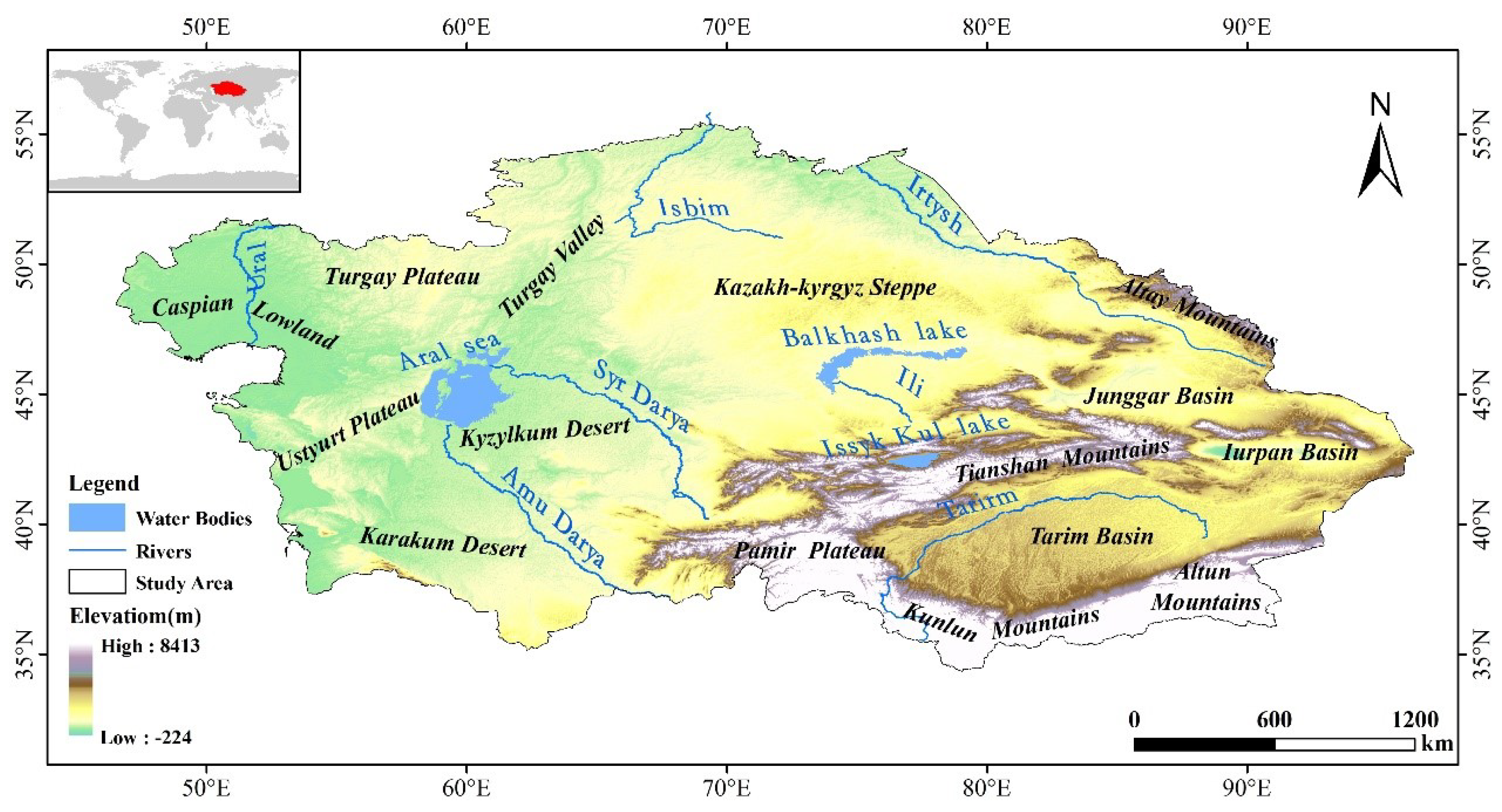
2.1. Study Area

Central Asia is located at the center of Asia and includes Kazakhstan, Kyrgyzstan, Tajikistan, Turkmenistan, Uzbekistan, and the Xinjiang region of China (Figure 1). It covers over 4 million square kilometers. Central Asia is geographically unique and features a diverse climate that ranges from extremely arid deserts to humid and mountainous regions. The dominant types of climate in the region are arid and semi-arid and render the distribution of vegetation and ecosystems in the area highly complex and diverse [21]. The vegetation cover mainly consists of grasslands, agricultural land, forests, and deserts, with grasslands and deserts being the most common. The grasslands are primarily located in central and northern Kazakhstan, the lowlands of Kyrgyzstan, and certain areas of Turkmenistan and Uzbekistan [22]. Forests are mainly concentrated in mountainous regions, such as the Tianshan Mountains, Altai Mountains, and Pamir Plateau, while vast desert areas are primarily located in the western parts of Turkmenistan and Uzbekistan, the southwestern part of Kazakhstan, and the Tarim and Junggar Basins in Xinjiang [23,24].

The climatic and topographical conditions have a significant impact on the distribution of local vegetation and changes in Central Asia [25]. Water resources in the region continue to deplete under the influence of global climate change. This, in conjunction with the degradation and desertification of land due to overgrazing, poses a serious threat to the vegetation cover [26]. Changes in the vegetation cover, particularly along the boundary between grasslands and deserts, are especially significant and jeopardize ecological security and sustainable development [27].

2.2. Datasets and Pre-Processing

We used datasets of the NDVI, EVI, NIRv, and kNDVI, along with gridded data on the regional temperature and precipitation.

The NDVI and EVI datasets were directly extracted from the MODIS MOD13Q1 product, released by NASA EOS Data Center (https://ladsweb.modaps.eosdis.nasa.gov, accessed on 30 January 2025). The MOD13Q1 product was generated every 16 days at a spatial resolution of 250 m. In addition to the NDVI and EVI layers, the MOD13Q1 product contains the MODIS reflectance band 2 (near-infrared), which is required to calculate the NIRv.

The NIRv was calculated as the product of the NDVI and NIR bands [14].

$$\mathrm{NIRv}=\mathrm{NIR}\times \mathrm{NDVI}$$

(1)

The kNDVI is a non-linear generalization of the NDVI.

$$\mathrm{kNDVI}=\tanh \left({\left({\displaystyle \frac{\mathrm{NIR}-\mathrm{Red}}{2\mathsf{\sigma }}}\right)}^2\right)$$

(2)

where $\sigma$ determines the distance between the NIR and red bands and is a tunable, length-scale parameter designed to capture the non-linear sensitivity of the NDVI to the density of vegetation. Following Camps-Valls et al. [15], its simplified formulation is = 0.5 (NIR + red). Then, Equation (2) can be simplified as follows:

$$\mathrm{kNDVI}=\tanh \left({\mathrm{NDVI}}^2\right)$$

(3)

To further reduce the impact of errors in the atmospheric data, the maximum value composite method [28] was applied to reproduce data on the NDVI, EVI, NIRv, and kNDVI at an annual scale. Pixels with values of the NDVI smaller than 0.1 were considered to represent unvegetated areas and were removed.

In addition to the above data, we used the entropy weighting method [29,30] to combine the four indices—NDVI, EVI, NIRv, and kNDVI—and construct a composite index, the CVI:

$${\mathrm{CVI}}_{\mathrm{t}}={\sum }_{\mathrm{i}=1}^{\mathrm{n}}\left({\mathrm{W}}_{\mathrm{i}}\times {\mathrm{VI}}_{\mathrm{it}}\right)$$

(4)

$${\mathrm{W}}_{\mathrm{i}}={\displaystyle \frac{1-{\mathrm{e}}_{\mathrm{i}}}{{\sum }_{\mathrm{i}=1}^{\mathrm{n}}\left(1-{\mathrm{e}}_{\mathrm{i}}\right)}}$$

(5)

where CVI_t is the CVI at time t, VI_it is the value of the i-th index at time t, W_i is the weight of the i-th index, e_i represents the informational entropy of the i-th index, and n is the total number of indices, four. The range of values of the CVI is [0, 1], with higher values indicating greater vegetation cover.

Gridded datasets of the annual total precipitation (PRE) and mean temperature (TMP) in the growing season (April–October) were obtained at a spatial resolution of 0.5° from the Climate Research Unit Version 4.03 (CRU TS4.03). They were used to test the correlation between the vegetation indices and hydrothermal factors. The spatial resolutions of the vegetation indices were resampled to 0.5° to match the CRU data.

2.3. Data Analysis

We systematically compared the four indices with the CVI in terms of their patterns of spatial distribution, trends of changes, spatiotemporal heterogeneity, and correlations with the temperature and precipitation. The spatial patterns of the vegetation were expressed by using the multi-year averages of the NDVI, EVI, NIRv, kNDVI, and CVI from 2000 to 2022. The trends of changes in the indices were checked by using the Mann–Kendall non-parametric test, while their spatiotemporal heterogeneity was quantified by using the coefficient of variation (CV). We employed a moving window with a size of 15 × 15 pixels (i.e., 225 pixels were included) to calculate the spatial CV (CVs) [29]. The moving window was separately applied to the annually averaged images of the indices. The temporal CV (CVt) over 2000–2022 was calculated at the pixel scale. The coefficient of partial correlation was used to measure the correlation between the indices and the precipitation and temperature.

3. Results

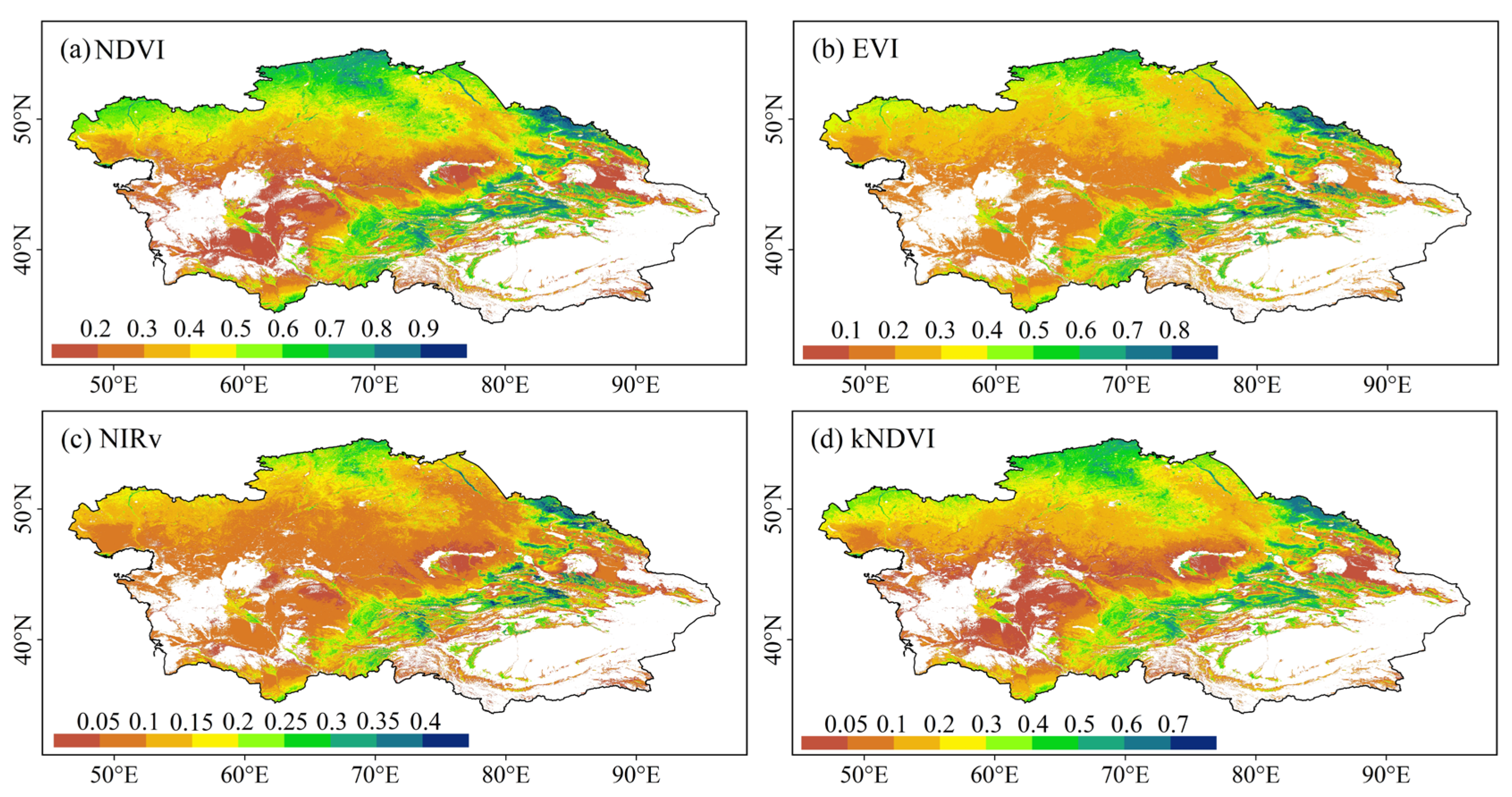
3.1. Spatiotemporal Variations in NDVI, EVI, NIRv, and kNDVI

Figure 2 shows that the spatial patterns of the NDVI, EVI, NIRv, and kNDVI in Central Asia were generally similar and exhibited distinct variations with the elevation. Overall, there was extensive vegetation coverage in humid mid-mountain areas, which received abundant precipitation and had a suitable temperature. The values of the NDVI, EVI, NIRv, and kNDVI in the Altai Mountains, Tianshan Mountains, Pamir Plateau, Kazakh–Kyrgyz Steppe, Turgay Plateau, and downstream areas of the Isbim River were >0.5, >0.3, >0.15, and >0.2, respectively. By contrast, vegetation growth was constrained by cold temperatures in mountainous areas above 3500 m, where winters are long and temperatures are low, and led to lower values of the NDVI, EVI, NIRv, and kNDVI of <0.4, <0.3, <0.15, and <0.2, respectively. Moreover, vegetation coverage was generally low in arid areas at a low elevation where precipitation was scarce, including the Tarim Basin, Junggar Basin, Karakum Desert, Caspian Lowland, and areas surrounding the Aral Sea.

The annual regional average values of the NDVI, EVI, NIRv, and kNDVI in 2000–2022 were calculated from the time series of image-related data to analyze the interannual variations in them. Figure 3 shows that all four indices exhibited consistent interannual fluctuations, with the minimum values recorded in 2008 and 2016, and the maximum values occurring in 2002 and 2007. However, an analysis of their trends suggested that the values of the NDVI and EVI had increased, with values of the Mann–Kendall statistic Zc of 0.37 and 0.58, respectively. Neither of these values reached significance, however (p > 0.05). By contrast, the NIRv and kNDVI both exhibited a trend of decrease, with values of Zc of −0.05 and −0.69, respectively. Neither was statistically significant (p > 0.05).

We applied Mann–Kendall tests to the time series of images at the pixel scale for spatial analysis. Figure 4 shows that the spatial distributions of the patterns of changes in the four indices were generally consistent, with regions exhibiting overlapping trends of increase or decrease. Areas in which their values increased were primarily concentrated in the central region with low vegetation coverage, such as areas around the Tarim Basin, while areas in which the values of the indices decreased were mainly distributed in regions with higher vegetation coverage. They included the western Tianshan Mountains, Turgay Plateau, Isbim River Basin, and downstream areas of Irtysh River.

However, there were differences in the sizes of areas in which the values of the indices exhibited different trends of change. The value of the NDVI increased over a much larger area than the other three indices, while that of the kNDVI significantly decreased over a much larger area. The ratios of areas that recorded significant changes (|Zc| > 1.96) in values of the NDVI and kNDVI were 18.28% and 17.30%, respectively. The NDVI significantly increased (Zc > 1.96) in 12.60% of the region and significantly decreased in 5.67%. The value of the kNDVI significantly increased (Zc > 1.96) over 8.28% of the area and significantly decreased (Zc < −1.96) in 9.01%. The ratios of areas that had undergone significant changes (|Zc| > 1.96) in values of the EVI and NIRv were 15.06% and 13.58%, respectively. Among them, the EVI significantly increased (Zc > 1.96) in 10.57% of the region and significantly decreased (Zc < −1.96) in only 4.49%. The value of the NIRv significantly increased (Zc > 1.96) in 8.05% of the region and significantly decreased in 5.54%.

When we overlaid the types of changes in the trends of the indices in a pairwise manner, we found that the difference between the NDVI and NIRv was the largest, with their area ratios exhibiting different but significant trends of change (p < 0.05) that reached 13.57%. Among them, the area in which the NDVI significantly increased while the NIRv showed no significant change accounted for 6.41% of the total (Figure 5 and Figure 6b). The ratio of areas in which the EVI and kNDVI and the NIRv and kNDVI exhibited different trends reached 12.87% and 12.16%, respectively. The difference between the EVI and NIRv was the smallest (i.e., they were the most similar), with the ratio of area in which they exhibited different trends of changes at 8.63%. The ratio of the area in which the NDVI and kNDVI had different trends of changes was 9.93%.

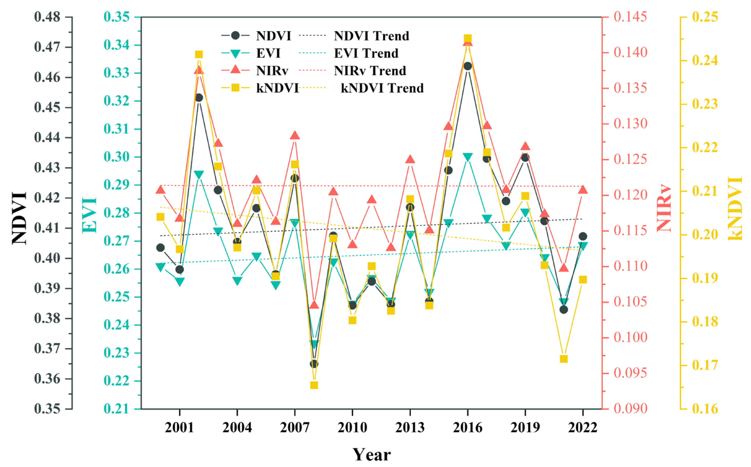
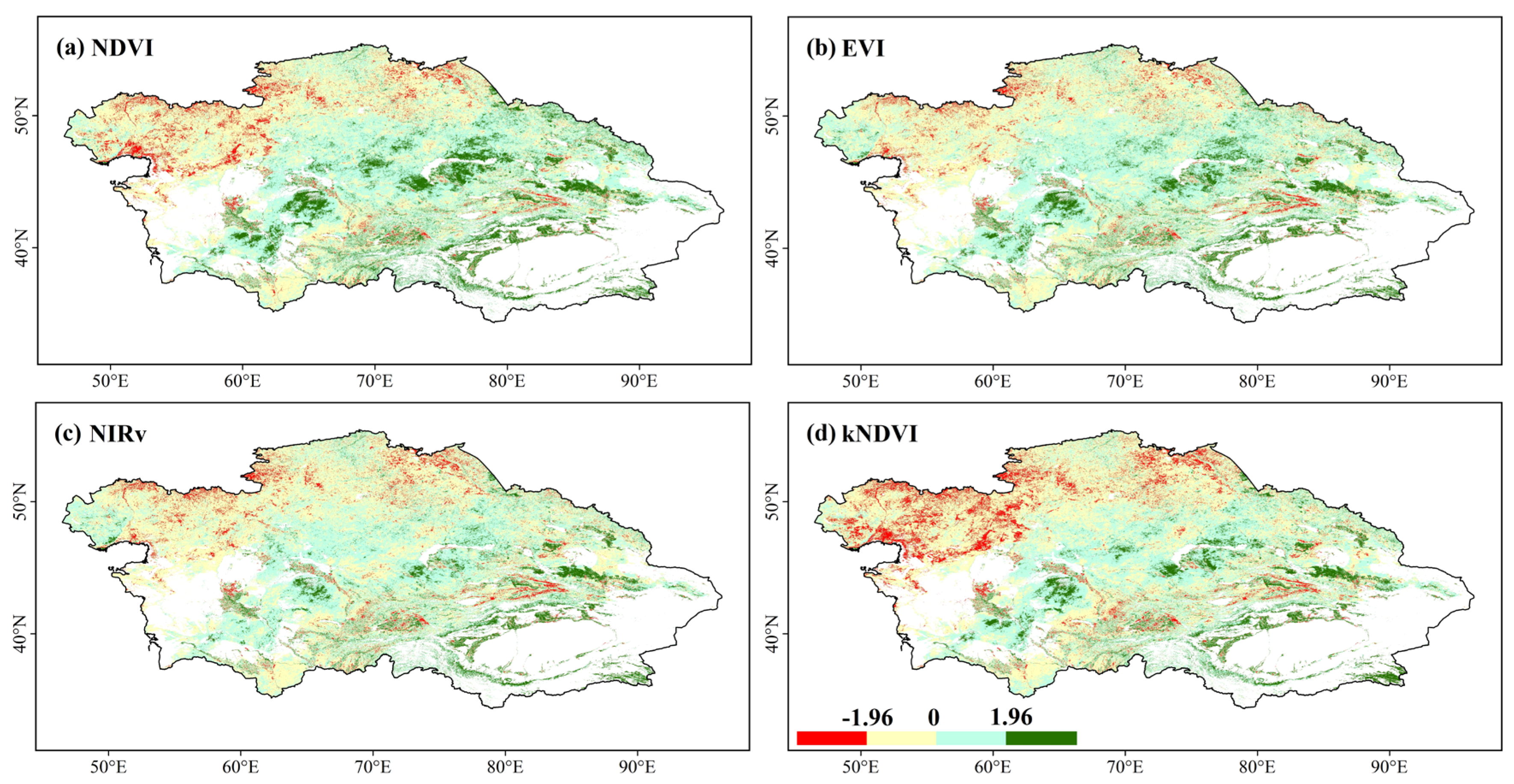
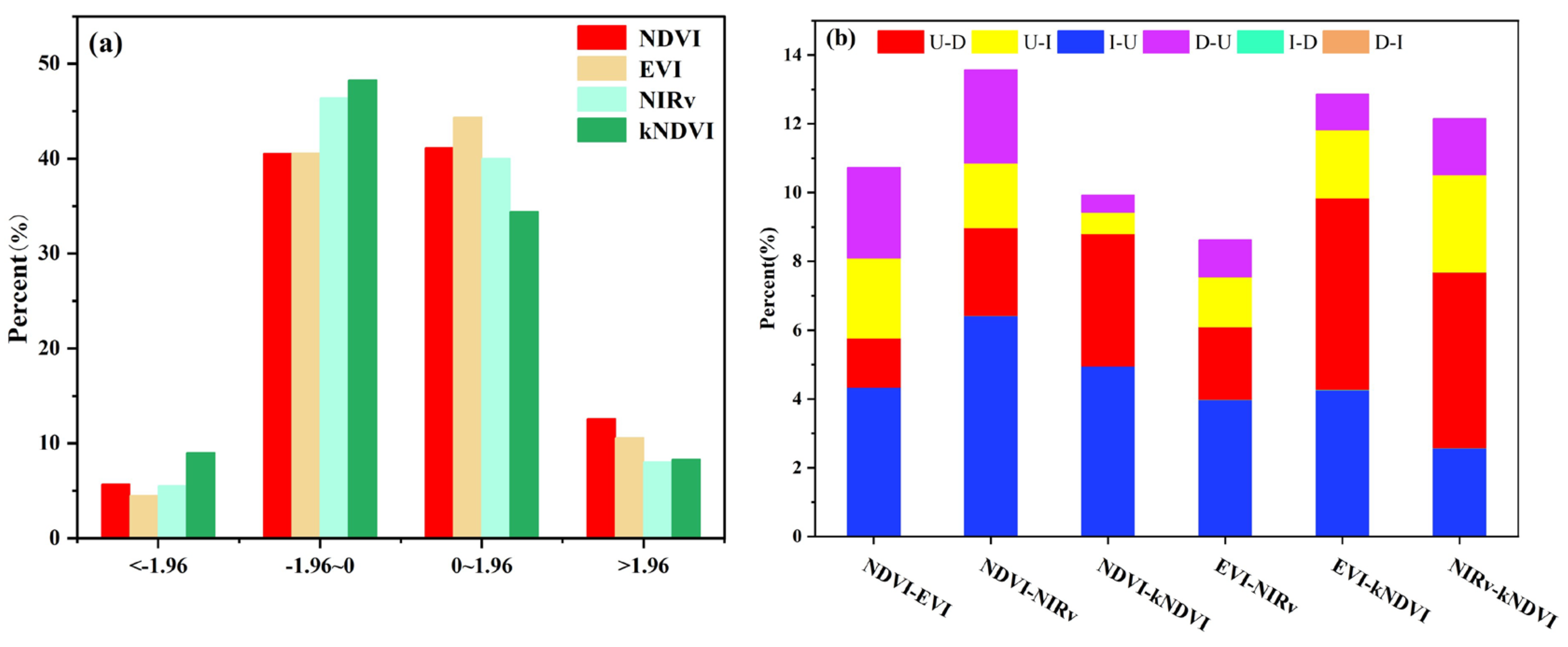
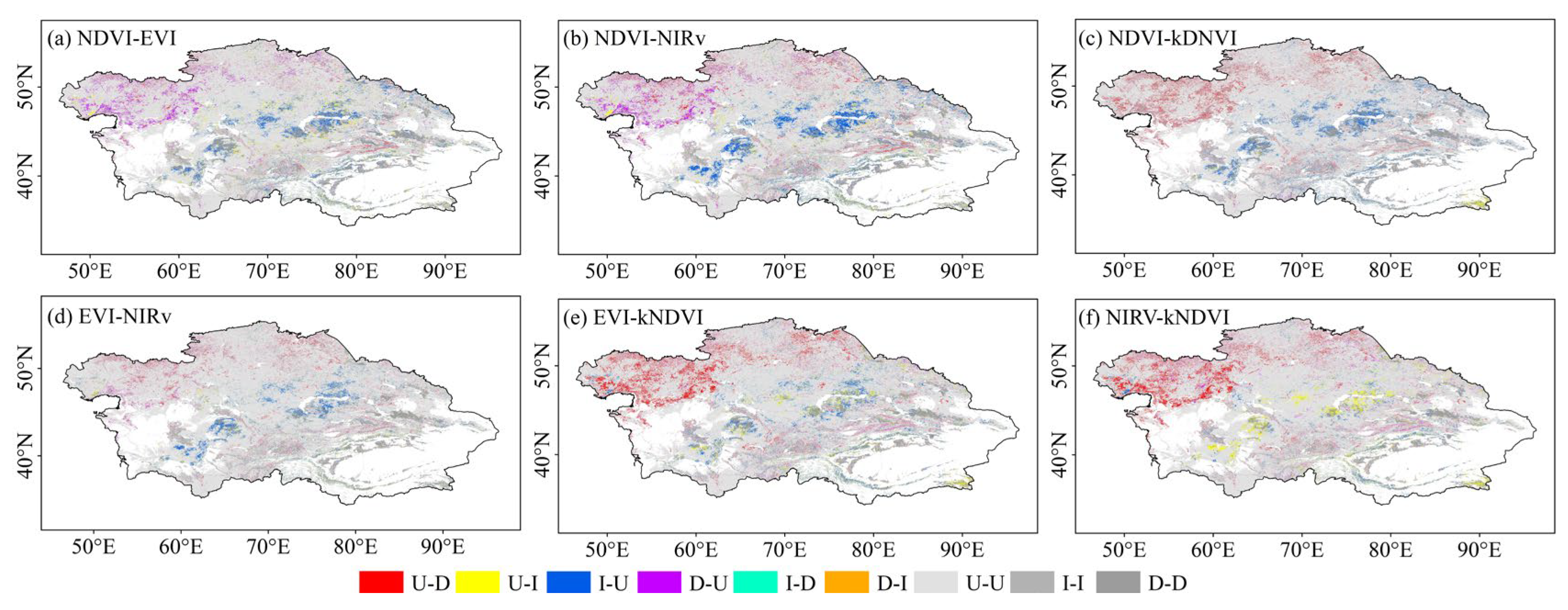
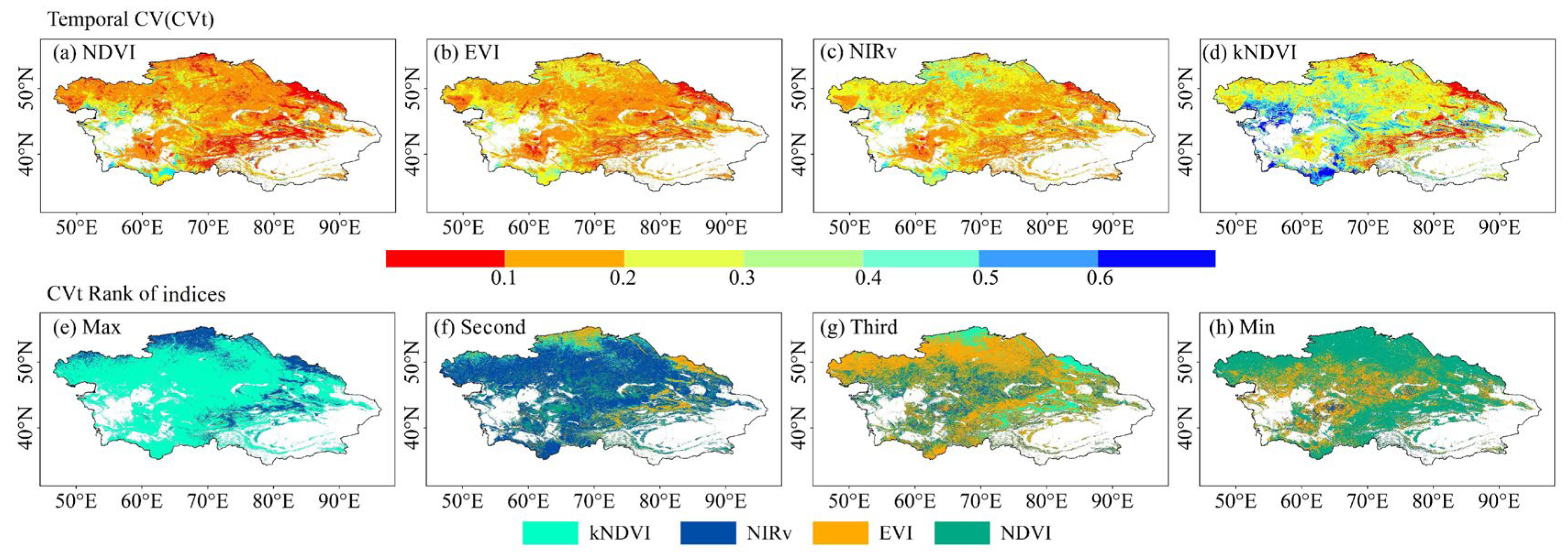
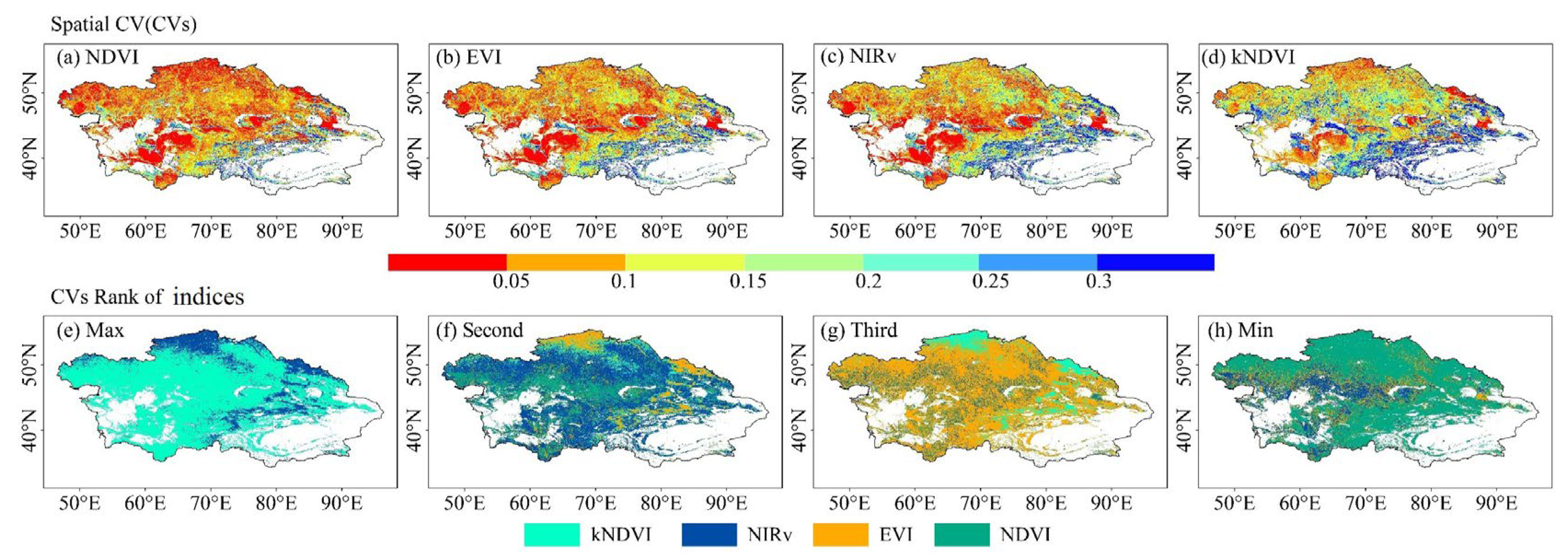
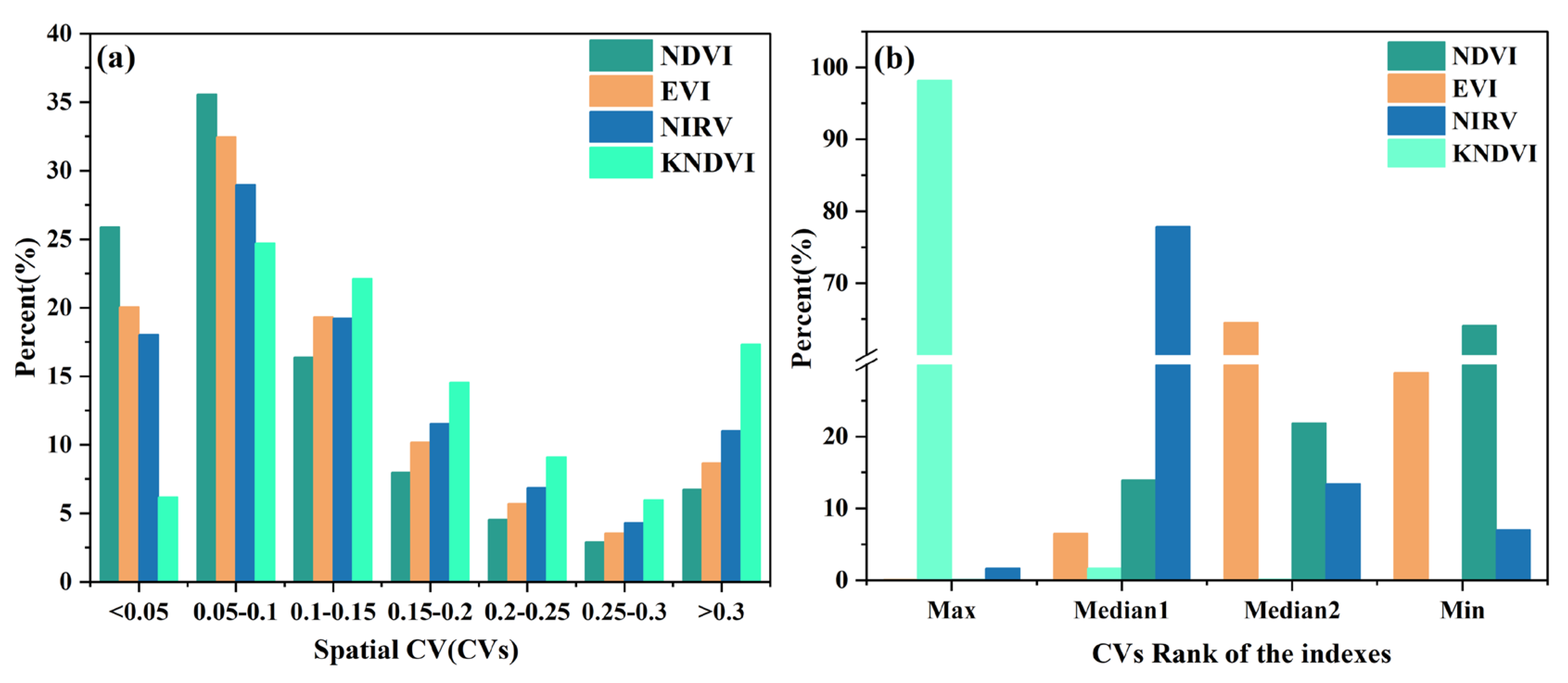
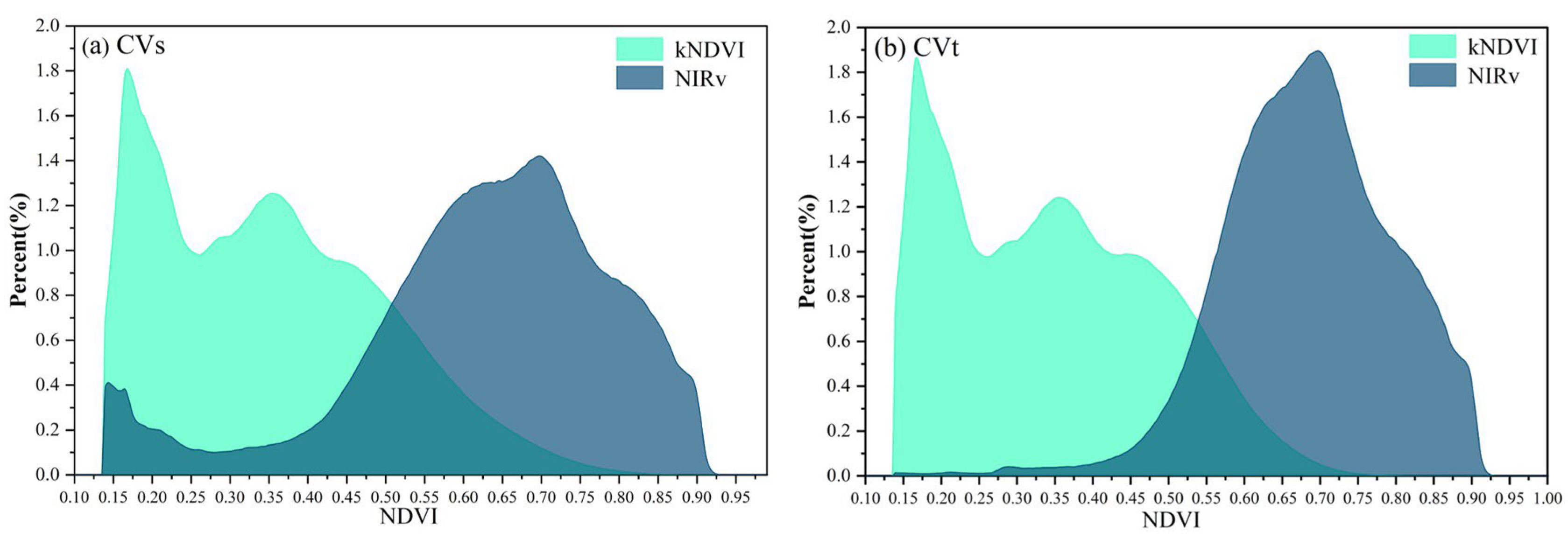
3.2. Comparison Between the Spatial and Temporal Heterogeneity of NDVI, EVI, NIRv, and kNDVI

The CVt rankings in Figure 7 show that the kNDVI had the highest ratio of areas with the maximum CVt among the four indices (Figure 7e), and its CVt was greater than those of the other three indices in 81.65% of the study area. The NIRv accounted for 17.20% (Figure 7b). The NDVI had the smallest CVt (Figure 7h), with a ratio of 63.99%, while EVI accounted for 28.86% (Figure 8b). The NIRv had the second-largest CVt (Figure 7f), with a proportion of 62.95%, while the NDVI, EVI, and kNDVI accounted for 13.89%, 13.91%, and 9.25%, respectively. The EVI had the third-largest CVt (Figure 7g), with a ratio of 56.21%, while the NDVI accounted for 21.99% (Figure 8b). Thus, the four indices were ranked as kNDVI > NIRv > EVI > NDVI in terms of their ability to express the temporal CV of vegetation coverage.

The map of CVt in Figure 7 shows that the values of the NDVI, EVI, NIRv, and kNDVI decreased sequentially in areas with CVt < 0.2 and increased sequentially in areas with CVt > 0.2. The values of the kNDVI were notably larger than those of the other three indices in areas with CVt > 0.5. The area ratios in maps of the spatial distributions of the NDVI, EVI, NIRv, and kNDVI were 14.69%, 8.26%, 3.69%, and 5.23%, respectively, for CVt < 0.1. Their area ratios for 0.1 < CVt < 0.2 were 59.83%, 59.06%, 47.20%, and 13.49%, respectively, while those for 0.2 < CVt < 0.3 were 19.71%, 24.39%, 33.25%, and 34.47%, respectively. The area ratios of the NDVI, EVI, NIRv, and kNDVI for 0.3 < CVt < 0.4 were 4.31%, 6.37%, 11.20%, and 24.48%, while those for 0.4 < CVt were 1.45%, 1.92%, 4.65%, and 22.32%, respectively.

It is evident from the CVs map in Figure 9 that the NDVI, EVI, NIRv, and kNDVI decreased sequentially in areas with CVs < 0.1 and increased sequentially in areas with CVs > 0.20. The area ratios of NDVI, EVI, NIRv, and kNDVI for CVs < 0.05 were 25.91%, 20.06%, 18.05%, and 6.20%, respectively; were 35.56%, 32.47%, 28.98%, and 24.70% for 0.05 < CVs < 0.10; had values of 6.75%, 8.69%, 11.01%, and 17.32%, respectively, for CVs > 0.35; and were 2.90%, 3.54%, 4.31%, and 5.96%, respectively, for 0.30 < CVs < 0.35.

Figure 9e shows that the kNDVI had the highest ratio of areas with the maximum CVs, 79.47%, while the NIRv accounted for 20.22% (Figure 10b). The NDVI had the smallest CVs (Figure 9h), with a ratio of 67.98%. The NIRv had the second-largest CVs (Figure 9f), with a ratio of 52.77%, while the NDVI, EVI, and kNDVI accounted for 22.44%, 14.05%, and 10.74%, respectively. The EVI had the third-largest CVs (Figure 9g), with a ratio of 71.70%, while each of the other three indices accounted for around 9.50%.

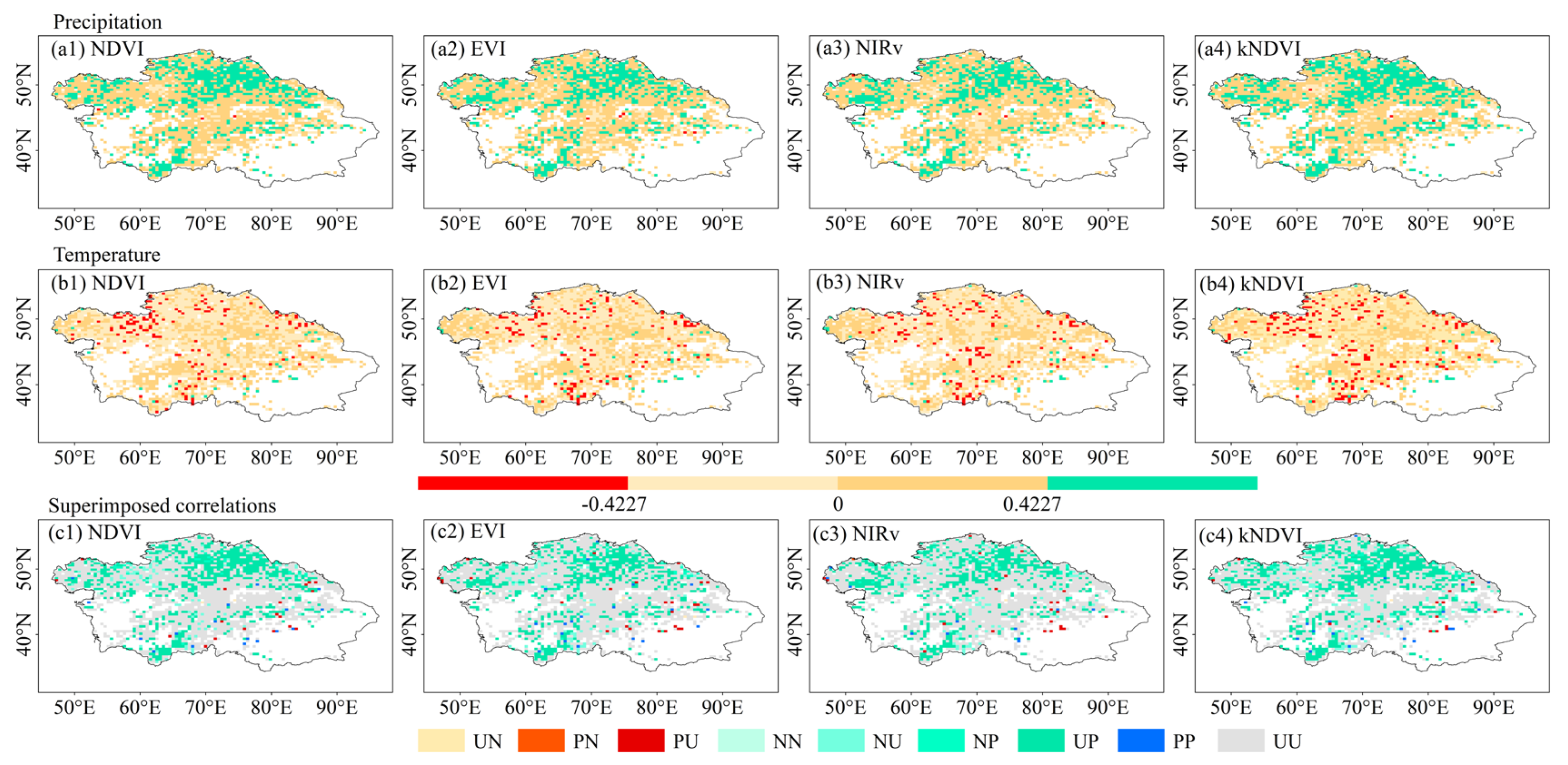
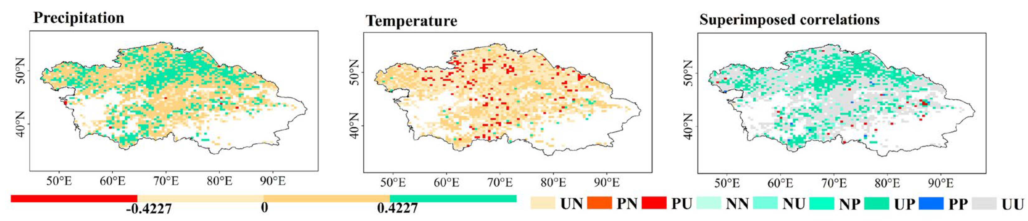
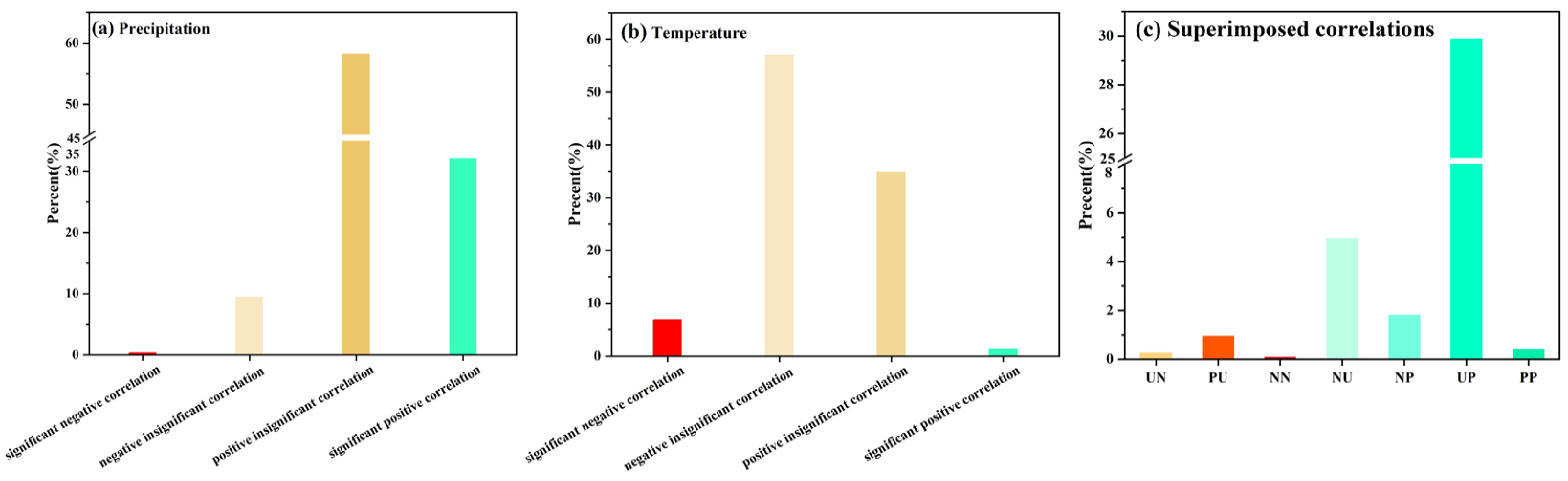
3.3. Correlation Between the Indices, and Temperature and Precipitation

As shown in Figure 11 and Figure 12, the interannual variations in vegetation cover in Central Asia exhibited a prominently higher correlation with the precipitation than with the temperature, with a predominantly positive correlation with the former and a negative correlation with the latter. The ratios of areas for the four indices that were positively correlated with the precipitation ranged from 87.69% to 91.04% (Figure 12a), while the ratios that were negatively correlated with the temperature ranged from 59.71% to 65.11% (Figure 12b). The ratios of a significantly positive correlation (p < 0.05) between the NDVI, EVI, NIRv, and kNDVI, and the precipitation were 30.96%, 28.10%, 26.67%, and 34.31%, respectively, with the kNDVI exhibiting the highest value. The ratios of the four indices exhibiting a significantly negative correlation (p < 0.05) with the precipitation were minor and ranged from 0.12% to 0.25% (Figure 12a). The ratios of significantly positive correlations (p < 0.05) with the temperature were also minor, ranging from 1.39% to 1.80%, while those of a significantly negative correlation with the temperature were higher, ranging from 5.93% to 8.14%. The kNDVI had a notably higher ratio than the other three indices (Figure 12b). When overlaying the correlations between the four indices and the temperature and precipitation, we observed that the UP category had the highest ratios of significant correlations with either the temperature or precipitation (Figure 12c), with values of 28.71%, 25.77%, 24.74%, and 31.53%, respectively. The ratios of their significant negative correlations with the temperature and non-significant positive correlations with the precipitation (NU category) were 4.34%, 4.25%, 4.29%, and 6.18%, respectively. Among them, the kNDVI had a higher ratio than the other three indices. It is evident that the kNDVI could better represent the correlations between the vegetation cover and the precipitation and temperature than the other three indices.

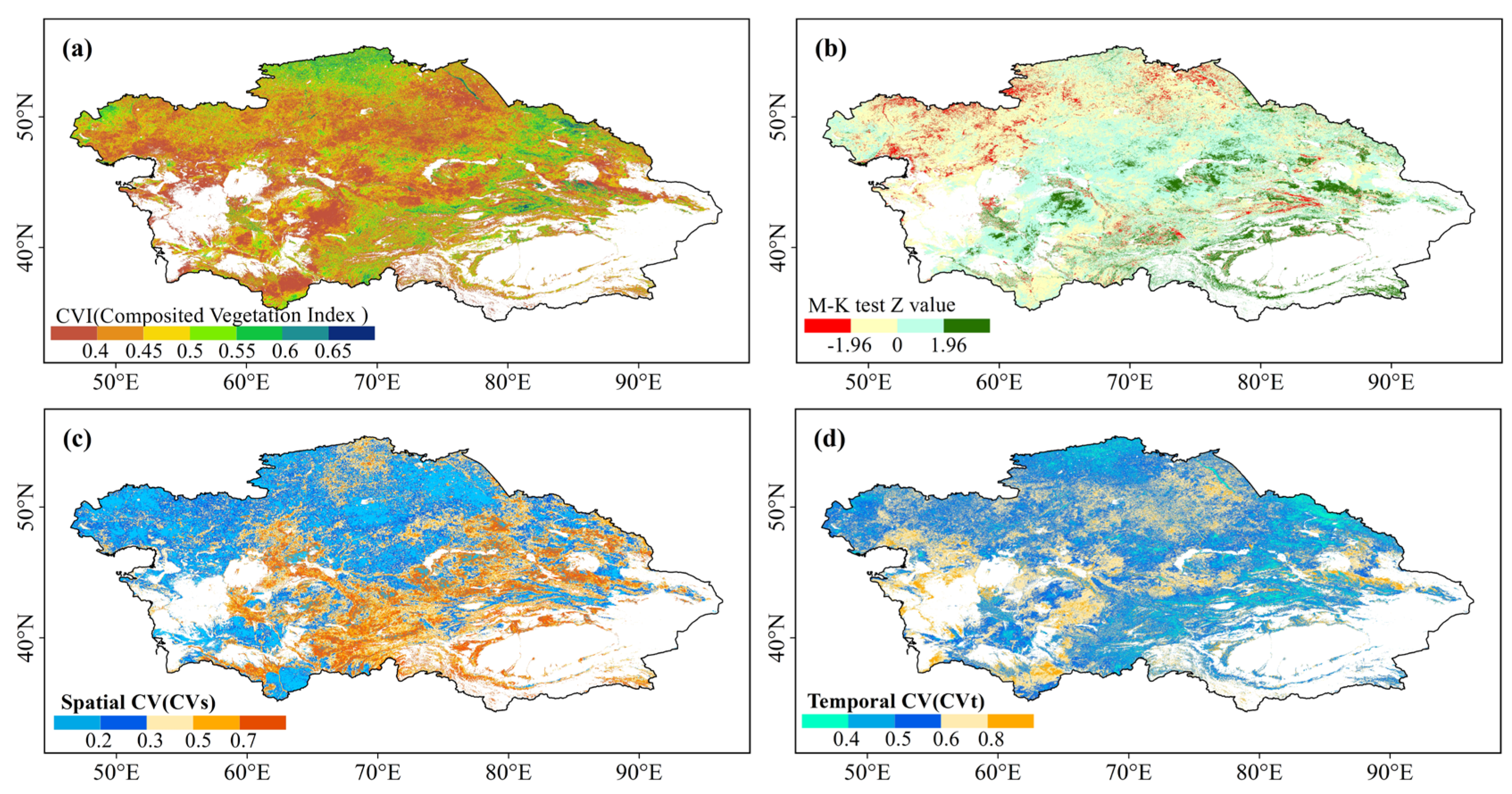
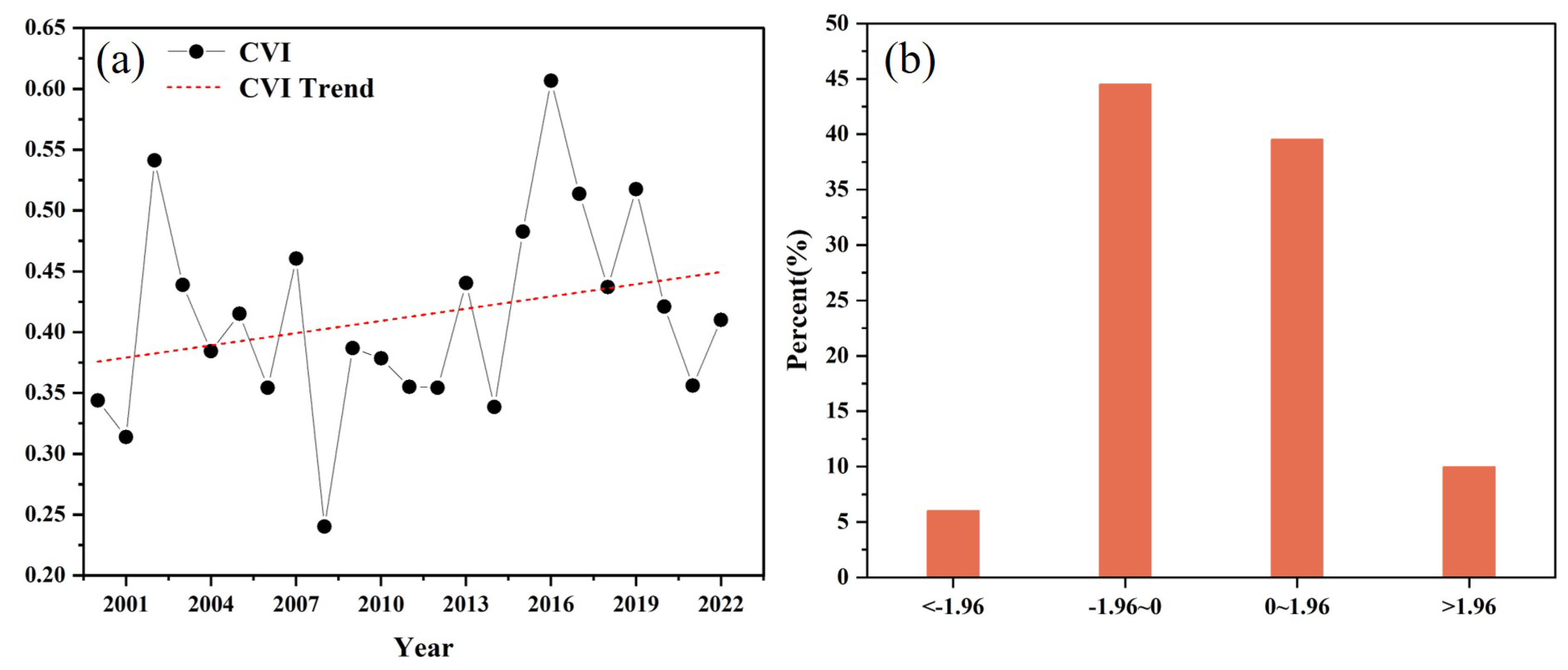
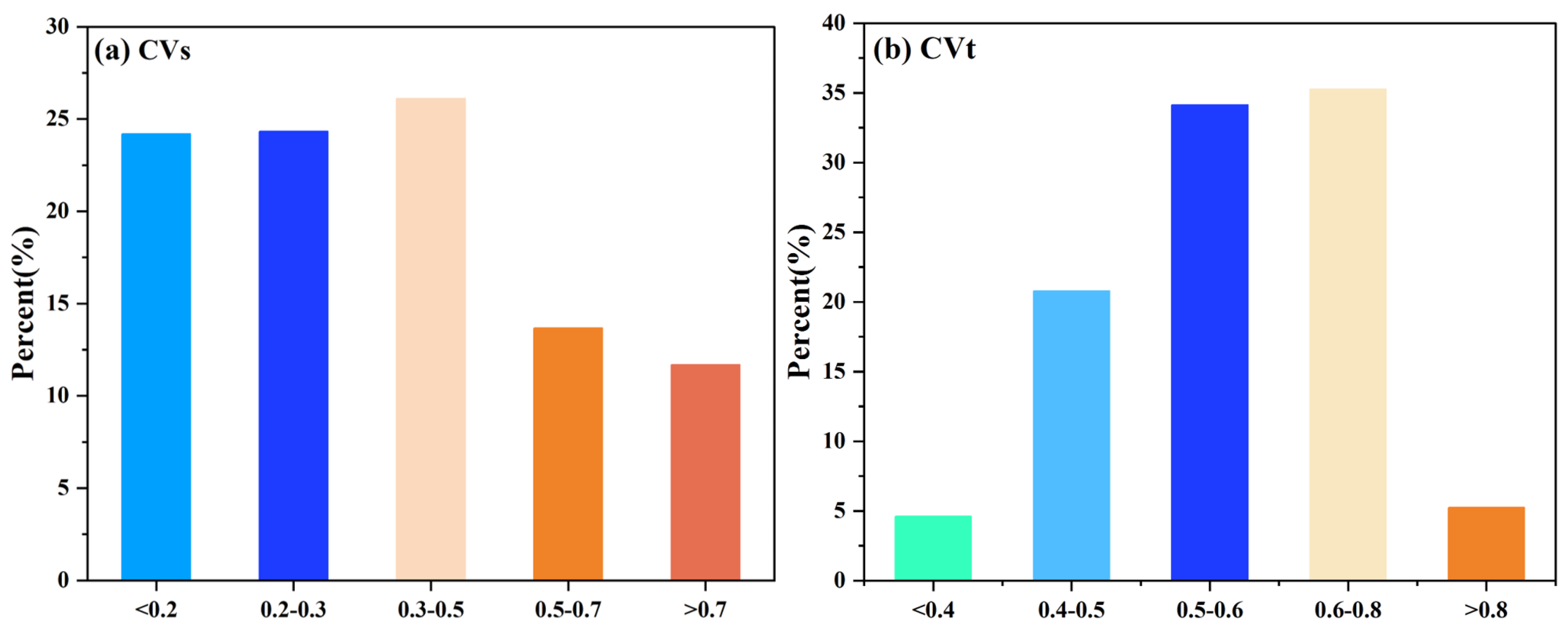
3.4. Comparison of CVI of NDVI, EVI, NIRv, and kNDVI

Figure 13 shows that the CVI was similar to the other four indices in terms of the spatial pattern of vegetation cover in the study area. The high-value areas for all four indices corresponded to those for the CVI. The overall trend in values of the CVI in the entire study area was one of a non-significant increase (Zc = 1.16 < 1.96) (Figure 14a). The ratio of area in which it underwent significant changes (|Z| > 1.96) was 15.99%, with 9.96% of this exhibiting a significant increase (Zc > 1.96) and 6.03% showing a significant decrease (Zc < −1.96) (Figure 14b). It thus did not boast a clear comparative advantage over the other indices.

The ratio of CVI with CVs > 0.3 was 51.47% (Figure 15a), while the corresponding proportions in the NDVI, EVI, NIRv, and kNDVI were only between 6.75% and 17.32% (Figure 10a). A total of 77.67% to 98.55% of the area for the four indices had values of CVt < 0.4 (Figure 8a), while only 4.60% had values of CVt < 0.4. Overall, the CVI was clearly superior to the other four indices in expressing spatiotemporal heterogeneity.

Figure 16 and Figure 17 show that the CVI had a higher correlation with the precipitation than with the temperature. Further analysis revealed that the total area over which the CVI had a significant correlation with either the temperature or the precipitation was 38.30%, while the corresponding values for the NDVI, EVI, NIRv, and kNDVI were 36.16%, 33.62%, 32.07%, and 41.19%, respectively. The ratio of the kNDVI was the highest, but the CVI surpassed the other three indices.

Specifically, 6.83% of the values of the CVI exhibited a significant negative correlation with the temperature, while 32.08% of it yielded a significant positive correlation with the precipitation. These values were lower than those for the kNDVI but higher than those for the other three indices. This shows that the CVI integrates the four indices, which means that it can be used as a composite index to analyze the relationship between changes in the vegetation cover and the temperature or precipitation.

4. Discussion

Central Asia is located in the heart of the Eurasian continent, has a dry and hot climate, and receives little rainfall. Its topography and latitude play a significant role in regulating its precipitation and temperature. The distribution of vegetation in the region exhibits a distinct altitudinal and latitudinal zonality. Restricted by a high temperature and scarce rainfall, desert vegetation prevails in its plains, with low vegetation coverage in areas around the Aral Sea, Tarim Basin, and Junggar Basin. By contrast, its mountainous areas and high-latitude regions in the north receive abundant precipitation and have a lower temperature. The water resources and temperature are thus suitable for the growth of vegetation, which mainly comprises meadows, coniferous forests, and broad-leaf forests [31]. Moreover, the regulation of precipitation and temperature by the topography and latitude of Central Asia also determines the correlation between them and the vegetation cover [32]. Except for some high mountainous regions, vegetation growth is limited by an insufficient water supply [33]. Vegetation growth is sensitive to changes in the precipitation and is positively correlated with it [34]. An increase in the temperature during the growing season limits plant growth, whereas a rise in the temperature accelerates evapotranspiration to accelerate water loss, especially in plains dominated by desert plants.

More than 100 vegetation indices have been developed in research thus far [35,36]. Most studies tend to use a single index when quantifying vegetation dynamics, but different indices have their own advantages and disadvantages in terms of representing the status of its growth [37,38]. The use of a single index may lead to misjudgment. For instance, Yan et al. [30] found that 28.69% of the grassland in the Ili Valley exhibited varying trends of changes over 2000–2019, as indicated by the TI-NDVI and NDVImax. Our analysis also revealed that although the NDVI, EVI, NIRv, and kNDVI were relatively consistent in expressing the spatial differences in vegetation coverage, they yielded significant differences in expressing the trends of changes in the vegetation and its spatiotemporal heterogeneity, as well as their correlations with the temperature and precipitation. Therefore, a method that combines multiple indices is recommended for more accurately representing the dynamic status of vegetation.

Furthermore, an analysis of Figure 7e and Figure 9e reveals that although the values of CVs and CVt of the kNDVI and NIRv were the largest in most parts of the vegetated region of Central Asia, there were significant differences between them. When NDVI > 0.50, the values of CVs of the NIRv were the largest in most areas (Figure 18a), while when NDVI > 0.54, the values of CVt of the NIRv were the largest in most areas (Figure 18b). It is evident that the NIRv had the largest values of CVs and CVt in areas with a high vegetation coverage, while the kNDVI had the largest CVs and CVt in areas with low vegetation coverage.

To balance the advantages and disadvantages of multiple indices, it is good practice to combine them into a comprehensive index by using objective methods of weighting them. The Remote Sensing Ecological Index (RSEI), which is widely used to quantify the overall ecological environment, is representative of this [39,40]. We used the entropy weighting method in this study to integrate the NDVI, EVI, NIRv, and kNDVI to construct the CVI. It significantly outperformed each of the four indices in terms of expressing the spatiotemporal heterogeneity of vegetation cover. Moreover, the values of the kNDVI and NDVI reflected significant changes and correlations with the temperature and precipitation over a larger proportional area compared with the EVI and NIRv. Although the ratios of significant changes and correlations represented by the CVI were lower than those of the kNDVI and NDVI, they were still higher than those of the EVI and NIRv. The CVI thus delivers superior results to those of the four individual indices.

Although vegetation indices such as time series NDVI of MODIS, Global Inventory Modeling and Mapping Studies (GIMMS), and The Global Land Surface Satellite (GLASS) have been widely recognized and applied in lots of studies, the limitations of those indices should not be overlooked [41,42]. This study revealed that 13.57% of the study area exhibited divergent changing trends between NDVI and NIRv, while the proportion also reached 12.87% when comparing EVI and kNDVI. In the absence of comprehensive ground-truth information, the definitive conclusions remain elusive [43,44]. This shows an under-explored aspect in the widespread applications of different vegetation indices, which requires further investigation [45]. Furthermore, these findings highlight that the selection of vegetation indices exerts substantial impacts on the research results of the dynamics of vegetation growth, indicating that comprehensive consideration is absolutely necessary when selecting indices.

5. Conclusions

In this study, Central Asia was selected as the research area to systematically compare four satellite-derived vegetation indices: the NDVI, EVI, NIRv, and kNDVI. We also combined them based on the entropy weighting method to construct the CVI and used it to determine the spatial distribution of changes in vegetation coverage, its spatiotemporal heterogeneity, and its correlations with the temperature and precipitation. We found that the NDVI, EVI, NIRv, and kNDVI as well as the CVI for Central Asia revealed similar spatial patterns of changes in vegetation cover in general. The kNDVI and NIRv generally reflected a non-significant decreasing trend of interannual changes in vegetation (p > 0.05), while the NDVI, EVI, and CVI generally showed a non-significant increasing trend of changes (p > 0.05). The spatial ratios of significant changes (negative or positive) according to the NDVI and kNDVI were 18.28% and 17.30%, respectively, while those of the EVI and NIRv were 15.06% and 13.58%, respectively. The kNDVI recorded results that were different from those of the EVI and NIRv but similar to those of the NDVI. The NIRv yielded different results from those of the NDVI and kNDVI but similar to those of the EVI. The values of the kNDVI of 81.65% and 79.47% for the vegetated region of Central Asia yielded the largest values of CVt and CVs among the four indices, followed by the NIRv. The NIRv and kNDVI were best able to represent areas with high and low vegetation coverage, respectively. The critical value of the NDVI for distinguishing between the temporal heterogeneity (CVt) of high and low vegetation cover was 0.54, while that for spatial heterogeneity (CVs) was 0.50. The kNDVI had a much better ability than the other three indices to express the correlation between the vegetation cover and the temperature and precipitation. The values of the kNDVI of 41.19% for the vegetated region of Central Asia exhibited a significant correlation (negative or positive) with either the temperature or precipitation, compared with 36.16%, 33.62%, and 32.07% for the NDVI, EVI, and NIRv, respectively. Around 15.99% of the values of the CVI reflected significant changes (negative or positive), while 38.30% of its values were significantly correlated (negatively or positively) with the temperature or precipitation. This means that the CVI exhibited no prominent comparative advantage over the other indices in terms of representing changes in vegetation cover or correlations with the temperature or precipitation. The ratios of values of CVs > 0.3 or CVt > 0.4 of the CVI were 51.47% and 95.40%, respectively. This shows that the CVI was clearly superior to the other four indices in terms of expressing the spatiotemporal heterogeneity of vegetation cover in Central Asia.

References

1. Huang, J.P.; Yu, H.P.; Guan, X.D.; Wang, G.Y.; Guo, R.X. Accelerated dryland expansion under climate change. Nat. Clim. Change 2016, 6, 166–171. [Google Scholar] [CrossRef]
2. Lewin, A.; Murali, G.; Rachmilevitch, S.; Roll, U. Global evaluation of current and future threats to drylands and their vertebrate biodiversity. Nat. Ecol. Evol. 2024, 8, 1448–1458. [Google Scholar] [CrossRef] [PubMed]
3. de Oliveira, M.L.; dos Santos, C.A.C.; de Oliveira, G.; Perez-Marin, A.M.; Santos, C.A.G. Effects of human-induced land degradation on water and carbon fluxes in two different Brazilian dryland soil covers. Sci. Total Environ. 2021, 792, 148458. [Google Scholar] [CrossRef] [PubMed]
4. Yin, P.; Li, C.H.; Wei, Y.F.; Zhang, L.; Liu, C.; Chen, J.H.; Liu, Y.F.; Xiong, X.T. Impact of relative temperature changes on vegetation growth in China from 2001 to 2017. J. Clean. Prod. 2024, 451, 142062. [Google Scholar] [CrossRef]
5. Chen, Z.; Liu, J.Y.; Hou, X.T.; Fan, P.Y.; Qian, Z.H.; Li, L.; Zhang, Z.S.; Feng, G.L.; Li, B.L.; Sun, G.Q. Detection and Attribution of Greening and Land Degradation of Dryland Areas in China and America. Remote Sens. 2023, 15, 2688. [Google Scholar] [CrossRef]
6. Hou, L.; Xi, W.M.; Zhang, S.X. Effect of Understory on a Natural Secondary Forest Ecosystem Carbon Budget. Russ. J. Ecol. 2015, 46, 51–58. [Google Scholar] [CrossRef]
7. Cong, W.W.; Li, X.Y.; Pan, X.B.; Liu, X.P.; Lu, Q.; Wang, F. A new scientific framework of dryland ecological quality assessment based on 1OAO principle. Ecol. Indic. 2022, 136, 108595. [Google Scholar] [CrossRef]
8. Dacal, M.; García-Palacios, P.; Asensio, S.; Cano-Díaz, C.; Gozalo, B.; Ochoa, V.; Maestre, F.T. Contrasting mechanisms underlie short- and longer-term soil respiration responses to experimental warming in a dryland ecosystem. Glob. Change Biol. 2020, 26, 5254–5266. [Google Scholar] [CrossRef]
9. Lu, G.; Chen, X.; Wang, J.; Wu, C. Research Progresses on the Effects of Global Change on the Microbes of Plant-site Interface in Alpine Grassland Ecosystem. Acta Agrestia Sin. 2014, 22, 234–242. [Google Scholar]
10. Gorji, T.; Sertel, E.; Tanik, A. Monitoring soil salinity via remote sensing technology under data scarce conditions: A case study from Turkey. Ecol. Indic. 2017, 74, 384–391. [Google Scholar] [CrossRef]
11. Zhiqiang, W.; Baoyuan, L.I.U.; Chunxing, H.A.I. Effects of Soil Depth on Vegetation Cover and Above Ground Biomass in East Part of Inner Mongolia. J. Soil Water Conserv. 2007, 21, 164–167. [Google Scholar]
12. Linderholm, H.W. Growing season changes in the last century. Agric. For. Meteorol. 2006, 137, 1–14. [Google Scholar] [CrossRef]
13. Huete, A.; Didan, K.; Miura, T.; Rodriguez, E.P.; Gao, X.; Ferreira, L.G. Overview of the radiometric and biophysical performance of the MODIS vegetation indices. Remote Sens. Environ. 2002, 83, 195–213. [Google Scholar] [CrossRef]
14. Badgley, G.; Field, C.B.; Berry, J.A. Canopy near-infrared reflectance and terrestrial photosynthesis. Sci. Adv. 2017, 3, e1602244. [Google Scholar] [CrossRef] [PubMed]
15. Camps-Valls, G.; Campos-Taberner, M.; Moreno-Martínez, A.; Walther, S.; Duveiller, G.; Cescatti, A.; Mahecha, M.D.; Muñoz-Marí, J.; García-Haro, F.J.; Guanter, L.; et al. A unified vegetation index for quantifying the terrestrial biosphere. Sci. Adv. 2021, 7, eabc7447. [Google Scholar] [CrossRef]
16. Gogoi, J.; Newlands, N.K.; Mehrabi, Z.; Coops, N.C.; Ramankutty, N. Assessing the Performance of Satellite-Based Models for Crop Yield Estimation in the Canadian Prairies. Can. J. Remote Sens. 2023, 49, 2252926. [Google Scholar] [CrossRef]
17. Rasul, A.; Balzter, H.; Smith, C. Diurnal and Seasonal Variation of Surface Urban Cool and Heat Islands in the Semi-Arid City of Erbil, Iraq. Climate 2016, 4, 42. [Google Scholar] [CrossRef]
18. Brenes, C.L.M.; Jones, K.W.; Schlesinger, P.; Robalino, J.; Vierling, L. The impact of protected area governance and management capacity on ecosystem function in Central America. PLoS ONE 2018, 13, e0205964. [Google Scholar] [CrossRef]
19. Zhao, R.F.; Wang, J.F.; Li, L.H.; Zhang, L.H.; Lu, H.T.; Jiang, X.Y.; Chen, X.D.; Han, Z.Y.; Cairang, D.Z.; Wang, H.; et al. Evaluation of alpine wetland ecological degradation based on alpine wetland degradation index: A case study in the first meander of the Yellow River. Ecol. Indic. 2024, 158, 111414. [Google Scholar] [CrossRef]
20. Wang, Y.; Zhang, K.; Li, F. Monitoring of fractional vegetation cover change in Xilingol League based on MODIS data over 10 years. J. Arid Land Resour. Environ. 2012, 26, 165–169. [Google Scholar]
21. Gao, C.; Ren, X.L.; Fan, L.L.; He, H.L.; Zhang, L.; Zhang, X.Y.; Li, Y.; Zeng, N.; Chen, X.Z. Assessing the Vegetation Dynamics and Its Influencing Factors in Central Asia from 2001 to 2020. Remote Sens. 2023, 15, 4670. [Google Scholar] [CrossRef]
22. Zhou, Y.; Zhang, L.; Xiao, J.F.; Williams, C.A.; Vitkovskaya, I.; Bao, A.M. Spatiotemporal transition of institutional and socioeconomic impacts on vegetation productivity in Central Asia over last three decades. Sci. Total Environ. 2019, 658, 922–935. [Google Scholar] [CrossRef] [PubMed]
23. Li, M.Y.; Yao, J.Q.; Zheng, J.H. Spatio-Temporal Change and Drivers of the Vegetation Trends in Central Asia. Forests 2024, 15, 1416. [Google Scholar] [CrossRef]
24. Lin, M.L.; Chen, C.W.; Wang, Q.B.; Cao, Y.; Shih, J.Y.; Lee, Y.T.; Chen, C.Y.; Wang, S. Fuzzy model-based assessment and monitoring of desertification using MODIS satellite imagery. Eng. Comput. 2009, 26, 745–760. [Google Scholar] [CrossRef]
25. Du, H.R.; Tan, M.L.; Zhang, F.; Chun, K.P.; Li, L.H.; Kabir, M.H. Evaluating the effectiveness of CHIRPS data for hydroclimatic studies. Theor. Appl. Climatol. 2024, 155, 1519–1539. [Google Scholar] [CrossRef]
26. Chen, T.; Bao, A.M.; Jiapaer, G.; Guo, H.; Zheng, G.X.; Jiang, L.L.; Chang, C.; Tuerhanjiang, L. Disentangling the relative impacts of climate change and human activities on arid and semiarid grasslands in Central Asia during 1982–2015. Sci. Total Environ. 2019, 653, 1311–1325. [Google Scholar] [CrossRef]
27. Sun, Y.L.; Shan, M.; Pei, X.R.; Zhang, X.K.; Yang, Y.L. Assessment of the impacts of climate change and human activities on vegetation cover change in the Haihe River basin, China. Phys. Chem. Earth 2020, 115, 102834. [Google Scholar] [CrossRef]
28. Holben, B.N. Characteristics of maximum-value composite images from temporal AVHRR data. Int. J. Remote Sens. 1986, 7, 1417–1434. [Google Scholar] [CrossRef]
29. Li, H.; Li, B.; Ge, L.; Han, C.; Yang, Q.; Zhang, Y. Temporal and Spatial Characteristics of Vegetation Evolution and Topographic Effects in Fenhe River Basin from 2000 to 2021. Ecol. Environ. Sci. 2023, 32, 439–449. [Google Scholar]
30. Yan, J.J.; Zhang, G.P.; Ling, H.B.; Han, F.F. Comparison of time-integrated NDVI and annual maximum NDVI for assessing grassland dynamics. Ecol. Indic. 2022, 136, 108611. [Google Scholar] [CrossRef]
31. Butterfield, B.J.; Palmquist, E.; Ralston, B. Hydrological regime and climate interactively shape riparian vegetation composition along the Colorado River, Grand Canyon. Appl. Veg. Sci. 2018, 21, 572–583. [Google Scholar] [CrossRef]
32. Tian, Z.; He, X.; Liu, D.; Gao, Y.; Zhao, S.; Geng, Q. Vegetation Drought Monitoring Method Based on Sunlight-Induced Chlorophyll Fluorescence, Involves Using Euclidean Distance Method to Calculate Distance from Any Point in Three-Dimensional Space to Wettest Point, and Obtaining Temperature Fluorescence Precipitation Index. CN115963096-A, 14 April 2023. [Google Scholar]
33. Zhang, Z.; Gu, Z.N.; Hu, K.H.; Xu, Y.Y.; Zhao, J.B. Spatial variability between glacier mass balance and environmental factors in the High Mountain Asia. J. Arid. Land 2022, 14, 441–454. [Google Scholar] [CrossRef]
34. Zhang, Q.; Yang, J.; Wang, W.; Ma, P.; Lu, G.; Liu, X.; Yu, H.; Fang, F. Climatic warming and humidification in the arid region of Northwest China: Multi-scale characteristics and impacts on ecological vegetation. J. Meteorol. Res. 2021, 35, 113–127. [Google Scholar] [CrossRef]
35. Shao, C.Y.; Shuai, Y.M.; Tuerhanjiang, L.; Ma, X.X.; Hu, W.J.; Zhang, Q.L.; Xu, A.G.; Liu, T.; Tian, Y.H.; Wang, C.Y.; et al. Cross-Comparison of Global Surface Albedo Operational Products-MODIS, GLASS, and CGLS. Remote Sens. 2021, 13, 4869. [Google Scholar] [CrossRef]
36. Wang, Y.Z.; Hu, C.Z.; Jia, X.P.; Ma, Q.M. Characteristics of Evapotranspiration and Water Consumption of Different Underlying Surfaces in Qaidam Basin. Water 2022, 14, 3469. [Google Scholar] [CrossRef]
37. Vawda, M.I.; Lottering, R.; Mutanga, O.; Peerbhay, K.; Sibanda, M.J.S. Comparing the Utility of Artificial Neural Networks (ANN) and Convolutional Neural Networks (CNN) on Sentinel-2 MSI to Estimate Dry Season Aboveground Grass Biomass. Sustainability 2024, 16, 1051. [Google Scholar] [CrossRef]
38. Zhu, X.; Chen, X.; Ma, L.; Liu, W.J.P. UAV and Satellite Synergies for Mapping Grassland Aboveground Biomass in Hulunbuir Meadow Steppe. Plants 2024, 13, 1006. [Google Scholar] [CrossRef] [PubMed]
39. Ali, S.; Basit, A.; Ni, J.; Manzoor; Khan, F.U.; Sajid, M.; Umair, M.; Makanda, T.A. Impact assessment of drought monitoring events and vegetation dynamics based on multi-satellite remote sensing data over Pakistan. Environ. Sci. Pollut. Res. 2023, 30, 12223–12234. [Google Scholar] [CrossRef] [PubMed]
40. Pan, R.; Yan, J.; Xia, Q.; Jin, X.J.W. Enhancing Ecological Security in Ili River Valley: Comprehensive Approach. Water 2024, 16, 1867. [Google Scholar] [CrossRef]
41. Ersi, C.; Bayaer, T.; Bao, Y.H.; Bao, Y.L.; Yong, M.; Lai, Q.; Zhang, X.; Zhang, Y.S. Comparison of Phenological Parameters Extracted from SIF, NDVI and NIRv Data on the Mongolian Plateau. Remote Sens. 2023, 15, 187. [Google Scholar] [CrossRef]
42. Xiao, C.W.; Zaehle, S.; Yang, H.; Wigneron, J.P.; Schmullius, C.; Bastos, A. Land cover and management effects on ecosystem resistance to drought stress. Earth Syst. Dyn. 2023, 14, 1211–1237. [Google Scholar] [CrossRef]
43. Setiawan, Y.; Yoshino, K.; Prasetyo, L.B. Characterizing the dynamics change of vegetation cover on tropical forestlands using 250 m multi-temporal MODIS EVI. Int. J. Appl. Earth Obs. Geoinf. 2014, 26, 132–144. [Google Scholar] [CrossRef]
44. Radocaj, D.; Jurisic, M.; Rapcan, I.; Domazetovic, F.; Milosevic, R.; Plascak, I. An Independent Validation of SoilGrids Accuracy for Soil Texture Components in Croatia. Land 2023, 12, 1034. [Google Scholar] [CrossRef]
45. Jones, A.L.; Ormondroyd, A.; Hayes, F.; Jeffers, E.S. Reflections of stress: Ozone damage in broadleaf saplings can be identified from hyperspectral leaf reflectance. Environ. Pollut. 2024, 360, 124642. [Google Scholar] [CrossRef] [PubMed]
Figure 1. Overview of the study area.
Water 17 00684 g001
Figure 2. Spatial distributions of the mean annual NDVI, EVI, NIRv, and kNDVI in Central Asia.
Water 17 00684 g002
Figure 3. Interannual variations in the average NDVI, EVI, NIRv, and kNDVI in the grasslands of Central Asia from 2000 to 2022.
Water 17 00684 g003
Figure 4. Spatial distributions of the range of values of Zc of different indices according to the Mann–Kendall non-parametric test. The critical value of Zc was 1.96 at a significance level of p = 0.05.
Water 17 00684 g004
Figure 5. Ratios of the range of values of Zc in the Mann–Kendall test (a) and overlayed trends (b). U represents non-significant trends and D denotes a significant decrease, while I indicates a significant increase.
Water 17 00684 g005
Figure 6. Overlayed trends of changes in the values of different indices from 2000 to 2022. U indicates non-significant trends and D denotes a significant decrease, while I indicates a significant increase.
Water 17 00684 g006
Figure 7. CVt maps of different indices and their rankings. (ad) show the spatial distributions of CVt of NDVI, EVI, NIRv, and kNDVI, respectively. (e) max refers to the index with the largest CVt among the four indices. (f) second refers to the index with the second largest CVt among the four indices. (g) third refers to the index with the third largest CVt among the four indices. (h) min refers to the index with the smallest CVt among the four indices.
Water 17 00684 g007
Figure 8. Area ratios of the CVt grades (a) and map of CVt ranks of the four indices (b).
Water 17 00684 g008
Figure 9. CVs maps of the indices and their rankings. (ad) show the spatial distributions of CVs of NDVI, EVI, NIRv, and kNDVI, respectively. (eh) “MAX”, “Second”, “Third” and “Min” refer to the index with largest, second, third, and minimum CVs, respectively.
Water 17 00684 g009
Figure 10. Area ratios of CVs grades (a) and area ratios of different indices in the map of CVs ranking (b).
Water 17 00684 g010
Figure 11. Spatial distributions of the correlations between the NDVI, EVI, NIRv, and kNDVI and the temperature and precipitation in the study area from 2000 to 2022. The critical value justifying the significance of the partial correlation coefficient at a level of 0.05 was 0.4227. “U” represents a non-significant correlation, “P” denotes a significantly positive correlation, “N” represents a significantly negative correlation, “UN” denotes a non-significant correlation with the temperature but a significantly negative correlation with the precipitation, and “PN” means a significantly positive correlation with the temperature but a significantly negative correlation with the precipitation, while the remaining terms can be deduced by analogy with the above.
Water 17 00684 g011
Figure 12. Area ratios of different types of correlations between the four indices and the temperature and precipitation (a,b). “U” represents a non-significant correlation, “P” indicates a significantly positive correlation, “N” denotes a significantly negative correlation, “UP” is a non-significant correlation with the temperature but a significantly positive correlation with the precipitation, and “NU” denotes a significantly negative correlation with the temperature but a non-significant correlation with the precipitation (c). The rest can be deduced by analogy.
Water 17 00684 g012
Figure 13. Spatial characteristics of the CVI: (a) spatial distribution of the CVI, (b) spatial differences in its trends of changes, (c) spatial distributions of its CVs, and (d) spatial distributions of CVt. The critical value of Zc in the Mann–Kendall test at the significance level of p = 0.05 was 1.96.
Water 17 00684 g013
Figure 14. Interannual variations in the CVI (a) and ratio of the range of Zc obtained from the Mann–Kendall test (b).
Water 17 00684 g014
Figure 15. Area ratios of CVs grades (a) and CVs grades (b) for CVI.
Water 17 00684 g015
Figure 16. Spatial distributions of the correlations between the CVI and the temperature and precipitation. The critical value justifying the significance of the partial correlation coefficient at a significance level of 0.05 was 0.4227.
Water 17 00684 g016
Figure 17. Area ratios of the correlations between the CVI and the temperature and precipitation.
Water 17 00684 g017
Figure 18. Proportional distribution of CVs (a) and CVt (b) along the NDVI for the values of the NIRv and kNDVI shown in Figure 7e and Figure 9e.
Water 17 00684 g018
Disclaimer/Publisher’s Note: The statements, opinions and data contained in all publications are solely those of the individual author(s) and contributor(s) and not of MDPI and/or the editor(s). MDPI and/or the editor(s) disclaim responsibility for any injury to people or property resulting from any ideas, methods, instructions or products referred to in the content.