Stochastic–Dynamic Modeling of Chute Slabs Under Spillway Flows

Abstract

Amid the growing energy–water nexus crisis, large dams are being reconsidered as viable solutions despite significant environmental concerns. A critical and enduring issue with large dams is the threat they pose to downstream communities and infrastructure in the event of structural failure. The Oroville Dam spillway incident, where inadequate maintenance led to uplift forces that exceeded the structural capacity of a chute slab, causing severe damage, has renewed the focus on the structural stability of spillway components. This study argues that conventional methods, which rely on averaged values and empirical coefficients, may be inadequate for accurately capturing the dynamical stresses on spillway chutes induced by turbulent flow conditions. We propose a novel approach using stochastic simulation schemes to generate synthetic time series of velocity, which are then applied to a differential equation governing the chute slab oscillations. Through a hypothetical case study inspired by the Oroville incident, we demonstrate two key issues: first, that the conventional approach significantly underestimates the maximum stresses experienced by chute slabs under dynamic uplift pressures; and second, that the stochastic structure of the velocity, particularly the variance and persistence, plays a major role in determining the maximum stress.

1. Introduction

Over the last few decades, large hydraulic dams have faced increasing criticism due to their impact on the landscape and the ecological dynamics over a wide area surrounding their installation. However, the impending crisis in the energy–water nexus necessitates reconsidering the policy of ‘zero-impact’ approaches, making large dams a viable solution once again [1]. In addition to ecological concerns, dams are perceived as potential threats to both the safety and economic activities of nearby communities [2,3]. This perception is reinforced by failure or near-failure incidents, such as the Oroville Dam crisis in California, USA, which occurred during the February 2017 floods.

To further improve the safety of existing and new dams, every failure incident is thoroughly investigated to derive useful lessons regarding best maintenance and construction practices. Regarding the Oroville Dam crisis, the California Department of Water Resources assembled an Independent Forensic Team (IFT) to determine the cause of the spillway’s failure, resulting in a comprehensive report [4]. According to this report, a key factor in the incident was the exceedance of the uplift capacity and structural strength of a chute slab, whose failure led to the subsequent failure of neighboring slabs and the exposure of the weathered underlying rocky ground. Contributing factors included inherent vulnerabilities in the spillway design, poor maintenance and inspection, poor spillway foundation conditions in some locations [4], and sub-optimal management practices [5]. Motivated by the initiating event in the chain that led to the spillway failure—the uplift of the chute slab—this study revisits the assessment of uplift forces using an innovative stochastic–dynamic approach.

Hydraulic structures that conduct high flows are subject to both dynamic shear stresses and normal forces caused by stagnation pressure, which develops when moving water molecules collide with an obstacle. These pressures can propagate through cracks or joints under the slabs of a hydraulic structure, creating uplift forces. To mitigate this effect, underdrain systems and slab anchoring are employed. In the case of the Oroville Dam, the underdrain system failed to remove the leaking water, effectively, delivering stagnation pressure under the slabs. Then, the anchoring bars failed, either due to the weathered underlying rock or due to the corrosion of the steel [4]. This exemplified vulnerability highlights the importance of accurately estimating the magnitude and persistence of extreme stresses that may be exerted on hydraulic structures due to the flow over the spillway.

The stagnation pressure depends on the velocity head $H_{\mathrm{s}}$ at the location of the obstacle, which is given by the following formula [6]:

$$H_{\mathrm{s}}={\displaystyle \frac{u^2}{2g}}$$

(1)

where u is the velocity magnitude at the location of the obstacle and g the acceleration of the gravity.

The velocity head $H_{\mathrm{s}}$ at the obstacle—such as the one created by a vertical offset of a chute slab—can be estimated from the section-averaged flow velocity of the corresponding cross-section using a hydraulic approach. For example, Wahl and Heiner [7] assumed a velocity profile described by a power law and employed the energy coefficient method [8] to obtain the factor $a^{★}$ that gives the ratio of $H_{\mathrm{s}}$ to the velocity head calculated from the corresponding section-averaged velocity V. Then, the stagnation pressure can be easily calculated from $H_{\mathrm{s}}$ with the following formula: $P_{\mathrm{s}}={\rho }_{\mathrm{w}}g{H}_{\mathrm{s}}$, where ${\rho }_{\mathrm{w}}$ is the density of water (around 1000 $\mathrm{kg}{\mathrm{m}}^{-3}$).

In the case of a slab, offset at a joint, the uplift pressure can be estimated from the stagnation pressure based on the normalized uplift $\Omega$, which depends on the ratio of the joint gap to the slab vertical offset. The lower this ratio (i.e., the larger the offset in comparison to the joint gap), the higher the $\Omega$ (see Figure 6 in [7]). Therefore, the uplift pressure at an offset slab can be calculated as follows:

$$L=\Omega a^{★}{\rho }_{\mathrm{w}}{\displaystyle \frac{V^2}{2}}$$

(2)

The uplift force on a slab can be obtained by multiplying L by the area of the slab. However, calculations become more complex in the case of transient flows. Assuming that pressure propagates instantaneously under the slab, Equation (2) can be used with a time-variant V to estimate the fluctuating uplift pressure L [9]. To obtain a single critical value for spillway design, the typical approach is to multiply $\overline{L}$, obtained with time-averaged V, by the summation of the positive and negative pressure coefficients $c_{\mathrm{P}}^{+,-}$, which are defined by the observed pressure differences above and below the mean pressure value [10,11].

The previous approach, despite the time-varying nature of the studied system, provides a single design value. For this reason, we refer to it hereafter as the deterministic–static method, and, though straightforward, it entails various drawbacks.

• First, it is evident that in turbulent flows, the velocity, and consequently the pressure, fluctuates unpredictably. For this reason, the approach of adopting hard upper and lower limits for these fluctuations is questionable, especially if these limits are obtained from experiments of a limited observation period. It is evident that these limits depend on the duration of the observations, as record-breaking values may continue to arrive as long as the observations continue.
• Second, in digital sensors, such as Acoustic Doppler Velocimeters, measurement error increases when small sampling rates are employed [12]. On the other hand, large sampling rates introduce aggregation, smoothing the signal and trimming peak values [13]. Ideally, reliable measurements should be obtained at high rates. However, this is compromised either by the introduced error at high frequencies or by the smoothing effect at low frequencies. As a result, the frequency of modern Doppler-based velocimeters is practically limited to a range of a few hundred Hz, which compromises the ability to capture very high but short-lasting velocities.
• Finally, assessing the stability of slabs includes checking the maximum stress on the anchoring bars against their capacity. This must be carried out taking into account the dynamic nature of the slab–bar system. It is well known from stress analysis that in shock loading (see Section 2.13.4 in [14]) the dynamic amplification factor (response maximum amplitude relative to the displacement due to a static force of equal magnitude) is 2. Evidently, the temporal profile of the uplift force influences the maximum stress on the system.

The aforementioned challenges regarding the simulation of the impact of transient flows on dynamic systems have been addressed by some researchers employing sophisticated deterministic models. For example, Gardner and Sitar [15] combined the discrete element method, which simulates polyhedral blocks representing rock mass, with the lattice Boltzmann method, which simulates turbulent water flow. However, this approach is very computationally intensive. As mentioned in [15], “…it took approximately 63 min of computation time to simulate 0.1 s for the rock erosion example on a computer with 2 Intel Xeon E5-2630 CPUs (6 cores each) and 20 GB of memory”.

Fiorotto and Salandin [16] presented a comprehensive statistical approach that addresses the previous issues while being minimal in computational resource requirements. They demonstrated, by solving the differential equation of the harmonic oscillator analytically, that the stress on the bar depends on the time interval $\tau$, during which the uplift pressure exceeds an arbitrary threshold $p_{\mathrm{s}}$ (usually taken as the mean plus three to eight times the standard deviation of pressure). They derived that for the bar capacity to be exceeded, $\tau$ must exceed a specific threshold that depends on the bar characteristics and slab thickness, and the pressure during $\tau$ must exceed $(p_{\mathrm{s}}+p_{\max })/2$, where $p_{\max }$ is the design value obtained by the deterministic–static approach. The joint probability of this concurrent exceedance (assuming independence of $\tau$ duration and pressure) is given by the product of the corresponding marginal probabilities. The probability of extreme pressure values is provided by Toso and Bowers (see Figure 8 in [10]), while $\tau$ follows the Rayleigh probability density function (PDF) [16].

The previous approach is going in the right direction by addressing the probabilistic nature of the stresses and the dynamic nature of the studied system. However, it is a simplified approach that neglects some important characteristics of the system, namely the added hydrodynamic mass and the damping effect from friction and energy dissipation. Barjastehmaleki et al. introduced the proper terms in the differential equation to represent these effects, but they dropped the probabilistic approach [17]. Both these approaches assume an unrestricted harmonic oscillator for the anchored slab system (though the slab is restricted in the equilibrium position by the ground) besides other assumptions (e.g., replacing fluctuating pressure with a step function during $\tau$) to solve the differential equation analytically.

In this study, we propose a comprehensive yet simpler approach based on a stochastic–dynamic simulation. This approach combines a stochastic simulation scheme for generating synthetic velocity time series, the driving force, with a numerical simulation of the vertical upward displacement of an anchored slab due to the uplift pressure. The stochastic simulation employs alternative schemes that make different assumptions regarding the stochastic structure of the driving force, with emphasis on a stochastic characteristic that is related to the average $\tau$ (see persistence in Section 2.2). This approach is not constrained by the simplifications of previous studies that sought an analytical solution. The objective is to examine the impact of the stochastic structure of the driving force—specifically its persistence—on the maximum stress of the anchoring bar, thus providing a more precise analysis of the slab’s stability under extreme flow conditions.

2. Materials and Methods

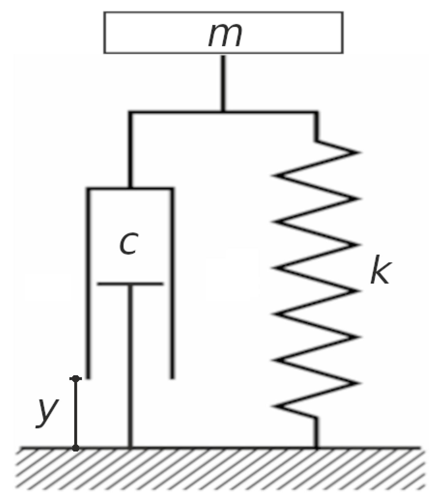
2.1. Dynamic Simulation

In this study, we assume a simplified representation of the dynamic system of an anchored slab experiencing uplift forces by modeling it as a damped unidirectional oscillator, similar to the one shown in Figure 1. The mass can move upwards, pushed by the uplift forces, but it cannot move below the equilibrium position, which corresponds to the ground level at the chute slab location.

Applying the second law of motion to the system of Figure 1, it is obtained that

$${\displaystyle \frac{{\partial }^{2}y}{\partial t^2}}m=LA-g(m-sA{\rho }_{\mathrm{w}})-ky-c{\displaystyle \frac{\partial y}{\partial t}}$$

(3)

where y is the vertical displacement of the slab, taking only positive values ($\mathrm{m}$), L is the pressure given by Equation (2), A is the top view area of the slab (${\mathrm{m}}^2$), m is the mass of the slab ($\mathrm{kg}$), s is the slab thickness ($\mathrm{m}$), k is the spring constant ($\mathrm{N}{\mathrm{m}}^{-1}$), and c is the damping coefficient ($\mathrm{kg}{\mathrm{s}}^{-1}$).

Equation (3) does not include boundary conditions because there is no formula prescribing the dependent variable (displacement) for specific values of the independent variable (time). Instead, it is a piecewise-defined differential equation, where the governing equation depends on the dependent variable. Specifically, Equation (3) applies for $y>0$ and is a second-order, non-homogeneous ordinary differential equation. This type of equation can be solved analytically using the method of variation of parameters [18]. It can also be easily solved by reducing it to a system of first-order ordinary differential equations and then applying a numerical scheme like the Runge–Kutta method [19]. These approaches are typically employed in the case of harmonic oscillators. However, in this case, the domain of acceptable solutions includes only positive vertical displacements. Therefore, to solve Equation (3), we have implemented the following explicit numerical scheme.

$${\displaystyle \frac{y_t-2y_{t-1}+y_{t-2}}{\mathrm{d}{t}^2}}m=L_{t-1}A-g(m-sA{\rho }_{\mathrm{w}})-k{y}_{t-1}-c{\displaystyle \frac{y_t-y_{t-2}}{2\mathrm{d}t}}$$

(4)

The initial conditions for Equation (4) are $y_1=0$ and $y_2=0$. Equation (4) is then solved sequentially to calculate the slab displacement over the time domain. If at any time step t, $y_t<0$, both $y_t$ and $y_{t-1}$ are reset to 0, effectively reapplying the initial conditions. This is because Equation (3) is equivalent to a system of two first-order ordinary differential equations, which requires defining initial conditions for two variables.

The time step $\mathrm{d}t$ should be adequately small to ensure both acceptable accuracy and a detailed description of the dynamics. It should be at most half the natural period of the oscillator, which can be estimated by the following formula [19]:

$$T=2\mathsf{\pi }\sqrt{{\displaystyle \frac{m}{k}}}$$

(5)

2.2. Stochastic Simulation

Fiorotto and Salandin introduced the time interval $\tau$ in their study, defining it as follows: “persistence time $\tau$ is defined as the time interval between an up-crossing and the next down-crossing of a given pressure level” [16]. They showed that persistence time is equally important as the maximum pressure over a time interval in regulating the maximum stress on an anchoring bar. In general, persistence is a characteristic of stochastic processes that exhibit clustering of similar values [20], and is measured with the coefficient $H\in [0,1]$ (the higher the coefficient value, the more persistent the process).

One of the objectives of this study is to investigate the influence of the persistence of the flow velocity on the maximum stress on the anchor bars. Since it is assumed that flow over the spillway is 1D, two alternative univariate stochastic schemes were employed. The first was the AR1 [21,22]:

$$V_t=\mu +a(V_{t-1}-\mu )+b{ϵ}_t$$

(6)

where $V_t$ is the average cross-section velocity at time step t, ${ϵ}_t$ is the innovation or error term, which here follows a Normal Distribution N(0,1), $a={\mathrm{r}}_1$, and $b^2=\gamma (1-a^2)$; $\mu$, $\gamma$, and ${\mathrm{r}}_1$ are the sample mean, variance, and lag-1 autocorrelation, respectively [22].

The second stochastic scheme was the generalized moving average scheme [20]:

$$V_t=\sum _{j=-J}^J{a}_j{ϵ}_t$$

(7)

where J is a large integer, which gives the scale up to which the scheme properly represents the persistence, and the weights $a_j$ are calculate by the following formula:

$$a_j=\sqrt{{\displaystyle \frac{2(1-H)}{{(1.5-H)}^2}}\gamma }\left({0.5|j+1|}^{H+0.5}{+0.5|j-1|}^{H+0.5}-{\left|j\right|}^{H+0.5}\right)$$

(8)

The scale up to which it is important to properly represent persistence is problem-specific. In our case study, J was equal to ${10}^5$.

The first stochastic scheme, given by Equation (6), preserves the mean, variance, and lag-1 autocorrelation, and is suitable for H coefficients around 0.5. The second stochastic scheme, given by Equation (7), preserves the mean, variance, lag-n autocorrelation, and persistence of the observed time series (i.e., the H coefficient). This scheme is suitable for H coefficients approaching 1, i.e., high persistence, and for this reason is also called HK because it is suitable for Hurst–Kolmogorov processes [20]. The synthetic time series produced by both schemes follow a Normal Distribution.

2.3. Case Study

The case study is hypothetical but adopts characteristics that resemble the Oroville Dam. According to the IFT report [4], slab thickness at the location of the failure was 7 inches, i.e., 17.8 $\mathrm{cm}$. The chute design specified No. 11 anchor bars, spaced at 10 feet, i.e., 3.05 $\mathrm{m}$, each way in plan view and extending 5 feet into the foundation (around 1.52 $\mathrm{m}$). This means there was one anchor per slab area of 9.3 ${\mathrm{m}}^2$. The mass of a concrete slab of this area is $9.3{\mathrm{m}}^2\times 0.178\mathrm{m}\times 2320\mathrm{kg}{\mathrm{m}}^{-3}=3840.5\mathrm{kg}$. The elastic modulus of iron is 200 $\mathrm{GPa}$. The No. 11 anchor bar has a cross-section of 1006 ${\mathrm{mm}}^2$. Assuming a bar length equal to 1.52 $\mathrm{m}$, and employing Cook’s uniform bond stress model [23], the spring constant can be calculated equal to $2\times 200\mathrm{GPa}\times 1006{\mathrm{mm}}^2/1.52\mathrm{m}=264.7\mathrm{MN}{\mathrm{m}}^{-1}$. The damping ratio was set equal to 0.06. This is the average ratio reported in the corresponding experiments of Clough (see Table III in [24]) and Sinha et al. (see Figure 7 in [25]).

The oscillations of bodies submerged in fluids are influenced heavily by the reaction forces exerted by the surrounding fluid (water in our case). The most typical approach to represent these forces is to introduce the hydrodynamic mass, which is presumed to be an additional mass to the studied system accounting for the surrounding water reaction forces. For the case of a square submerged plate, the hydrodynamic mass is given by the following formula [25,26]:

$$m_{\mathrm{h}}={\displaystyle \frac{\mathsf{\pi }}{4}}{\rho }_{\mathrm{w}}{l}^3$$

(9)

where l is the length of the side of the square. For the previously mentioned slab characteristics (side equal to 3.05 $\mathrm{m}$), Equation (9) yields $m_{\mathrm{h}}=22,205.7\mathrm{kg}$. This amount is added to the mass of the inertia term, i.e., the mass in the left side of Equations (3) and (4).

The normalized uplift, parameter $\Omega$ in Equation (2), is taken equal to 0.9552, whereas the ratio ${\alpha }^{★}$ in Equation (2) is taken equal to 0.09354. These are the values employed in the example calculation in the Appendix of [7].

The statistical characteristics of the flow are obtained with the following assumptions. The mean velocity is taken equal to the example calculation given in [7], i.e., 30.05 $\mathrm{m}/\mathrm{s}$. The variance is estimated by the turbulence intensity coefficient, which for 1D flows is essentially the coefficient of variation of the velocity magnitude. A plausible and conservative coefficient value equal to 0.1 was assumed (see Figure 16 in [27], Figure 4 in [28], Figure 5 in [29], and Figure 16 in [30]); then, a mean value of 30.05 $\mathrm{m}/\mathrm{s}$ yields a variance equal to ${(30.05\mathrm{m}/\mathrm{s}\times 0.1)}^2=9.03{(\mathrm{m}/\mathrm{s})}^2$. For the HK stochastic scheme, the H coefficient was taken equal to 0.9. We deliberately chose a high value for H to make distinguishable any effect of persistence. Yet, this number is plausible because such high H values have been reported for turbulent flows around jets [31]. The two stochastic schemes produced two synthetic time series that correspond to a time period of 13 h and 53 min.

Regarding the time step of simulation $\mathrm{d}t$, it should be selected fine enough to reliably represent the dynamics of the system. The period of the system, according to Equation (5), is $2\mathsf{\pi }{((m+m_{\mathrm{h}})/k)}^{0.5}=0.062\mathrm{s}$. Therefore $\mathrm{d}t$ should be a fraction of this number. We selected $\mathrm{d}t$ after numerical investigation to ensure minimum overall error in the frequency response curve. Figure 2 displays the amplitude of the oscillations, simulated by Equation (4), for a periodic uplift force generated by a test velocity equal to $30.05\mathrm{m}/\mathrm{s}\times |sin(2\mathsf{\pi }\nu \left)\right|$, where $\nu$ is the frequency of the fluctuation of the test velocity magnitude ranging from 0 to 20 Hz. This figure indicates that the frequency response curves generated from the simulations with time steps 0.001 and 0.0005 $\mathrm{s}$ coincide, which indicates a very small numerical error for time steps finer than 0.001 $\mathrm{s}$.

3. Results

Figure 3 shows the displacement of the hypothetical slab under the ideal scenario of a flow with a constant velocity of 30.05 $\mathrm{m}/\mathrm{s}$, corresponding to the mean value of the case study. The displacement is calculated both with and without accounting for the added hydrodynamic mass to highlight its influence on system response. Including the added mass increases the natural period of the oscillator and reduces the damping effect. In both cases, the oscillation eventually fades to a constant displacement of 0.0012 $\mathrm{m}$, with the maximum displacement reaching approximately 0.0025 $\mathrm{m}$.

Figure 4 displays the histogram of the persistence time $\tau$ of the uplift pressure, i.e., the time interval between the up-crossing and down-crossing of a threshold equal to two times the standard deviation plus the mean. The uplift pressure was calculated from Equation (2) for synthetic time series of velocity generated by AR1 and HK, i.e., Equations (6) and (7). Two histograms are provided in Figure 4, one corresponding to AR1 and one to HK stochastic schemes. The vertical axis gives the frequency—with respect to the total number of exceedance intervals—for $\tau$ measured in simulation time steps. This figure indicates that large persistence times (above 5) are more frequent in the case of the synthetic velocity time series generated with the HK scheme—note: the logarithmic scale is employed for the y-axis; therefore, larger downwards-pointing bars indicate a lower corresponding frequency.

The ratios of the AR1 frequencies to the HK frequencies, as displayed in Figure 4, are 1.04, 0.90, 0.85, 0.88, 1.01, 1.31, 1.36, 1.54, 3.18, and 8.38. This indicates that high uplift pressures (greater than the average plus two times the standard deviation), with durations of 9 and 10 time steps, occur three to eight times more frequently when the driving force—flow velocity—is characterized by high stochastic persistence.

Figure 5 shows the uplift pressure values and the resulting displacement $y_t$ within a 0.2 s window centered around the moment when the maximum simulated $y_t$ occurs for velocities generated using the AR1 and HK schemes. For comparison, this figure also includes the mean uplift pressure and the displacement corresponding to the design uplift pressure (deterministic–static approach). The latter is computed using the formula $A((c_{\mathrm{P}}^{+}+c_{\mathrm{P}}^{-})\overline{L}-sg({\rho }_{\mathrm{c}}-{\rho }_w))/k$, where $\overline{L}$ represents the uplift pressure associated with the mean velocity. The simulation time step used was 0.001 $\mathrm{s}$.

The maximum vertical displacements simulated using synthetic velocities generated by the AR1 and HK schemes were $3.10\times {10}^{-3}$ and $3.38\times {10}^{-3}\mathrm{m}$, respectively. The mean displacement value obtained from both schemes was $1.29\times {10}^{-3}\mathrm{m}$, while the standard deviations were $4.18\times {10}^{-4}$ and $4.32\times {10}^{-4}\mathrm{m}$, respectively, indicating similar values. The simulated displacements for the AR1 and HK schemes exceeded a threshold value, defined as the mean plus four times the standard deviation, 25 and 396 times, respectively (note that $396/25\approx 15$).

To evaluate the impact of the time step, simulations were repeated with a time step of $0.0005\mathrm{s}$, while doubling the length of the synthetic time series for velocity to ensure an equivalent simulation period to the time step of $0.001\mathrm{s}$. The maximum vertical displacements simulated using synthetic velocities produced by the AR1 and HK schemes were $2.6437\times {10}^{-3}$ and $3.2971\times {10}^{-3}\mathrm{m}$, respectively. Comparing these values with those obtained using a time step of $0.001\mathrm{s}$, it can be inferred that the maximum displacement in simulations based on the synthetic time series employing the AR1 scheme was significantly reduced.

4. Discussion

The simulation results indicate that both the stochastic properties of the flow velocity (such as variance and persistence) and the characteristics of the bar–slab oscillator significantly affect the maximum stress exerted on the anchoring bar of a chute slab. The discussion of the results is as follows:

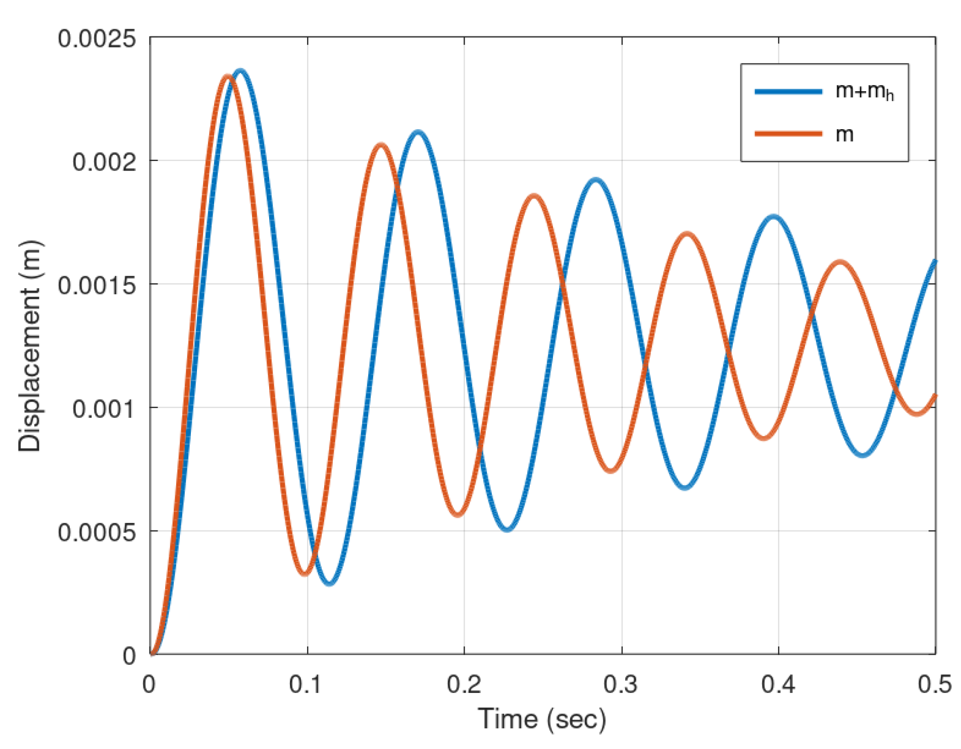
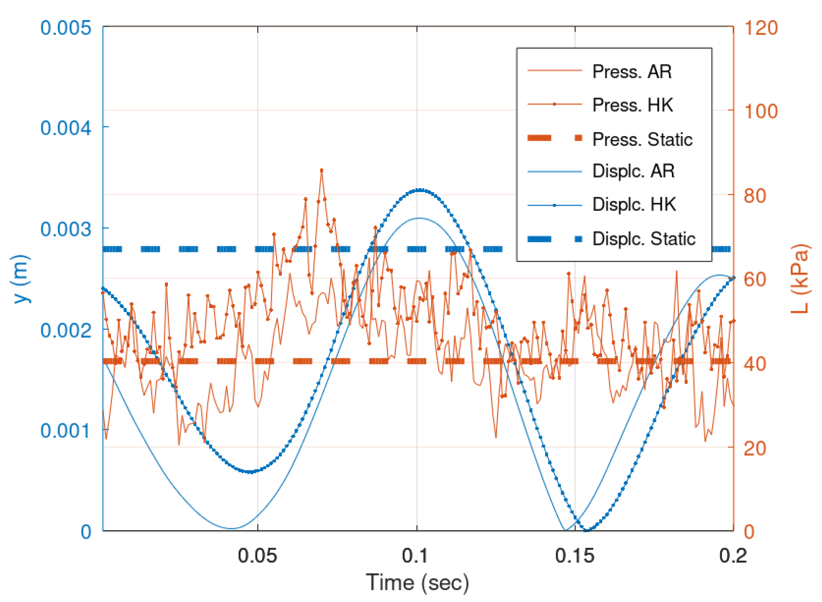
• The deterministic–static method may underestimate the maximum stress on an anchoring bar. In our case study, the stochastic–dynamic approach resulted in 9% to 19% higher maximum displacement, depending on the stochastic persistence of the velocity. For the case study’s mean velocity of 30.05 m/s, the summation of positive and negative pressure coefficients obtained from the synthetic velocity time series is $c_{\mathrm{P}}^{+}+c_{\mathrm{P}}^{-}=(max{\left(V_t\right)}^2-min{\left(V_t\right)}^2)/\mathrm{mean}{\left(V_t\right)}^2\approx 2$, similar to the value suggested in [9]. Consequently, the maximum expected uplift pressure is 80 kPa, closely matching the maximum value observed in the stochastic–dynamic approach shown in Figure 5. However, the maximum displacement according to the deterministic–static approach is 2.83 mm, whereas the stochastic–dynamic approach yielded maximum displacements of 3.10 mm and 3.38 mm for synthetic velocity time series generated using AR1 and HK, respectively. This underscores the significance of considering the dynamic behavior of the slab–anchoring bar system.
• Under typical conditions, the stochastic persistence plays a significant role in determining the maximum stress on chute slabs. Specifically, the maximum displacement calculated in the case study using synthetic time series of velocities with a Hurst–Kolmogorov (HK) model was 9% higher than that calculated using an autoregressive model of order 1 (AR1). This result is consistent with the findings of Fiorotto and Salandin [16], who highlighted the importance of persistence times, defined as the number of consecutive exceedances of uplift pressure. However, our study adopts a more generalized approach, treating persistence as an inherent property of the stochastic structure of flow velocity, which is the primary driving force behind the stresses on the chute slab.
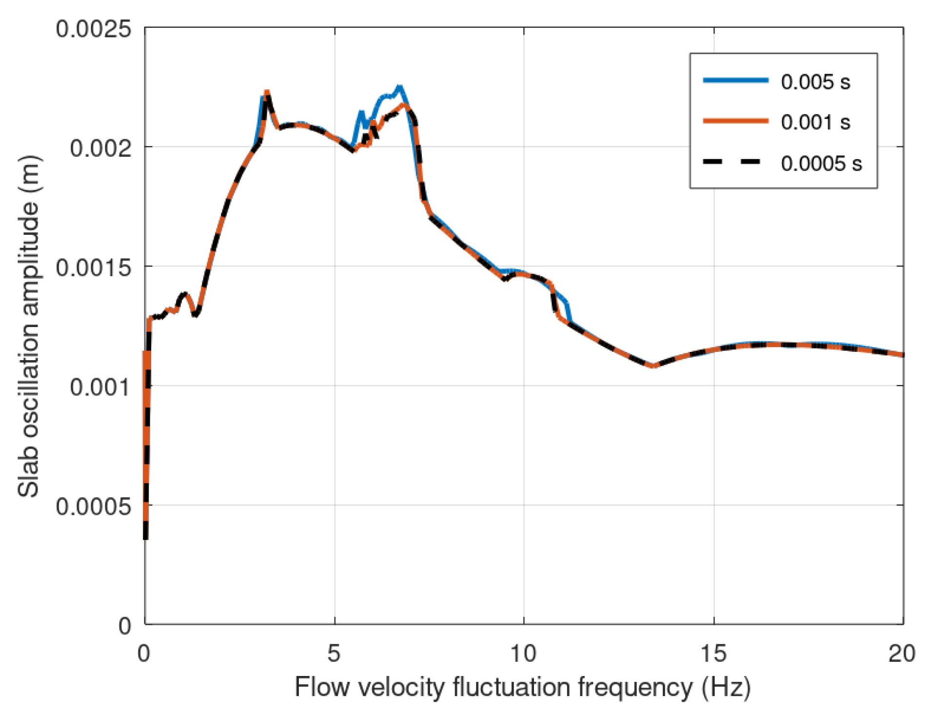
• The simulation time step must be carefully chosen to ensure that numerical errors remain within acceptable tolerance limits. In our case study, which, although hypothetical, is based on typical characteristics, the time step needed to be finer than $0.005\mathrm{s}$. Consequently, simulations were performed with time steps of $0.001\mathrm{s}$ and $0.0005\mathrm{s}$. At these time scales, the variance of the flow velocity was assumed to be constant. As a result, the stress indices (i.e., the displacements) for the $0.0005\mathrm{s}$ time step were lower compared to those for the $0.001\mathrm{s}$ time step due to the proportionally shorter interval duration $\tau$ for smaller time steps. This effect is more evident in the case of AR1. This discrepancy is attributed to the fact that AR1, suitable for Markovian processes, produces a much steeper climacogram compared to Hurst–Kolmogorov processes. In contrast, Hurst–Kolmogorov processes, with their less steep climacogram, exhibit smaller deviations under the same assumption [20]. This further highlights the importance of selecting the most appropriate stochastic scheme for analysing stochastic process that drive dynamic systems.

The impact of vertical displacement on the disturbance of the flow was not accounted for in the simulations. Typically, vertical displacement is expected to increase the coefficient $\Omega$ in Equation (2), resulting in higher uplift pressures (L) for the same flow velocity. The value of 0.9552 used in our simulations corresponds to a ratio of joint gap to slab vertical offset of 12.7/12.7 mm/mm = 1 [7]. The maximum simulated slab displacement is 3.5 mm (Figure 5), which reduces the ratio to 0.78. However, the normalized uplift $\Omega$ increases non-linearly and slowly with a decreasing ratio (see Figure 7 in [7]), and the value is already very close to the upper limit of $\Omega$, which is 1. Therefore, the positive feedback is negligible in our case study.

It should be noted that the reported displacement values are based on a specific length of the generated synthetic time series, which for this case study corresponds to a duration of 13 h and 53 min. This choice of length introduces some subjectivity into the analysis. To address this subjectivity, a comprehensive probabilistic approach should be employed [32,33]. This involves generating time series of sufficient length—multiple times the duration of any plausible dangerous event—to produce reliable return period plots. Subsequently, the maximum stresses can be assessed based on an acceptable level of probability of exceedance as defined by the design study.

In this case study, plausible statistical parameters were assumed for the AR1 and HK stochastic simulation schemes. However, in real applications, these parameters should be derived from measurements. This can pose a challenge if preliminary numerical analysis suggests the need for a very small time step. Nevertheless, Bellin and Fiorotto state that “analysis of force power spectrum suggests that the fluctuation energy is mainly concentrated at the lower end of the spectrum” (see also Figure 3 in [9]). Furthermore, later studies indicate that variance stabilizes below a certain scale [34], which aligns with a fundamental physical principle: a continuously increasing variance at lower scales would imply infinite variance at infinitesimal scales, requiring infinite energy to manifest [20]. Therefore, a measurement frequency of a few hundred Hz should be sufficient to capture the necessary information for a stochastic scheme suited to turbulent flow processes, such as the filtered Hurst–Kolmogorov family [20,34].

It is essential to highlight that the maximum displacement—and consequently the maximum stress—shown in Figure 5 is not directly caused by the maximum uplift pressure. For the AR1 model, the maximum displacement occurs at $t=586.49\mathrm{s}$, whereas the maximum uplift pressure occurs at $t=600.20\mathrm{s}$, i.e., $13.71\mathrm{s}$ later. For the HK model, the maximum displacement occurs at $t=118.67\mathrm{s}$, while the maximum uplift pressure occurs at $t=109.15\mathrm{s}$, i.e., $9.52\mathrm{s}$ earlier. Given that Figure 5 covers only a $0.2\mathrm{s}$ time window—well separated from the occurrence of maximum pressures—it is clear that uplift pressure alone does not dictate maximum stress. This highlights the critical role of the stochastic structure, particularly persistence, in shaping stress dynamics. While this study provides valuable insights into the role of persistence in shaping maximum stress, it is important to acknowledge its limitations. The absence of direct stress measurements means that the findings rely on numerical modeling rather than empirical validation. Future research should prioritize experimental investigations to measure anchoring bar stresses directly, thereby improving the validation of the stochastic–dynamic approach and refining our understanding of structural responses under stochastic hydraulic conditions.

Two important aspects not examined in this study are the stress on the anchoring bar and the effects of creep. Creep occurs under sustained extreme loading conditions, while stress analysis on the anchoring bar could initially be approached using Hooke’s law—multiplying displacement by the spring constant and dividing by the bar’s cross-sectional area. However, this approach is overly simplistic. In the uniform bond stress model, the anchoring force is distributed uniformly along the bonded anchor’s curved surface area, making Hooke’s law insufficient for accuracy. Moreover, the stress–displacement proportionality holds only within the elastic region. As for creep, a common failure mechanism, it results from prolonged exposure to extreme stress (see Figure 1 in [35]), highlighting its dependence on the duration of elevated stress values, and hence on persistence. A more detailed modeling of the anchoring bar is needed to provide reliable predictions regarding material and anchoring failure.

When acquiring measurements, two key issues need to be considered. The first concerns the scale of physical models, often used to study hydraulic structures in laboratories, as there is evidence that it unpredictably influences persistence. Nordin et al. [36] reported findings on turbulent flows, showing that for flow depths of 1.4 cm, 28 cm, 3.4 m, and 10.7 m, the corresponding H values were 0.60, 0.84, 0.93, and 0.95, respectively. This trend suggests that the characteristic length of a flow may influence its persistence. Therefore, if a scale model is used, it is questionable whether the resulting measurements will accurately represent the persistence of the full-scale flow.

Measurements, whether from laboratory experiments or real-world observations, are subject to inherent biases, especially when dealing with stochastic processes that exhibit high persistence. Statistical estimators for these processes tend to underestimate values, leading to increased bias. For example, the expected value $\widehat{\gamma }$ of the typical variance estimator (the expected value is necessary since a statistical estimator is itself a random variable) underestimates the actual variance $\gamma$ when only n measurements are available, as shown by the following formula [20]:

$$\widehat{\gamma }=(1-{\displaystyle \frac{1}{n^{2-2H}}})\gamma$$

(10)

A numerical investigation using Equation (10) indicates that for a limited number of measurements and high persistence, the underestimate may be significant. For instance, with 1000 measurements and a coefficient H of 0.9, the variance estimator underestimates the true variance by 25%.

A point of debate arises regarding the specifications of the unidirectional oscillator. The added hydrodynamic mass, as calculated by Equation (9), typically applies to a fully submerged square plate. However, spillway slabs only contact flowing water on their upper surface, while the lower surface remains dry or, in cases of water infiltration, in contact with a thin film of water that may contribute to uplift pressure. One might argue that the mass of this thin film is negligible, suggesting that the right-hand side of Equation (9) be halved. Conversely, it could also be reasoned that the rapid and small displacements of the slabs justify using the equation as is, even with a millimeter-thin water film. This issue requires further investigation.

The development of uplift forces is a complex, multi-stage process, with each stage marked by significant uncertainty. While stagnation pressure at the obstacle level—corresponding to the offset of a chute slab—can be calculated straightforwardly from flow velocity, the full development of uplift forces involves more intricate mechanisms. In this study, these mechanisms were represented using simplified approaches applicable to specific cases, such as assuming instantaneous pressure propagation under the slab and a small integral scale relative to slab length [11]. Given the stochastic–dynamic nature of the system, the intermediate calculation stages between flow velocity and uplift force require additional exploration through targeted hydraulic experiments.

5. Conclusions

This study examined the impact of the stochastic characteristics of flow velocity on the stresses exerted on spillway components. A stochastic simulation of flow velocity was combined with a dynamic simulation of an anchoring bar–slab system, forming a stochastic–dynamic approach. The findings demonstrate that the stochastic characteristics of flow velocity, as the driving force, play a crucial role in the system’s behavior, indicating that deterministic methods may not be adequate for thoroughly studying these types of problem. The hypothetical case study, which mimics the hydraulic characteristics of the Oroville Dam spillway incident, revealed that the deterministic method underestimated the stresses on anchoring bars by 19%. Other important findings from the study include the following:

• While deterministic models can offer rough estimates, they may overlook critical stress factors introduced by random fluctuations in flow velocity. The persistence of the magnitude of flow velocity significantly impacts the maximum stress developed on the anchoring bar. The duration of extreme conditions is also influenced by this persistence, which in turn controls creep and likely the rate of overall structural degradation.
• Various researchers have conducted experiments to obtain velocity and pressure measurements in turbulent flows. However, this study, which focuses on the maximum stress of anchoring bars, highlights that such datasets provide minimal support for studying maximum stress. This is because, as found in this study, maximum stress is not directly related to maximum pressure, and the persistence of velocity in physical models does not necessarily match that of real-world systems, as suggested by previous studies.
• In the stochastic–dynamic approach, accurately representing the system’s response requires selecting an appropriate simulation time step. However, finer time steps demand higher-frequency observations, which may not always be feasible. In such cases, disaggregation of available measurements using suitable stochastic models (e.g., filtered Hurst–Kolmogorov) may be necessary to generate input time series for the dynamic system at the required temporal scale.

Since no experimental data are available for the maximum stress on the anchoring bars, future experiments measuring these stresses would greatly enhance our understanding of the underlying processes and provide critical validation of the proposed approach. Additionally, future research should focus on refining the stochastic–dynamic approach and improving measurement techniques to maintain accuracy at higher temporal resolutions. Such efforts will advance our understanding of structural safety under stochastic hydraulic conditions and help mitigate the risk of spillway failures.

References

1. Boelens, R.; Shah, E.; Bruins, B. Contested Knowledges: Large Dams and Mega-Hydraulic Development. Water 2019, 11, 416. [Google Scholar] [CrossRef]
2. Song, J.; Sciubba, M.; Kam, J. Risk and Impact Assessment of Dams in the Contiguous United States Using the 2018 National Inventory of Dams Database. Water 2021, 13, 1066. [Google Scholar] [CrossRef]
3. Ageing Dams Pose Growing Threat. 2024. Available online: https://unu.edu/press-release/ageing-dams-pose-growing-threat (accessed on 23 September 2024).
4. France, J.W.; Alvi, I.A.; Dickson, P.A.; Falvey, H.T.; Rigbey, S.; Trojanowski, J. Independent Forensic Team Report: Oroville Dam Spillway Incident. 2018. Available online: https://damsafety.org/sites/default/files/files/Independent%20Forensic%20Team%20Report%20Final%2001-05-18.pdf (accessed on 6 June 2024).
5. Koskinas, A.; Tegos, A.; Tsira, P.; Dimitriadis, P.; Iliopoulou, T.; Papanicolaou, P.; Koutsoyiannis, D.; Williamson, T. Insights into the Oroville Dam 2017 Spillway Incident. Geosciences 2019, 9, 37. [Google Scholar] [CrossRef]
6. Frizell, K. Uplift and Crack Flow Resulting from High Velocity Discharges over Open Offset Joints; U.S. Department of the Interior Bureau of Reclamation, Technical Service Center: Denver, CO, USA, 2007. [Google Scholar]
7. Wahl, T.L.; Heiner, B.J. Laboratory Measurements of Hydraulic Jacking Uplift Pressure at Offset Joints and Cracks. J. Hydraul. Eng. 2024, 150, 04024016. [Google Scholar] [CrossRef]
8. Te Chow, V. Open Channel Hydraulics; McGraw-Hill: New York, NY, USA, 1959; pp. 28–29. [Google Scholar]
9. Bellin, A.; Fiorotto, V. Direct dynamic force measurement on slabs in spillway stilling basins. J. Hydraul. Eng. 1995, 121, 686–693. [Google Scholar] [CrossRef]
10. Toso, J.W.; Bowers, C.E. Extreme Pressures in Hydraulic-Jump Stilling Basins. J. Hydraul. Eng. 1988, 114, 829–843. [Google Scholar] [CrossRef]
11. Fiorotto, V.; Rinaldo, A. Fluctuating uplift and lining design in spillway stilling basins. J. Hydraul. Eng. 1992, 118, 578–596. [Google Scholar] [CrossRef]
12. The Comprehensive Manual for Velocimeters Vector | Vectrino | Vectrino Profiler; NORTEK AS: Rud, Norway, 2018.
13. Shumway, R.H.; Stoffer, D.S. Time Series Analysis and Its Applications; Springer: Cham, Switzerland, 2017. [Google Scholar]
14. Liew, J.R.; Shanmugam, N.; Yu, C. Structural Analysis. In Structural Engineering Handbook; Wai-Fah, C., Ed.; CRC Press LLC: New York, NY, USA, 1999. [Google Scholar]
15. Gardner, M.; Sitar, N. Modeling of Dynamic Rock–Fluid Interaction Using Coupled 3-D Discrete Element and Lattice Boltzmann Methods. Rock Mech. Rock Eng. 2019, 52, 5161–5180. [Google Scholar] [CrossRef]
16. Fiorotto, V.; Salandin, P. Design of Anchored Slabs in Spillway Stilling Basins. J. Hydraul. Eng. 2000, 126, 502–512. [Google Scholar] [CrossRef]
17. Barjastehmaleki, S.; Fiorotto, V.; Caroni, E. Design of Stilling Basin Linings with Sealed and Unsealed Joints. J. Hydraul. Eng. 2016, 142, 04016064. [Google Scholar] [CrossRef]
18. Pierce, R. The Method of Variation of Parameters. 2024. Available online: https://www.mathsisfun.com/calculus/differential-equations-variation-parameters.html (accessed on 22 July 2024).
19. Harihara, P.; Childs, D.W. Solving Problems in Dynamics and Vibrations Using MATLAB; Department of Mechanical Engineering Texas A & M University: College Station, TX, USA, 2014; pp. 11–21. [Google Scholar]
20. Koutsoyiannis, D. Stochastics of Hydroclimatic Extremes—A Cool Look at Risk, 3rd ed.; KALLIPOS: Athens, Greece, 2023. [Google Scholar]
21. Matalas, N.; Wallis, J. Generation of synthetic flow sequences. In Systems Approach to Water Management; Biswas, A., Ed.; McGraw-Hill: New York, NY, USA, 1976. [Google Scholar]
22. Salas, J.D. Chap. 19: Analysis and modelling of hydrological time series. In Handbook of Hydrology; Maidment, D., Ed.; McGraw-Hill: New York, NY, USA, 1993; Volume 19. [Google Scholar]
23. Cook, R.A.; Kunz, J.; Fuchs, W.; Konz, R.C. Behavior and design of single adhesive anchors under tensile load in uncracked concrete. ACI Struct. J. 1998, 95, 9–26. [Google Scholar]
24. Clough, R.W. Effects of Earthquakes on Under-Water Structures. In Proceedings of the 2nd World Conference on Earthquake Engineering, Tokyo, Japan, 11–18 July I960.
25. Sinha, J.K.; Singh, S.; Rama Rao, A. Added mass and damping of submerged perforated plates. J. Sound Vib. 2003, 260, 549–564. [Google Scholar] [CrossRef]
26. Dong, R. Effective Mass and Damping of Submerged Structures; Technical Report; Lawrence Livermore National Lab. (LLNL): Livermore, CA, USA, 1978. [Google Scholar]
27. Jafari, R.; Sui, J. Velocity Field and Turbulence Structure around Spur Dikes with Different Angles of Orientation under Ice Covered Flow Conditions. Water 2021, 13, 1844. [Google Scholar] [CrossRef]
28. Chanson, H.; Carosi, G. Turbulent time and length scale measurements in high-velocity open channel flows. Exp. Fluids 2007, 42, 385–401. [Google Scholar] [CrossRef]
29. Kim, H.S.; Choi, S.; Park, M.; Ryu, Y. Flow Turbulence and Pressure Fluctuations in a Hydraulic Jump. Sustainability 2023, 15, 14246. [Google Scholar] [CrossRef]
30. Chowdhury, S.; Sen, D.; Dey, S. Submerged wall jet on a macro-rough boundary: Turbulent flow characteristics and their scaling laws. Environ. Fluid Mech. 2024, 24, 587–610. [Google Scholar] [CrossRef]
31. Dimitriadis, P.; Papanicolaou, P. Statistical analysis of positively buoyant turbulent jets. In Proceedings of the European Geosciences Union General Assembly 2012, EGU General Assembly, Vienna, Austria, 22–27 April 2012. [Google Scholar]
32. Rozos, E.; Leandro, J.; Koutsoyiannis, D. Stochastic Analysis and Modeling of Velocity Observations in Turbulent Flows. J. Environ. Earth Sci. 2024, 6, 4–56. [Google Scholar] [CrossRef]
33. Rozos, E.; Wieland, J.; Leandro, J. Measuring Turbulent Flows: Analyzing a Stochastic Process with Stochastic Tools. Fluids 2024, 9, 128. [Google Scholar] [CrossRef]
34. Dimitriadis, P.; Koutsoyiannis, D.; Papanicolaou, P. Stochastic similarities between the microscale of turbulence and hydro-meteorological processes. Hydrol. Sci. J. 2016, 61, 1623–1640. [Google Scholar] [CrossRef]
35. Kränkel, T.; Lowke, D.; Gehlen, C. Prediction of the creep behaviour of bonded anchors until failure—A rheological approach. Constr. Build. Mater. 2015, 75, 458–464. [Google Scholar] [CrossRef]
36. Nordin, C.F.; McQuivey, R.S.; Mejia, J.M. Hurst phenomenon in turbulence. Water Resour. Res. 1972, 8, 1480–1486. [Google Scholar] [CrossRef]
Figure 1. Unidirectional oscillator of a mass, a spring, and a damper.
Water 17 00621 g001
Figure 2. Resonance curve obtained from simulations with time steps of 0.005, 0.001, and 0.0005 s . Note: the maximum allowable strain for iron is not considered.
Water 17 00621 g002
Figure 3. Displacement for constant flow velocity V = 30.05   m / s , with and without the added hydrodynamic mass m h . Note: the maximum allowable strain for iron is not considered.
Water 17 00621 g003
Figure 4. Histogram of the persistence time of the synthetic flow velocity produced with (a) AR1 and (b) HK.
Water 17 00621 g004
Figure 5. The synthetic uplift pressure values ( L t ) and resulting displacement ( y t ) for velocity time series produced with AR1 and HK. The blue and orange horizontal lines indicate the maximum displacement obtained with the conventional (deterministic–static) approach and the uplift pressure corresponding to a constant velocity equal to the mean value ( L ¯ ).
Water 17 00621 g005
Disclaimer/Publisher’s Note: The statements, opinions and data contained in all publications are solely those of the individual author(s) and contributor(s) and not of MDPI and/or the editor(s). MDPI and/or the editor(s) disclaim responsibility for any injury to people or property resulting from any ideas, methods, instructions or products referred to in the content.