Ecological Health Assessment of Karst Plateau Wetlands Based on Landscape Pattern Analysis

Abstract

This study analyzed the changes in landscape patterns and the ecological health status of karst plateau wetlands, providing valuable insights into their conservation. Using land cover data from 1996 to 2021, DEM, and Landsat series satellite imagery, this study employed landscape ecology methods and the pressure–state–response (PSR) model framework. A regional landscape grid was constructed, and 13 indicators were selected to establish an ecological health evaluation system for karst plateau wetlands. This allowed us to explore the spatiotemporal change characteristics of the landscape pattern and the ecological health of karst plateau wetlands. The results showed that over a 25-year period, farmland, grassland, and construction land areas have increased, whereas forested land areas have decreased. Water bodies remained relatively stable but showed a trend of transitioning into grassland. Unused land showed no significant change. Landscape analysis indicated that grasslands experience the highest rate of fragmentation, complex shapes, and greater heterogeneity, whereas water bodies have the lowest fragmentation, more regular shapes, and lower heterogeneity. Other landscape types exhibited moderate characteristics. Overall, the landscape of the study area exhibited high fragmentation, specific patch aggregation, moderate patch density, and low diversity. A comprehensive ecological health evaluation revealed that the wetland health value remained at an “unhealthy” level from 1996 to 2021. Although there was a brief improvement in 2010, effective long-term recovery was not achieved. Spatially, the proportion of “diseased” areas peaked in 2006, and most grid zones remained in an “unhealthy” state over the years, with none reaching the “healthy” standard. These findings highlight the severe challenges faced by the wetland ecosystem.

1. Introduction

Wetlands, one of Earth’s critical ecosystems, are widely distributed across various environments, from polar regions to tropical zones. Common wetland types include riverine, lacustrine, coastal, marsh, artificial, and unique karst plateau wetlands. These diverse habitats play pivotal roles in climate regulation, water purification, and biodiversity conservation [1,2,3]. Karst plateau wetlands are notable because of their distinctive geological structures and hydrological conditions, which form a complex ecosystem. Karst plateau wetlands develop on limestone or dolomite foundations, where intense dissolution processes shape landscapes characterized by stone forests, caves, and subterranean rivers. This peculiar geology creates an intricate and dynamic interaction between the surface and groundwater systems, leading to significant seasonal fluctuations in water levels and volumes [4]. Plant communities exhibit remarkable adaptability to alternating periods of dryness and moisture, with some species being endemic or specially adapted to extreme environmental conditions [5]. Moreover, these wetlands are vital for water retention, maintaining regional water balance, and providing habitats for numerous flora and fauna, thereby safeguarding biodiversity. However, alongside population growth and economic development, human activities are increasingly disturbing these sensitive areas, resulting in reduced wetland coverage, deteriorating water quality, and declining biodiversity [6]. Therefore, assessing the ecological health of karst plateau wetlands is crucial for effective natural resource management and conservation from both a scientific and ecological preservation perspective. Precise evaluation methods are essential for monitoring the state of karst plateau wetlands. Such efforts are not only fundamental for understanding these ecosystems but also indispensable for guiding sustainable practices that ensure longevity and functionality within the broader landscape of nature’s interconnected web of life.

Thus, the accurate evaluation of wetland ecological health is pivotal for effective natural resource management and conservation. The assessment of wetland health has evolved since the early 20th century [7,8], with Larson’s 1972 model marking a milestone as the first rapid assessment tool for wetland functions [9]. Initially, assessments were largely based on singular physical, chemical, or biological indicators [10], but since the 1990s, they have transitioned towards more comprehensive multiparameter approaches. These include frameworks such as the pressure–state–response (PSR) model [11,12], landscape ecology methodologies [13,14], integrated assessment models [15,16], and multivariate statistical analyses [17], all of which aim to capture the intricate nature of wetland ecosystems. Rapport (1992) [18] introduced a tripartite classification of biological, physical, and socioeconomic indicators to evaluate wetland health by applying this framework to riverine wetlands. The Hydrogeomorphic (HGM) Method, developed by Brooks et al. [19] and refined by Gebo and Brooks [20], provides a landscape-scale assessment framework for wetland functions through hydrogeomorphic classification analysis. Liu et al. [21] developed a 13-indicator system encompassing the water environment, surface sediments, biota, landscape, and societal dimensions to assess Wuhan’s Lake wetlands. Advances in remote sensing and Geographic Information Systems (GISs) have enabled large-scale dynamic monitoring, significantly enhancing the precision and timeliness of evaluations [22]. For instance, Wang et al. [23] constructed an operational assessment indicator system for wetland ecosystem health by integrating functional characteristics, ecological features, and social environmental factors, with 3S technology serving as the core technical approach. Despite extensive research on wetland health, studies on karst plateau wetlands remain limited, particularly those integrating multiple landscape elements for systematic ecological health assessments. Landscape pattern analysis is a powerful approach for quantifying distribution patterns, patch shape complexity, and spatial associations within wetlands. It reveals how internal structures change and respond to external disturbances. This method identifies key areas and trends in ecological processes and provides a scientific basis for targeted conservation strategies.

Considering the unique advantages of landscape pattern analysis in elucidating wetland structure and assessing ecological health, this study focuses on karst plateau wetlands, using the Caohai National Nature Reserve in Guizhou as a case study. By adopting a landscape ecology perspective and combining landscape pattern analysis with the PSR model framework, we developed an evaluation system tailored to karst plateau wetlands. This approach enhances our understanding of these distinctive wetland ecosystems and provides valuable insights into their conservation, contributing to a broader field of environmental science.

2. Materials and Methods

2.1. Study Area

Nestled in the heart of the Wumeng Mountains at the apex of the central Yungui Plateau, the Caohai National Nature Reserve is situated southwest of Weining County, within the multi-ethnic Weining Yi, Hui, and Miao Autonomous County, Guizhou Province, China. The reserve spans a geographic range of 26°47′32″–26°52′32″ N latitude and 104°10′16″–104°20′40″ E longitude (Figure 1) [24]. It belongs to the Yangtze River watershed and encompasses the largest natural plateau freshwater lake in Guizhou. As a typical karst lake, it serves as a prime example of a subtropical plateau wetland ecosystem in China [25,26]. The reserve is predominantly characterized by yellow-brown soil, with an annual average temperature of 10.6 °C and a mean annual precipitation of 950.9 mm. The region receives ample sunshine, with an average annual insolation value of 1805.4 h, making it one of the sunniest places in Guizhou [27].

2.2. Data Sources

The primary datasets utilized in this study included land cover data, digital elevation model (DEM) data, and satellite remote sensing imagery from Landsat 5 TM and Landsat 8 OLI. Remote sensing and DEM data were primarily sourced from the Geospatial Data Cloud (https://www.gscloud.cn, accessed on 10 January 2025). Land cover data, covering the period from 1985 to 2021 at a resolution of 30 m, were provided by Professor Huang Xin’s team at the Institute of Remote Sensing Information Processing, Wuhan University (http://irsip.whu.edu.cn/, accessed on 10 January 2025) [28]. Considering data availability, we selected land use and remote sensing data from 1996, 2000, 2006, 2010, 2018, and 2021 as the primary data sources. Initially, the land cover data were categorized into cropland, forests, shrubland, grassland, water bodies, barren land, and impervious surfaces. After comparing these classifications with contemporary, regional remote sensing data and considering the specific conditions of the study area, the land cover types were reclassified into cropland, forests (including forests and shrubland), grassland, water bodies, unused land (barren land), and built-up areas. The DEM data were processed using ArcMap 10.8 to extract slope information through clipping and slope calculations. Vegetation cover data were derived from six phases of satellite remote sensing images using ENVI 5.3 software, which involved radiometric calibration, atmospheric correction, and band calculations.

2.3. Methods

2.3.1. Selection and Calculation of Landscape Index

To thoroughly investigate the evolving characteristics of the landscape pattern in the study area, we engaged in discussions at both the patch type and landscape levels. To ensure the comprehensiveness, feasibility, and scientific rigor of the selected indicators, we drew upon previous research to establish the following main criteria for selecting landscape indicators [13,29,30]: (1) Scientific Rationality: the indicators should be grounded in landscape ecology theory and capable of effectively measuring the size, distribution, and connectivity of wetland patches. (2) Representativeness and Independence: the selected indicators must comprehensively reflect key aspects of landscape structure, function, and dynamic changes, such as diversity, connectivity, and fragmentation while maintaining a degree of independence from one another. (3) Interpretability and Transparency: the indicators should be straightforward to explain and understand, facilitating communication with other researchers and decision-makers. (4) Sensitivity and Responsiveness: the indicators must be sufficiently sensitive to environmental changes (e.g., human activities, climate change) and should timely reflect alterations in landscape structure and function while also maintaining stability and consistency over time for trend analysis. (5) Empirical Validation: the indicators should be documented in relevant studies to ensure they are widely accepted and validated, thus providing a solid scientific foundation. Based on these criteria, at the patch-type level, we selected the patch area (CA), percentage of landscape (PLAND), largest patch index (LPI), and number of patches (NPs) to characterize the dominance of various landscape types and their changes. Additionally, we chose the aggregation index (AI), mean patch size (MPS), patch density (PD), and landscape shape index (LSI) to assess the degree of fragmentation of the wetland landscape. At the landscape level, the landscape division index (DIVISION), aggregation index (AI), Shannon evenness index (SHEI), Shannon diversity index (SHDI), patch density (PD), and contagion index (CONTAG) were selected for evaluation to explore landscape change. The ecological significance represented by these indices is shown in

Table 1. Landscape pattern index and ecological significance.

Landscape Pattern Index	Ecological Significance
Patch Area (CA)	Measures the total area covered by a specific type of landscape patch. It helps identify the most extensive patches and their contribution to the overall landscape structure.
Percentage of Landscape (PLAND)	Indicates the proportion of the entire landscape occupied by each type of patch. This metric is crucial for understanding the relative abundance of different land cover types over time.
Largest Patch Index (LPI)	Reflects the largest contribution of a single patch to the total area of a particular landscape type. LPI is an important indicator of landscape connectivity and fragmentation.
Number of Patches (NP)	Counts the number of individual patches of a certain type within the study area. NP provides information on the degree of fragmentation or aggregation of a given landscape type.
Aggregation Index (AI)	Measures the degree to which similar patches are clustered together. AI is essential for evaluating landscape connectivity and the potential for species movement across the landscape.
Mean Patch Size (MPS)	Mean patch size (MPS) reflects the overall size characteristics of patches within a landscape and aids in understanding the spatial structure and function of the landscape.
Patch Density (PD)	Counts the number of patches per unit area, indicating the level of landscape fragmentation. PD is vital for understanding habitat availability and fragmentation impacts.
Landscape Shape Index (LSI)	The landscape shape index (LSI) quantifies the complexity of patch boundaries, reflecting the irregularity of patch shapes and their sensitivity to ecological functions and human impacts.
Landscape Division Index (DIVISION)	Quantifies the extent to which the landscape has been divided into smaller patches. Higher values indicate greater fragmentation, often associated with increased human activity.
Shannon Evenness Index (SHEI)	Evaluate the evenness of landscape-type distribution. SHEI helps understand the balance between different landscape elements and can signal environmental stress or stability.
Shannon Diversity Index (SHDI)	Assesses the diversity of landscape types within the study area. SHDI is a fundamental metric for biodiversity conservation and ecosystem management.
Contagion Index (CONTAG)	Measures the tendency of patches to be adjacent to other patches of the same type. CONTAG reflects the spatial arrangement of landscape elements and can influence ecological interactions and processes.

[31].

2.3.2. Construction of a Wetland Landscape Ecological Health Diagnostic System

Wetlands are complex ecosystems, and their ecological health cannot be adequately assessed using a single evaluation metric. Therefore, this study builds on landscape ecology principles by drawing from previous frameworks for wetland [32,33,34,35,36] and mountain landscape ecological health assessments [37]. Adhering to the principles of scientific rigor, uniqueness, comprehensiveness, and practicality, we developed a diagnostic system considering the environmental context of karst plateau wetlands. To achieve this, we established a 0.3 km × 0.3 km landscape grid, allowing for detailed ecological health diagnostics within each grid cell across the study area. Using the PSR model framework, we selected 13 indicators encompassing pressure, state, and response (

Table 2. Landscape health karst plateau wetland ecosystem health evaluation index system level.

Objective Layer	Principle Level	Quota Level
Ecological health assessment of wetlands	Pressure	Slope X1
		Comprehensive index of land use degree X2
		Human interference index X3
	State	Shannon’s diversity index X4
		Shannon’s evenness index X5
		Patch richness X6
		Mean patch size X7
		Hydrological regulation index X8
		Vegetation coverage X9
		Landscape division index X10
	Response	Landscape restoration index X11
		ESV X12
		Aggregation index X13

) to construct a robust ecological health assessment system specifically tailored for karst plateau wetlands. This approach ensured a thorough and nuanced understanding of the ecological dynamics within these unique wetland environments, providing a solid foundation for conservation and management efforts.

Pressure Indicators: Located near the urban area of Weining County, the Caohai Wetland Nature Reserve has undergone on-site investigations, revealing that human activities constitute the primary source of pressure on this delicate ecosystem. To reflect the sources of pressure on wetlands, considering the availability and representativeness of the data, we selected the slope, an integrated index of land use intensity, and an index of anthropogenic disturbance as indicators. The slope data were derived from the SRTM DEM, with calculations performed using ArcMap 10.8, yielding a resolution of 30 m.

The integrated index of land use intensity [38] reflects the extent and intensity of land use based on the cumulative outcome of various transformations in land use types. The classification index was set at one for unused land; two for forests, grasslands, and water bodies; three for cultivated land; and four for constructed land (the highest index). The index is calculated as follows:

$$A=100\times {\sum }_i^n\left(P_i\times S_i\right)$$

(1)

where $A$ represents the integrated index of land-use intensity, with a range of $A\in [100, 400]$; $P_i$ denotes the classification index for the $i$-th level of land use; $S_i$ signifies the proportion of the area covered by the $i$-th level of land use; and $n$ indicates the total number of land use categories.

The human disturbance index (HDI) quantifies the intensity of disruption caused by human production activities in the ecological environment. By constructing this index, we analyzed the pressure exerted by human activities on wetlands [39]. The disturbance coefficients were determined based on previous studies (

Table 3. Landscape types and human interference intensity coefficient.

Interference Type	Landscape Types	Standard	Interference Coefficient
No interference	Woodland	Various forests lands, nurseries, etc.	0.17
	Grassland	Herbaceous and shrub vegetation	0.15
	Unused land	Bare soil	0.00
Half interference	Farmland	Paddy fields and dry land (cropland)	0.65
	Water	Water surfaces	0.20
Total interference	Construction land	Artificial structures, such as buildings and roads	0.96

). HDI is calculated as follows:

$$HDI=C_i\times {\sum }_i^n(X_i\times S)$$

(2)

where $C_i$ is the disturbance coefficient for the i-th land cover type, indicating the extent of anthropogenic disturbances; $X_i$is the area (in square meters or hectares) associated with the $i$-th category of land use; $S$ is the total area of the study region (in the same unit as $X_i$); and $n$ is the total number of land-use categories considered in the analysis.

State indicators are metrics that reflect the current status of the natural environment and ecosystem conditions of wetlands, including their structure, function, and vitality [26]. For this study, we selected the following state indicators: the landscape Shannon diversity index, landscape Shannon evenness index, landscape richness index, mean patch index, landscape division index, hydrological regulation index, and vegetation coverage. The landscape Shannon diversity index, landscape Shannon evenness index, mean patch index, and landscape division index were obtained using Fragstats 4.2 software. The landscape richness, hydrological regulation, and vegetation coverage indices were calculated.

The landscape richness index was obtained by calculating the number of patches within the study area using Fragstats 4.2 and then comparing this number to the total area of the study region. The formula is given as follows:

$$D_i={\displaystyle \frac{N_i}{S_i}}$$

(3)

where $D_i$ is the landscape richness index for region $i$; $N_i$ is the number of landscape types within region $i$; and $S_i$ is the total area of region $i$.

The hydrological regulation index reflects the proportion of water resources in a region. Following the method outlined by Xu et al. [32], it was calculated as the ratio of the water body area to the total area of the study region using the following formula:

$$W_i={\displaystyle \frac{S_{i water}}{S_i}}$$

(4)

where $W_i$ is the hydrological regulation index for region $i$; $S_{i water}$ is the water area within region $i$; and $S_i$ is the total area of region $i$.

Vegetation coverage is a key indicator of the ecological state of a region [40]. It was calculated using the following formula:

$$NDVI={\displaystyle \frac{NIR-R}{NIR+R}}$$

(5)

$$FVC={\displaystyle \frac{NDVI-{NDVI}_{soil}}{{NDVI}_{veg }-{NDVI}_{soil}}}$$

(6)

where $NDVI$ is the normalized difference vegetation index; FVC represents the vegetation cover fraction of the area; ${NDVI}_{soil}$ is the $NDVI$ value for pixels with completely bare soil or no vegetation cover; ${NDVI}_{veg}$ is the $NDVI$ value for pixels that are fully covered by vegetation; $NIR$ refers to the reflectance values in the near-infrared band; and $R$ represents the reflectance values in the red-light band.

The response indicators refer to the reactions of an ecosystem to external activities. This study selected the following response indicators: the landscape resilience index, landscape aggregation index, and ecosystem service value. The landscape aggregation index was obtained using Fragstats 4.2, while the other two were calculated separately.

Landscape resilience (LRF) refers to the ability of an ecosystem to maintain or recover its structural and functional stability after being subjected to stress. Based on the study by Liu et al. [41] and considering the different abilities of various landscapes to restore or maintain ecosystem functions, a landscape recovery coefficient applicable to karst plateau wetlands was constructed (

Table 4. Valuation of landscape resilience for different landscape types in karst plateau wetlands.

Landscape Types	Resilience Coefficient	Characteristic
Woodland	1	The ecological types that play an extremely important role in maintaining the stability of a region and preserving its regulatory capacity are crucial for ecological restoration.
Grassland	0.7
Water	0.9
Unused land	0	This type of landscape contributes little to ecological recovery.
Farmland	0.5	This type of landscape provides important material resources and activity spaces for human social systems. Poor utilization can easily lead to a decrease in ecological resilience. It plays a significant role in ecological recovery.
Construction land	0.4

).

$$D={\sum }_i^n{\displaystyle \frac{S_i\times { P}_i}{S}}$$

(7)

where $D$ represents the total resilience of the ecosystem; $P_i$ is the resilience coefficient of landscape type$i$; $S_i$ is the area of landscape type$i$; $n$denotes the number of landscape types within the region; and $S$ is the total area of the study region.

Ecosystem service value (ESV) is an essential metric for assessing the quality of ecological environments. In this study, we adopted the revised equivalence factor table by Xie et al. [42] and incorporated insights from previous research [43,44] to ensure data accessibility, comparability, and alignment with regional typology. To calculate the ecological service values for the region, we applied the ESV coefficients derived by Wang et al. [43] for various landscape types in Guizhou Province (

Table 5. Ecosystem service value coefficients for different landscape types (10,000 yuan/ha).

Primary Classification	Primary Classification	Farmland	Woodland	Grassland	Water	Construction Land	Unused Land
Provisioning services	Food production	0.2129	0.0486	0.0449	0.1262	0	0
	Raw material production	0.0472	0.117	0.0661	0.0703	0	0
	Water supply	−0.2514	0.0578	0.03666	1.0479	0	0
Regulating services	Gas regulation	0.1714	0.3674	0.2324	0.2572	0	0.0039
	Climate regulation	0.0896	1.0995	0.6145	0.5673	0	0
	Environmental purification	0.0260	0.3222	0.2029	0.8813	0	0.0193
	Hydrological regulation	0.2880	0.7195	0.4501	12.1811	0	0.0058
Supporting service	Soil conservation	0.1002	0.4474	0.2832	0.3121	0	0.0039
	Maintenance of nutrient cycling	0.0299	0.0342	0.0218	0.0241	0	0
	Biodiversity	0.0327	0.4074	0.2575	1.0036	0	0.0039
Culture services	Aesthetic landscape	0.0144	0.1787	0.1137	0.6376	0	0.0019
Total		0.7609	3.7943	2.3237	17.1086	0	0.0385

). The formula used to calculate ESV is as follows:

$$ESV={\sum }_i^n{V}_i\times S_i$$

(8)

where $V_i$ is the ESV coefficient for the ith landscape type; $S_i$ is the area of the ith landscape type; and $n$ is the total number of landscape types within the region.

2.3.3. Standardization of Indicator Dimensions and Establishment of Weights

A wide range of indicators were selected to evaluate the ecological health of wetlands. To eliminate the differences between indicators, it was necessary to perform the dimensionless normalization of the indicator values [45]. In this study, the extremum (min—max) normalization method was adopted using the following formula:

$$P_C={\displaystyle \frac{Z_C-Z_{C\left(\mathrm{m}\mathrm{i}\mathrm{n}\right)}}{Z_{C\left(\mathrm{m}\mathrm{a}\mathrm{x}\right) }-Z_{C\left(\mathrm{m}\mathrm{i}\mathrm{n}\right)}}}$$

(9)

where $P_C$ is the normalized value of indicator$C$; $Z_C$ is the original value of indicator $C$; $Z_{C\left(\mathrm{m}\mathrm{i}\mathrm{n}\right)}$ is the minimum value of indicator $C$; and $Z_{C\left(\mathrm{m}\mathrm{a}\mathrm{x}\right)}$ is the maximum value of indicator $C$.

To ensure the objectivity, accuracy, and scientific validity of the indicator weights, the information volume weighting method [37], also known as the coefficient of variation method, was employed. This method objectively assigns weights based on the coefficient of variation in the data. The core concept is that indicators with a higher coefficient of variation carry more information, and thus, they are assigned greater weights. The specific weights are listed in

Table 6. Weights of wetland landscape ecological health evaluation indicators.

Objective Layer	Year	Principle Level	Quota Level
Ecological health assessment of wetland		P	X1		X2		X3
	1996	0.18	0.06		0.06		0.06
	2000	0.19	0.06		0.07		0.06
	2006	0.14	0.05		0.05		0.04
	2010	0.17	0.06		0.06		0.05
	2018	0.16	0.06		0.05		0.05
	2021	0.15	0.05		0.05		0.05
		S	X4	X5	X6	X7	X8	X9	X10
	1996	0.60	0.07	0.06	0.06	0.09	0.20	0.04	0.07
	2000	0.60	0.07	0.06	0.06	0.09	0.20	0.06	0.07
	2006	0.66	0.06	0.06	0.19	0.07	0.18	0.04	0.07
	2010	0.57	0.09	0.09	0.08	0.08	0.08	0.05	0.10
	2018	0.62	0.08	0.07	0.06	0.07	0.21	0.05	0.08
	2021	0.63	0.08	0.07	0.07	0.07	0.21	0.05	0.08
		R	X11		X12		X13
	1996	0.15	0.06		0.06		0.03
	2000	0.15	0.06		0.07		0.02
	2006	0.12	0.05		0.05		0.02
	2010	0.15	0.06		0.06		0.03
	2018	0.13	0.06		0.05		0.02
	2021	0.12	0.05		0.05		0.02

. The formulas used for the weight calculation are as follows:

$$\overline{X_j}={\displaystyle \frac{1}{n}}{\sum }_{i=1}^n{X}_{ij}$$

(10)

$${\sigma }_j=\sqrt{{\displaystyle \frac{1}{n}}{\sum }_{j=1}^n({X_{ij}-\overline{X_j})}^2}$$

(11)

$$V_j={\displaystyle \frac{{\sigma }_j}{\overline{X_i}}}$$

(12)

$$W_j={\displaystyle \frac{V_j}{\sum _{j=1}^n{V}_j}}$$

(13)

where $\overline{X_j}$ is the mean value of indicator $X_j$; $n$ is the number of elements in $X_j$; $X_{ij}$is the $i$-th value of indicator $X_{ij}$; ${\sigma }_j$ is the standard deviation of indicator $X_j$; $V_j$ is the coefficient of variation of indicator $X_j$; and $W_j$ is the weight value of indicator $X_j$.

2.4. Calculation of the Wetland Landscape Ecological Health Evaluation Index

Using the weights and indicator values calculated from the above formulas, a weighted sum approach was applied for a comprehensive evaluation to compute the wetland landscape’s ecological health evaluation index for the study area (

Table 7. Wetland ecosystem health level standards.

Health Grade	Standard	Health Status Characteristics
Very healthy	0.80–1.00	The wetland ecosystem exhibits a fully intact structure and stable ecological functionality, with all measured indicators showing favorable conditions. It experiences extremely minimal external stress and remains unpolluted.
Healthy	0.60–0.80	The wetland ecosystem has a relatively intact structure and fairly stable ecological functions, experiencing only minor external pressures, and is basically free of pollution.
Sub-healthy	0.40–0.60	The completeness of the wetland ecosystem’s functions has been partially damaged, yet it can still perform its basic functions. It experiences a certain level of external pressure and suffers to some extent from pollution.
Not healthy	0.20–0.40	The completeness of the wetland ecosystem’s functions has suffered major damage, leading to a loss of certain functionalities. It experiences high levels of external pressure and is severely polluted.
Abnormal state	0–0.20	The wetland ecosystem’s functional integrity has been seriously damaged, showing signs of significant degradation. The external pressures it faces surpass its own carrying capacity, and it is subject to extremely severe pollution.

). The formula is given as follows:

$$WLEH={\sum }_{i=1}^n{P}_i\times W_i$$

(14)

where $WLEH$ is the wetland landscape ecological health evaluation index value; $P_i$ is the value of the $i$-th evaluation indicator; $n$ is the number of indicators; and $W_i$ is the weight value of the $i$-th evaluation indicator.

3. Results

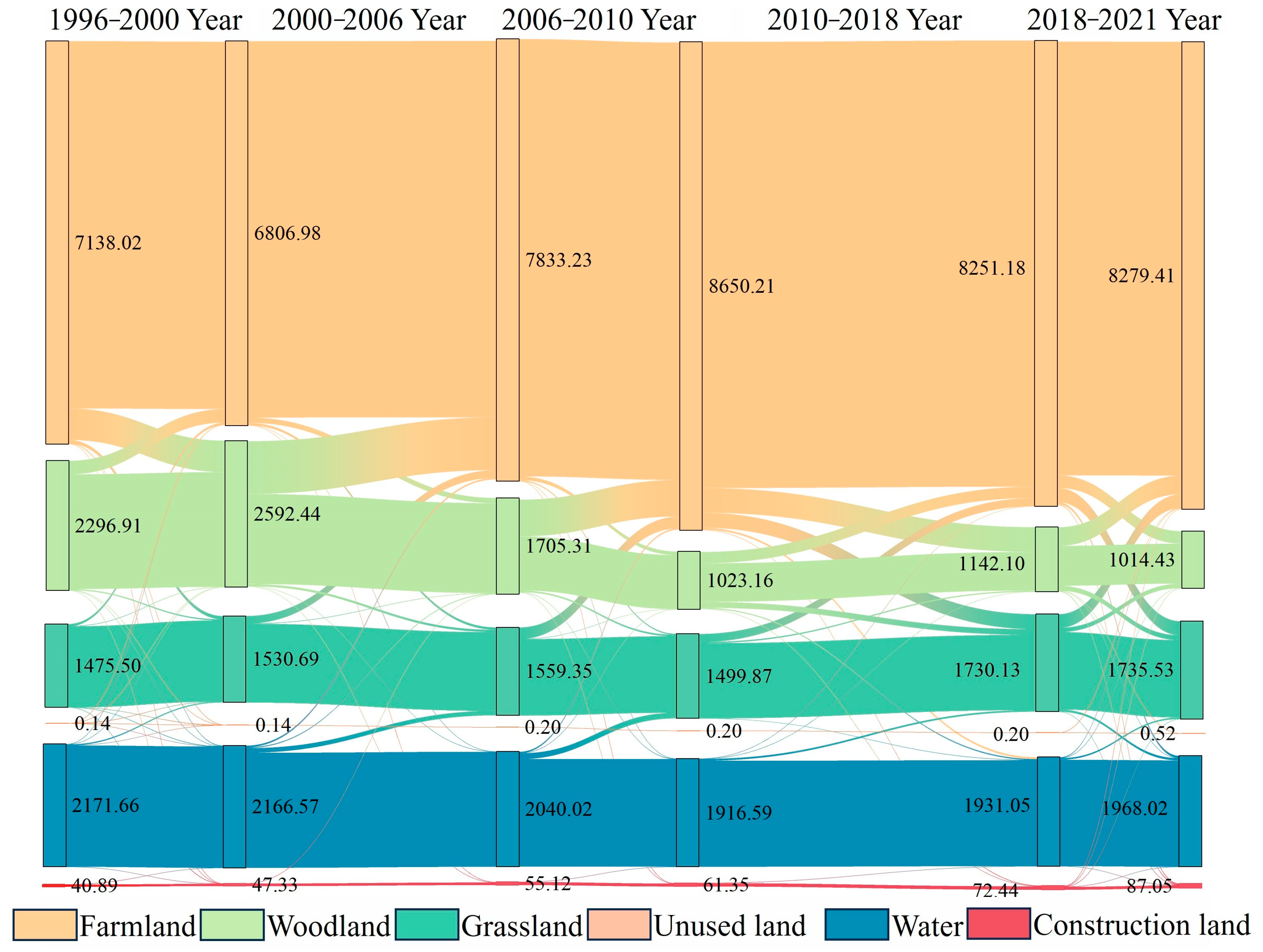
3.1. Spatial and Temporal Change Characteristics of Landscape Types

To comprehensively analyze the spatiotemporal change characteristics of wetland landscapes and understand the transformation patterns between different landscape types, this study constructed a time-series Sankey diagram to illustrate the flow dynamics among various landscape types (Figure 2). Between 1996 and 2021, the activities and transformations between landscape types within the region intensified year by year. The dominant landscape type was farmland, the area of which initially increased and then decreased. This trend is mainly because of the large-scale conversions from forest and grassland to farmland. The second most prominent landscape type was water bodies, which showed relatively stable changes during the study period but experienced a noticeable reduction between 2000 and 2010, primarily due to the conversion of water areas into grasslands. This shift resulted from the government’s protection plan for the Caohai Wetland, which was initiated in 2000. The grassland area exhibited an overall increasing trend despite significant internal losses; however, the inflow exceeded the outflow. Forest land experienced “M”-shaped patterns of changes. Between 1996 and 2000, the conversion from farmland to forest land was much greater than that from forest land to farmland, leading to the highest forest land area over the 25-year period. After 2000, there was a substantial reversal from forest land to farmland, causing a sharp decline in forestland areas, reaching its lowest point in 2010. The built-up land area steadily increased over the years, mainly at the expense of farmland, forestland, and grassland. Unused land remained unchanged from 1996 to 2018 but experienced shifts with farmland between 2018 and 2021; however, these changes did not significantly impact its total quantity.

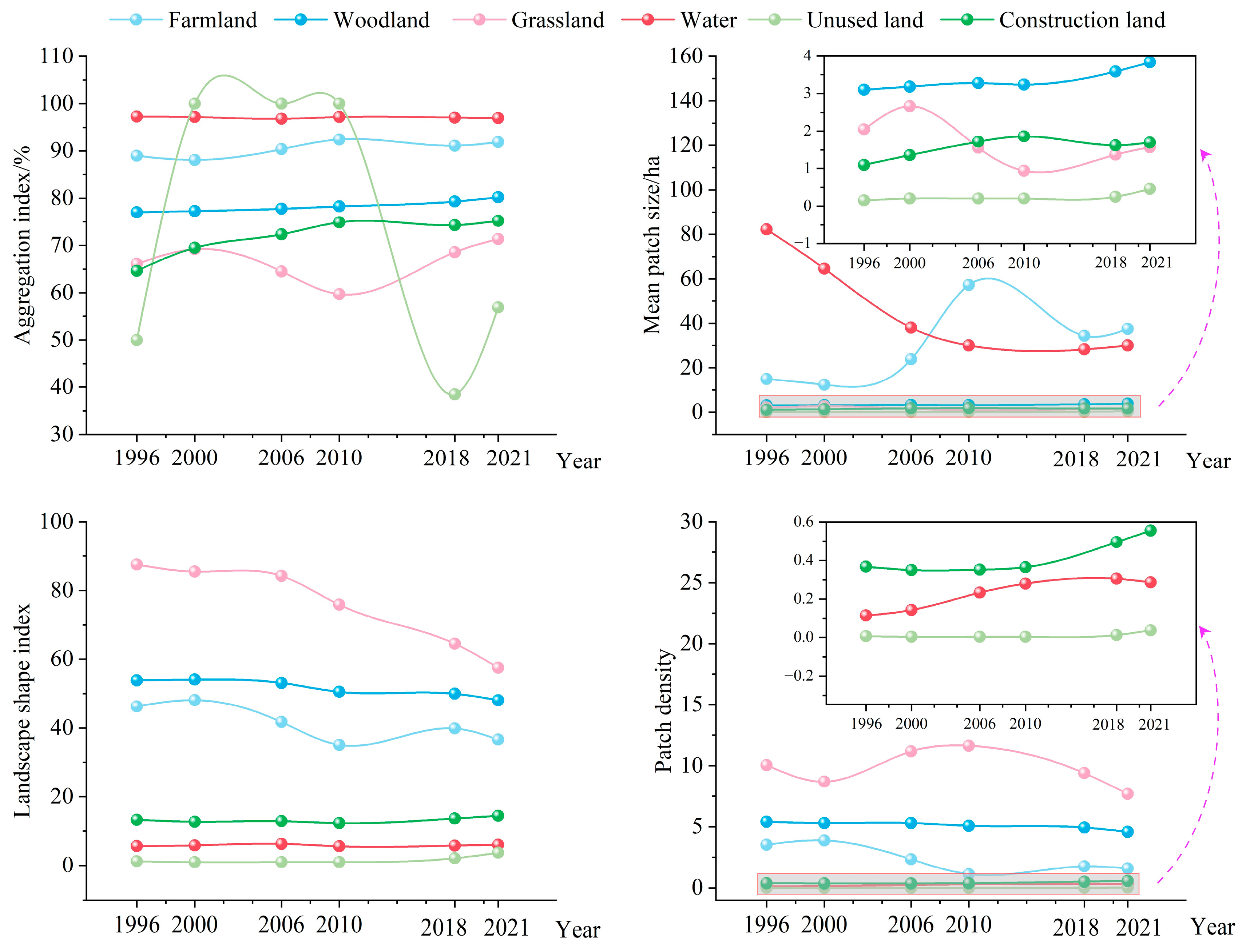
3.2. Spatial and Temporal Change Characteristics of Landscape Patterns at the Type Level

This study characterized the dominance of and changes in various landscape types using metrics such as the patch area (CA), percentage of landscape (PLAND), largest patch index (LPI), and number of patches (NPs). Based on patch area and PLAND, the predominant landscape types in the study area were farmland, forest, and grassland (Figure 3). Over time, farmland and grassland exhibited inverse trends in both patch area and PLAND, correlating with their mutual transitions observed in Figure 2. The other three landscape types exhibited relatively minor fluctuations. When considering LPI, the contrasting trends for farmland and grassland persisted, but there was a shift in dominance. Overall, the hierarchy was farmland > water bodies > grassland > forest > built-up land > unused land. Notably, between 2006 and 2010, the dominance of grassland was less pronounced than that of forests because of the substantial conversion of grassland into farmland. These transformations predominantly occurred in concentrated areas of contiguous grassland patches, leading to a reduction in LPI and the disruption of dominance. Conversely, the conversion of forest to farmland involved smaller forest patches, causing less disruption to contiguous areas. Regarding NP, farmland and grassland exhibited inverse trends, with the distribution ranking as grassland > forest > farmland > built-up land > water bodies > unused land. This indicates that grasslands and forests are more fragmented, whereas water bodies, unused land, and built-up areas tend to be more concentrated. In summary, farmland, grassland, water bodies, and forests play dominant roles in the study area, with intense interactions among them. Farmland plays a crucial role in maintaining the overall integrity of landscape patches, whereas grasslands, forests, and waterbodies provide auxiliary functions. Built-up and unused land exerts minimal influence on these dynamics.

To further explore the fragmentation of landscape types within the region, we used four key indices as follows: the aggregation index (AI), mean patch size (MPS), patch density (PD), and landscape shape index (LSI). These metrics provide a comprehensive characterization of fragmentation levels in wetland landscapes. AI reflects the extent to which patches of the same type cluster together, with higher values indicating greater aggregation and lower fragmentation. As shown in Figure 4, in 1996, grasslands exhibited less fragmentation than built-up areas. Overall, the fragmentation levels across all landscape types were ranked as follows: grassland > built-up land > forest > farmland > water bodies. Unused land displayed unique dynamics—it was the most fragmented in 1996 but exhibited the least amount of fragmentation between 2000 and 2010. By 2018 and 2021, it again became the most fragmented, indicating significant external influences during these periods. MPS serves as an indicator of fragmentation, with larger values indicating lower fragmentation. As shown in Figure 4, the fragmentation levels in 1996 and 2000 ranked as follows: unused land > built-up land > grassland > forest > farmland > water bodies. However, from 2006 onward, this order changed to the following: unused land > grassland > built-up land > forest > water bodies > farmland. The PD index, where higher values denote greater fragmentation, consistently ranked fragmentation levels as follows: grassland > forest > farmland > built-up land > water bodies > unused land.

Combining insights from AI, MPS, PD, NP, and the transitions among landscape types, it is evident that unused land and built-up areas occupy smaller proportions of the region and, thus, have a lesser impact on the overall landscape. Consequently, they were excluded from the specific fragmentation ranking. Overall, grasslands exhibited the highest degree of fragmentation, while water bodies exhibited the lowest. The LSI corroborates these findings by reflecting the complexity of patch shapes. Higher LSI values indicate more complex shapes and greater heterogeneity, leading to higher fragmentation. As shown in Figure 4, grasslands had the highest LSI values, followed by forests and farmlands, whereas built-up areas, water bodies, and unused land had relatively lower LSI values. This further underscores the fact that grasslands possess the most complex shapes and higher heterogeneity, resulting in greater fragmentation.

3.3. Spatial and Temporal Change Characteristics of Landscape Patterns at the Landscape Level

The above analysis examined the landscape characteristics of the region from the perspective of different landscape types. To further reflect the overall changes in the study area, we analyzed several indices: the landscape division index (DIVISION), AI, the Shannon evenness index (SHEI), Shannon diversity index (SHDI), PD, and contagion index (CONTAG). The results are summarized in

Table 8. Characteristics index of landscape patterns at the landscape level.

Year	DIVISION	CONTAG	AI	PD	SHDI	SHEI
1996	0.79	54.72	82.91	19.75	1.21	0.62
2000	0.84	54.31	82.57	18.52	1.33	0.64
2006	0.77	56.13	84.13	19.47	1.18	0.61
2010	0.63	60.62	86.78	18.59	1.07	0.55
2018	0.75	58.50	86.47	17.05	1.13	0.58
2021	0.73	59.49	87.41	14.89	1.21	0.58

. DIVISION reflects the extent to which landscapes within a region are divided into smaller patches and is often used to assess the impact of human activities on natural landscapes. Table 8 shows that between 1996 and 2021, DIVISION initially increased and then decreased, with values consistently above 0.63, indicating significant human interference and a relatively fragmented landscape. The highest value was recorded in 2000, while the lowest occurred in 2010, suggesting periods of significant human activity. Both CONTAG and AI indicate the degree of aggregation among landscape patches within a region. During the study period, CONTAG ranged from 54 to 60, suggesting that the landscape was neither completely uniform nor highly dispersed but in an intermediate state characterized by some mixing and clustering. From an ecological connectivity perspective, this indicates moderate connectivity within the landscape. The AI values ranged from 82 to 88 and showed an overall upward trend, indicating that similar landscape patches were clustered or aggregated. This contrasts somewhat with CONTAG, which may be more representative when considering the dominance of farmland and water bodies, as discussed in Section 3.1 and Figure 4. The PD values ranged from 14 to 20, indicating that the landscape was divided into many small patches but did not reach the level of extreme fragmentation. This represents a relatively complex landscape pattern with a rich spatial structure, which could pose certain ecological challenges. The SHDI values were approximately one, indicating low landscape diversity owing to farmland, water bodies, and forests occupying most of the area, with other patch types being either small, in proportion, or unevenly distributed. A lower diversity can make ecosystems more vulnerable to external disturbances, thereby reducing their buffering and recovery capacities. The SHEI values ranged from 0.55 to 0.65, indicating an uneven distribution of landscape types, reflecting a certain complexity and heterogeneity within the regional ecosystem. In summary, the study area exhibited significant landscape changes characterized by high fragmentation levels, the aggregation of specific landscape patches, moderate patch density, and low landscape diversity. These changes can reduce the buffering and recovery capacities of ecosystems, making them more susceptible to external disturbances.

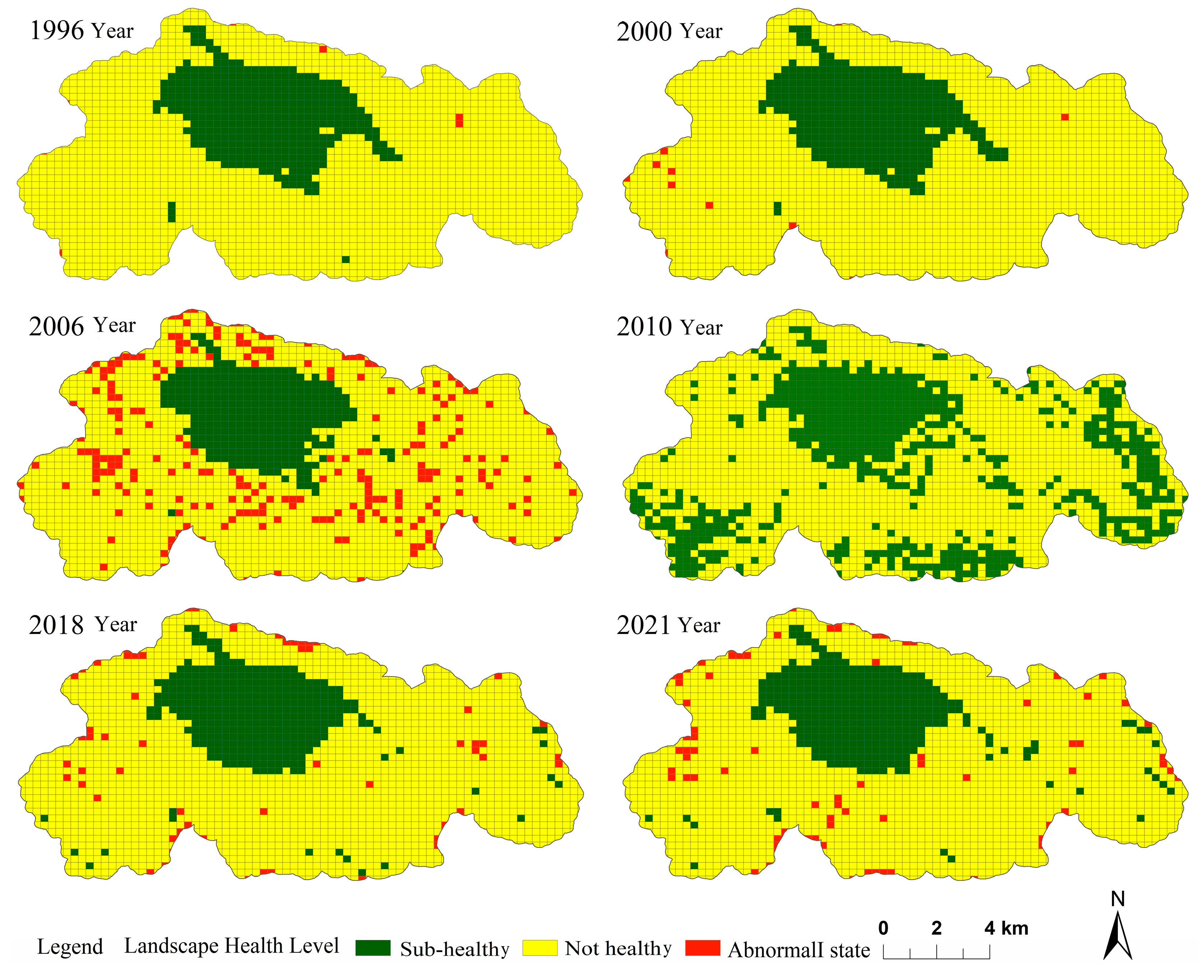
3.4. Comprehensive Evaluation of Wetland Ecosystem Health

This study conducted a statistical analysis of the mean ecological health diagnosis of each grid within the specific region to comprehensively evaluate the health status of the wetland ecosystem (

Table 9. Comprehensive evaluation results of wetland ecosystem health.

Year	Comprehensive Evaluation Value	Health Grade
1996	0.33	Not healthy
2000	0.32	Not healthy
2006	0.27	Not healthy
2010	0.35	Not healthy
2018	0.31	Not healthy
2021	0.31	Not healthy

). The results show that from 1996 to 2021, the overall health evaluation value of the wetland ecosystem consistently remained low, ranging between 0.27 and 0.35. All years were classified as “unhealthy”, indicating no significant improvement in the health status of the wetland ecosystem during this period, which remained in an unfavorable state. Specifically, the health evaluation value of the wetland ecosystem showed a declining trend from 1996 to 2006, decreasing from an initial value of 0.33 to its lowest point of 0.27. In 2010, the value of evaluation rose to its highest point of 0.35 but declined to 0.31 in 2018 and 2021 and remained stable thereafter. However, it remained within the unhealthy range. This reflects the severe challenges faced by the wetland ecosystem during this period. Although there were brief signs of improvement in 2010, they did not lead to a long-term, effective recovery. The persistently low health evaluation values underscore the ongoing difficulties and adverse conditions experienced by the wetland ecosystem over the years.

Further analysis of the health diagnosis values of different grid areas within the wetlands, as presented in

Table 10. Classification of landscape health diagnostic values for wetland grid areas.

Year	0–0.2 Abnormal State	0.2–0.4 Not Healthy	0.4–0.6 Sub-Healthy	0.6–0.8 Healthy	0.8–1 Very Healthy
1996	0.46%	82.37%	17.17%	0.00%	0.00%
2000	0.83%	82.27%	16.90%	0.00%	0.00%
2006	10.82%	74.49%	14.69%	0.00%	0.00%
2010	0.00%	69.48%	30.52%	0.00%	0.00%
2018	3.22%	80.99%	15.79%	0.00%	0.00%
2021	4.01%	79.74%	16.25%	0.00%	0.00%

and Figure 5, reveals that, except for 2010, “morbid” regions were present in all other years. Initially, these morbid areas were located on the periphery of the study area but gradually spread toward the center over time. In 2006, the proportion of “morbid” areas reached its peak at 10.82%, indicating particularly poor conditions during that year. The “unhealthy” category consistently accounted for the largest proportion across all years, underscoring the fact that most wetland grids have long been in an “unhealthy” state. The percentage of “unhealthy” areas was as high as 82.37% in 1996, decreased to its lowest point of 69.48% in 2010, and rebounded to 79.74% by 2021. Notably, 2010 witnessed the highest proportion of “sub-healthy” areas, reaching 30.52%, while this category remained at around 14–17% in other years. Throughout the study period, no grid area achieved a “healthy” or “very healthy” status, highlighting the severe health issues faced by the wetland ecosystem. This lack of recovery to an ideal state underscores the ongoing challenges and adverse conditions experienced by wetlands. These findings emphasize the critical need for targeted interventions and conservation efforts to address persistent health issues within wetland ecosystems.

In summary, the aforementioned results reveal that the wetland ecosystem generally remained in a poor state throughout the study period, with a consistently high proportion of areas falling into the “unhealthy” and “sub-healthy” categories. Although the data from 2010 showed an increase in “sub-healthy” areas, this did not establish a lasting trend. Consequently, the health status of the wetland ecosystem did not show significant improvement over the entire study period. The persistently low health evaluation values underscore the severe challenges faced by wetland ecosystems. The lack of any grid area achieving a “healthy” or “very healthy” status further emphasizes the extent of the ecological issues. This situation calls for more effective conservation measures to promote ecological recovery and sustainable development of wetland ecosystems. Targeted interventions are necessary to address ongoing health problems and mitigate adverse impacts on biodiversity and ecosystem services. Through concerted efforts, we hope to achieve meaningful improvements in the health and resilience of this vital ecosystem.

4. Discussion

The Grass Sea, a typical karst plateau wetland, has experienced significant changes in hydrology and its wetland areas [46]. Its fragile ecological environment has experienced severe degradation due to human activity, followed by deliberate efforts to restore and reshape the ecosystem. In 1972, large-scale anthropogenic drainage and cultivation nearly obliterated the Grass Sea, leading to severe regional ecological damage. The Guizhou Provincial Government initiated the recovery of the Grass Sea in 1980 and achieved preliminary restoration [26]. It was designated as a nature reserve in 1985 and was included in the list of national-level nature reserves in 1992, prompting increased protection efforts from various levels of government [25]. By 1996, the ecological health of the Grass Sea had improved, with fewer areas classified as morbid. However, between 1996 and 2006, the ecological health of the wetland gradually deteriorated with an increase in morbid areas that spread inward from the periphery, consistent with the findings of Han et al. [47]. This situation was particularly pronounced in 2006, mainly because of the rapid expansion of Weining County, population growth, and the significant discharge of domestic wastewater, garbage, and industrial and service waste, which severely polluted parts of the land and water bodies [48]. In 2010, ecological health showed noticeable improvement, with the disappearance of morbid areas. This was attributed to enhanced government protection measures, such as the approval of the “General Plan for the Guizhou Grass Sea National Nature Reserve” in 2005 and the establishment of the Caohai Wetland Management Committee in Bijie City in 2008. Years of comprehensive management gradually improved the ecological environment. However, from 2010 to 2021, morbid areas in the Grass Sea gradually increased again. This was, in part, because the comprehensive rectification and restoration work halted boat tourism, closed all docks, and prohibited fishing, swimming, pollution, and breeding within the lake, which allowed the Grass Sea to rest and recover. Owing to the relatively enclosed nature of the wetland lake, grass carp, carp, and other fish populations rapidly grew beyond the environmental carrying capacity, leading to water quality decline and impacting the surrounding ecological health. Qin et al. [49] indicated that the areas surrounding the Grass Sea wetland have high emissions of industrial and domestic wastewater and extensive use of fertilizers and pesticides, imposing significant pressure on the ecological health of the Grass Sea. The ecological health of the Grass Sea is largely influenced by human activities, necessitating greater emphasis on its protection and the adoption of more proactive and effective measures to enhance environmental quality, such as reducing pollution, restoring natural hydrological conditions, and protecting and reconstructing wetland vegetation. Moreover, considering the importance of wetlands in maintaining biodiversity, purifying water quality, and regulating floods, improving wetland health is not only essential for environmental protection but also represents a long-term investment in human society. Therefore, governments and relevant organizations should strengthen their support for wetland protection policies, formulate reasonable protective measures, and gradually improve the health status of wetland ecosystems to promote their self-recovery capabilities and sustainable development.

5. Conclusions

Considering both natural and social factors, a comprehensive ecological health evaluation index system was constructed for the karst plateau wetland landscape pattern based on 13 diagnostic indicators. The coefficient of variation method was used to calculate the weight of each indicator for different periods, and the wetland landscape’s ecological health evaluation index was applied to assess ecological health. The conclusions are as follows:

(1) Between 1996 and 2021, the conversion activities among landscape types increased annually. Farmland increased the most significantly, while forested areas decreased markedly. Built-up land and grasslands exhibited slight increases, whereas water bodies and unused land maintained a dynamic balance.

(2) Farmland and water bodies were the primary dominant landscapes in the region, followed by grasslands and forests. Built-up land and unused land exhibited the smallest dominance. Notably, grasslands were the most fragmented landscape type within the study area, exhibiting complex shape characteristics and high heterogeneity, whereas water bodies showed the lowest fragmentation, remaining relatively intact.

(3) From 1996 to 2021, the overall health evaluation value of the wetland ecosystem consistently remained at a low level (ranging from 0.27 to 0.35), with all years assessed as “unhealthy.”

(4) Throughout the study period, the “unhealthy” category accounted for the largest proportion each year. Except for 2010, some areas were diagnosed as “morbid” in all other years, with the proportion of morbid areas reaching its peak at 10.82% in 2006. Initially, these morbid areas were mainly distributed on the periphery of the study area but gradually spread towards the center over time.

References

1. Zhang, H.Y.; Long, E.; Cheng, W.M. Research on Dynamic Change and Effect Factors of Xianghai Wetland. J. Nat. Resour. 2005, 20, 613–620. [Google Scholar] [CrossRef]
2. Holland, M.M. Wetland Environment Gradients, Boundaries and Buffers; Mulamoottil, G., Warner, B.G., McBean, E.A., Eds.; CRC Press Inc.: Boca Raton, FL, USA, 1996; pp. 112–131. [Google Scholar]
3. Jiang, W.; Li, J.; Li, J.; Xie, Z.; Wang, W. Assessment of wetland ecosystem health in the Liaohe River Delta. Acta Ecol. Sin. 2005, 25, 408–415. [Google Scholar] [CrossRef]
4. Wang, Y.; Huang, H.; Peng, J.; Xie, S.; Yang, H.; Guo, F.; Tan, H. Occurrence and distribution of typical antibiotics in the aquatic environment of the wetland karst plateau in Guizhou. Environ. Chem. 2020, 39, 975–986. [Google Scholar] [CrossRef]
5. Xia, P.H.; Guan, Y.Z.; Yu, L.F. Carbon metabolic soil microbial community in Caohai Karst Plateau degraded wetland: A case study in southwest China. Acta Sci. Circumstantiae 2015, 35, 2549–2555. [Google Scholar] [CrossRef]
6. Liu, H.Y.; Li, Y.F.; Cao, X.; Hao, J.; Hu, J.; Zheng, N. The Current Problems and Perspectives of Landscape Research of Wetlands in China. Acta Geogr. Sin. 2009, 64, 1394–1401. [Google Scholar] [CrossRef]
7. Chen, Z.; Shang, H.; Yao, B. American wetland health assessment methods. Acta Ecol. Sin. 2009, 29, 5015–5022. [Google Scholar] [CrossRef]
8. Yang, H. Study on the Characteristics of Wetland Evolution and Ecosystem Health Evaluation in the Yellow River Delta. Master’s Thesis, North China University of Water Resources and Electric Power, Zhengzhou, China, 2019. [Google Scholar] [CrossRef]
9. Larson, J.S. Rapid assessment of wetlands: History and application to management in Mitsch. In Global Wetlands: Old World and New; Elsevier: Amsterdam, The Netherlands, 1994; pp. 623–636. [Google Scholar]
10. Zheng, Y. Research on the Evaluation of Wetland Ecosystem Health in Yanbian Prefecture. Master’s Thesis, Yanbian University, Yanji, China, 2018. [Google Scholar]
11. Yi, F.J.; Huang, D.; Liu, J.H.; Qiu, J.; Shi, Y.Y.; Li, R.D. The Change of Hanjiang River Basin Wetland and lts Ecological Health Assessment. J. Geo-Inf. Sci. 2017, 19, 70–79. [Google Scholar] [CrossRef]
12. Wang, H.N.; Yu, F.; Li, J. Health Assessment and Prediction of Wetland Ecosystem in Yangtze River Economic Belt. J. China Hydrol. 2023, 43, 78–83. [Google Scholar] [CrossRef]
13. Zhu, L.M.; Zhu, K.X.; Zeng, X.J. Evolution of landscape pattern and response of ecosystem service value in international wetland cities: A case study of Nanchang City. Ecol. Indic. 2023, 155, 110987. [Google Scholar] [CrossRef]
14. Yang, R.; Chen, Y.; Qiu, Y.; Lu, K.; Wang, X.; Sun, G.; Liang, Q.; Song, H.; Liu, S. Assessing the Landscape Ecological Health (LEH) of Wetlands: Research Content and Evaluation Methods (2000–2022). Water 2023, 15, 2410. [Google Scholar] [CrossRef]
15. Yadav, P.K.; Jha, P.; Joy, M.S.; Bansal, T. Ecosystem health assessment of East Kolkata Wetlands, India: Implications for environmental sustainability. J. Environ. Manag. 2024, 366, 121809. [Google Scholar] [CrossRef] [PubMed]
16. Zhu, M.; Dong, B.; Cui, Y.; Zhang, S.; Ni, Y.; Yang, F.; Xu, W. Shengjin Lake wetland ecosystem health assessment and the response of overwintering migratory birds. J. Anhui Agric. Univ. 2020, 47, 88–94. [Google Scholar] [CrossRef]
17. Li, R.R. Analysis of Water Environment Evolution and Ecological Risk Assessment of Chagan Lake Wetland. Ph.D. Thesis, Graduate School of the Chinese Academy of Sciences (Northeast Institute of Geography and Agroecology), Changchun, China, 2014. [Google Scholar]
18. Rapport, D.J. Evolution of Indicators of Ecosystem Health. In Ecological Indicators; Springer US: Boston, MA, USA, 1992. [Google Scholar] [CrossRef]
19. Brooks, R.P.; Brinson, M.M.; Havens, K.J.; Hershner, C.S.; Rheinhardt, R.D.; Wardrop, D.H.; Whigham, D.F.; Jacobs, A.D.; Rubbo, J.M. Proposed Hydrogeomorphic Classification for Wetlands of the Mid-Atlantic Region, USA. Wetlands 2011, 31, 207–219. [Google Scholar] [CrossRef]
20. Gebo, N.A.; Brooks, R.P. Hydrogeomorphic (HGM) Assessments of Mitigation Sites Compared to Natural Reference Wetlands in Pennsylvania. Wetlands 2012, 32, 321–331. [Google Scholar] [CrossRef]
21. Liu, L.; Zhang, Y.; Li, P.; Feng, J.; Ye, T.; Luo, H.; Hu, Y.; Pan, L.; Hu, F.; Tan, W.; et al. Ecosystem Health Assessment of Typical Lake Wetlands in Wuhan City: A Case Study of Tang xun Lake. Resour. Environ. Eng. 2022, 36, 773–781. [Google Scholar] [CrossRef]
22. He, Z.; Zheng, Z.J. Health Assessment of Coastal Wetland Ecosystems in Guangxi and Guangdong. Sci. Technol. Eng. 2023, 23, 14896–14904. [Google Scholar] [CrossRef]
23. Wang, W.; Chen, W.F.; Li, Q.G.; Wang, X.; Ma, H. Assessment indicator system for ecosystem health of wetlands in Yellow River Delta. Water Resour. Prot. 2012, 28, 13–16. [Google Scholar] [CrossRef]
24. He, Y.; Yang, H.; Wang, J.; Yu, W.; Yin, C.; Xu, D.; Tang, X.; Wu, J. Improvement of Water Quality by Ecological Restoration in Heavily Polluted Area of Caohai Lake, Guizhou Province. J. Hydroecol. 2021, 42, 78–85. [Google Scholar] [CrossRef]
25. Ren, J.; Yang, K.; Wang, Z.; Mo, S.; Chen, Q.; Feng, T. Study on spatial-temporal change of land use pattern in Caohai Lake wetland area. Yangtze River 2018, 49, 18–23. [Google Scholar] [CrossRef]
26. Ren, X.D.; Huang, M.J. Research on Integrated Management of Caohai Watershed. Ecol. Econ. 2008, 5, 147–151. [Google Scholar]
27. Pan, S.B.; Ren, X.D. An analysis on quantitative classification and ordination of aquatic plant communities in Caohai natural reserve. J. Biol. 2010, 27, 60–63+76. [Google Scholar] [CrossRef]
28. Yang, J.; Huang, X. The 30 m annual land cover dataset and its dynamics in China from 1990 to 2019. Earth Syst. Sci. Data 2021, 13, 3907–3925. [Google Scholar] [CrossRef]
29. Yang, F.; Yang, L.Y.; Fang, Q.Y.; Yang, X. Impact of landscape pattern on habitat quality in the Yangtze River Economic Belt from 2000 to 2030. Ecol. Indic. 2024, 166, 112480. [Google Scholar] [CrossRef]
30. Hu, J.Y.; Zhang, J.X.; Li, Y.Q. Exploring the spatial and temporal driving mechanisms of landscape patterns on habitat quality in a city undergoing rapid urbanization based on GTWR and MGWR: The case of Nanjing, China. Ecol. Indic. 2022, 143, 109333. [Google Scholar] [CrossRef]
31. Wu, J.G.; Wei, G.; Paul, T. Tueller. Effects of Changing Spatial Scale on the Results of Statistical Analysis with Landscape Data: A Case Study. Geogr. Inf. Sci. 1997, 3, 30–41. [Google Scholar] [CrossRef]
32. Xu, Y.; Yang, F.; Yan, C.Z. Ecological health assessment of urban wetland in Xiong’an based on landscape pattern. Acta Ecol. Sin. 2020, 40, 7132–7142. [Google Scholar] [CrossRef]
33. Jin, M.L. Comprehensive assessment of urban lake wetlands in the Jiangnan water network: Implementation of ecosystem health models. J. Nat. Conserv. 2025, 84, 126820. [Google Scholar] [CrossRef]
34. Zhang, Y.; Zang, P.; Guo, H.; Yang, G. Wetlands ecological security assessment in lower reaches of Taoerhe river connected with Nenjiang river using modified PSR model. HydroResearch 2023, 6, 16–165. [Google Scholar] [CrossRef]
35. Fentaw, G.; Mezgebu, A.; Wondie, A.; Getnet, B. Ecological health assessment of Ethiopian wetlands: Review and synthesis. Environ. Sustain. Indic. 2022, 15, 100194. [Google Scholar] [CrossRef]
36. Hou, M.; Li, L.; Yu, H.; Jin, R.; Zhu, W. Ecological security evaluation of wetlands in Changbai Mountain area based on DPSIRM model. Ecol. Indic. 2024, 160, 111773. [Google Scholar] [CrossRef]
37. Han, X.; Hu, J.; Liu, C.; Wang, X. Mountain landscape health diagnosis and pattern evolution based on remote sensing: Case study in Xinjiang Tianshan Karajun-Kurdening. Acta Ecol. Sin. 2021, 41, 6451–6465. [Google Scholar] [CrossRef]
38. Yin, L.J.; Zhou, Z.F.; Zhu, C.L.; Shang, M.J. Geomorphological Differentiation Characteristics of Land Use Change in Karst Rocky Desertification Area-A Case of Guanling-Zhenfeng Huajiang Rocky Desertification Comprehensive Demonstration Zone in Guizhou Province. Bull. Soil Water Conserv. 2020, 40, 37–46. [Google Scholar] [CrossRef]
39. Zhou, Q.; Peng, C.; Liu, X.; Xiang, Y.; Zhou, L. Ecosystem Health Assessment of Water Level Fluctuating Zone in ThreeGorges Reservoir Area Based on VOR Model. Res. Soil Water Conserv. 2022, 29, 310–318. [Google Scholar] [CrossRef]
40. Jia, K.; Yao, Y.; Wei, X.; Gao, S.; Jiang, B.; Zhao, X. A Review on Fractional Vegetation Cover Estimation Using Remote Sensing. Adv. Earth Sci. 2013, 28, 774–782. [Google Scholar] [CrossRef]
41. Liu, M.H.; Dong, G.H. Ecosystem health assessment and driving force analysis in Qinhuangdao area based on RS & GlS. Geogr. Res. 2006, 25, 930–938. [Google Scholar] [CrossRef]
42. Xie, G.D.; Lu, C.X.; Xiao, Y.; Zheng, D. The Economic Evaluation of Grassland Ecosystem Services in Qinghai-Tibet Plateau. Mt. Res. 2003, 21, 50–55. [Google Scholar] [CrossRef]
43. Wang, D.; Lan, A.; Fan, Z.; Zou, Y.; Li, W.; Wang, R. Scenario Modeling of Response of Land Use Change to Ecosystem Service Values in A Typical Karst Region. Res. Soil Water Conserv. 2024, 31, 308–315+325. [Google Scholar] [CrossRef]
44. Li, Y.; Feng, X.; Wu, L.H. Dynamic Simulation of Land Use and Response of Ecosystem Service Value in PUDING County from 1973 to 2030 Carsologica Sinica. pp. 1–19. Available online: http://kns.cnki.net/kcms/detail/45.1157.P.20240827.1644.002.html (accessed on 20 December 2024).
45. Zhang, M. Ecosystem Health Evaluation Based On Landscape Pattern. Master’s Thesis, Hunan Normal University, Changsha, China, 2014. [Google Scholar]
46. Biological Research Institute of Guizhou Provincial Academy of Sciences. Scientific Investigation Report of Caohai; Guizhou People’s Publishing House: Guiyang, China, 1986. [Google Scholar]
47. Han, H.Q.; Su, Z.H.; Luo, X.Q.; Cai, G. Habitat Quality Change in Caohai Nature Reserve from 2000 to 2010. J. Southwest For. Univ. 2016, 36, 158–163. [Google Scholar] [CrossRef]
48. Qin, Q.; Chen, Z.Q.; Yao, S.M. Ecological Safety Evaluation of Caohai Lake Wetland in Weining. J. Hydroecol. 2018, 39, 27–33. [Google Scholar] [CrossRef]
49. Qin, Q.; Liang, Z.M.; Liu, A.L.; Zhao, Z.Y. The ecological safety evaluation of plateau wetland based on DPSIRM framework mode. J. Glaciol. Geocryol. 2020, 42, 1363–1375. [Google Scholar] [CrossRef]
Figure 1. Schematic diagram of the study area.
Water 17 00537 g001
Figure 2. Temporal Sankey diagram of landscape-type transitions.
Water 17 00537 g002
Figure 3. Dominance indices of landscape patterns at the type level.
Water 17 00537 g003
Figure 4. Fragmentation index of landscape patterns at the type level.
Water 17 00537 g004
Figure 5. Distribution of landscape health diagnosis in various grid areas of wetlands.
Water 17 00537 g005