Article

Prediction of Reservoir-Type Landslide Displacement Based on the Displacement Vector Angle and a Long Short-Term Memory Neural Network

1
Key Laboratory of Geological Safety of Coastal Urban Underground Space, Ministry of Natural Resources, Qingdao 266101, China
2
Department of Civil Engineering, Qingdao University of Technology, Qingdao 266033, China
*
Author to whom correspondence should be addressed.
Water 2025, 17(4), 499; https://doi.org/10.3390/w17040499
Submission received: 6 January 2025 / Revised: 9 February 2025 / Accepted: 9 February 2025 / Published: 11 February 2025

Abstract

:
Reservoir-type accumulation layer landslides have strong destructive force and complex displacement generation mechanisms. In this paper, the slope stability evaluation parameter of the displacement vector angle is introduced, and a rolling landslide displacement prediction method is proposed based on long short-term memory (LSTM) neural network. First, grey correlation analysis was employed to quantify the correlations between reservoir water level, rainfall patterns, cumulative displacement, and displacement vector angles with landslide displacement, thereby assessing the viability of incorporating displacement vector angles as predictive input features. Second, building upon the original study, historical displacement, displacement vector angle, and their combination are added as input features to assess the impact of various feature combinations on landslide displacement prediction outcomes. Thirdly, the LSTM model with different sliding window sizes is constructed to control different amounts of historical input data under different feature combinations. Finally, the impact of various feature combinations and varying amounts of historical inputs on landslide displacement prediction is assessed to identify the most effective prediction method. The method’s reliability is validated using actual monitoring data from the Bazimen landslide in the Three Gorges Reservoir area. The prediction results align with the monitoring data, confirming the feasibility of using the displacement vector angle as an input feature in the neural network for landslide displacement prediction.

1. Introduction

A reservoir-type accumulation layer landslide [1,2,3] refers to a special type of landslide in which the accumulation layer located on the reservoir bank or in the reservoir area slides under the action of reservoir water storage, which is the result of the coupled action of a variety of factors [4,5,6], including the following: reservoir water storage increases the water table in the reservoir area, resulting in an increase in the internal pore water pressure of the accumulation layer, and a decrease in the effective stress, which weakens the shear strength of the accumulation layer, and is prone to sliding [7]; when the reservoir water is impounded, the water level rises, the slope angle of the bank is subject to scouring and erosion, resulting in the expansion of the slope angle, which increases the probability of landslides [8]; after the reservoir impoundment, the soil under the accumulation layer is subject to water pressure, and the change of the self-weight stress leads to the change in stability [9]; the external forces such as earthquakes, rainfall and other external forces may lead to the occurrence of the issues in the accumulation layer, exacerbating the occurrence of landslides, etc. [10]. Due to the complex and diverse formation conditions of reservoir-type stacked-layer landslides, accurate and effective landslide displacement prediction methods have been under constant exploration, and there is an urgent need for accurate, effective early warning and forecasting methods for this type of landslide hazard [11].
Currently, there are four main types of landslide prediction models:
Physico-mechanical model [12,13]. This model is based on the mechanical properties and geological structure of the landslide body, and predicts the displacement of the landslide by analyzing the force on the landslide body and the deformation characteristics of the rock-soil layer, etc. Miao et al. [14] developed a Verhulst-Grey model for landslide time prediction based on the improved Saito method, and verified its reliability by using the landslide monitoring data. To realize rainfall-type landslide prediction for landslides in the Hulu Kelang area, Kim et al. [15] proposed the YS-Slope model by considering the groundwater level and rainfall infiltration on soil stability. Jeong et al. [16] assessed the stability of shallow landslides in the Hulu Kelang area by combining the GIS physical model, YS-Slope, with a geohydrological model. Physico-mechanical models have numerous parameters and usually require a large number of geologic parameters and site data such as groundwater level, soil properties, rainfall characteristics, topography, and anthropogenic activities for accurate prediction [17].
Statistical modelling [18]. Statistical models build mathematical models to predict landslide displacements by statistically analyzing historical landslide events and related factors. Yang et al. [19] regarded the landslide displacement prediction problem as a time series regression problem with a limited number of training samples, and proposed a probabilistic landslide displacement prediction model with quantified cognitive uncertainty, whose prediction accuracy is better than other probabilistic prediction models. Ma et al. [20] combined the Newmark model and two statistical analysis models (logistic regression and support vector machine, LR and SVM) with critical acceleration ac data to assess earthquake landslide hazard. Statistical models often employ probabilistic statistics, regression analysis, and cluster analysis, which usually require a large amount of historical data for modelling and analysis, and the incompleteness of the data in some specific cases limits their applicability and also affects the accuracy of the model [21].
Numerical simulation [22]. The development trend and displacement of landslides were predicted by numerical calculations. Jiang et al. [22] took the bridgehead landslide on the side of the Three Gorges reservoir area as an example, and through numerical simulation and experimental testing, it was found that the initial stage of the landslide deformation was mainly affected by seepage, and the later stage was mainly affected by consolidation. Dai et al. [23] proposed a landslide early warning method based on dynamic bandwidth allocation (DBA)-long short-term memory (LSTM) algorithm by combining machine learning and numerical simulation methods. Zhao et al. [24] conducted finite element numerical simulation of the Shuping landslide process, revealing the important role of rainfall in the occurrence of Shuping landslides. Xu et al. [25] proposed to use the numerical simulation results to expand the dataset required for deep learning, and constructed a slope displacement prediction model combining numerical simulation and deep learning to improve the prediction accuracy. Numerical simulation is now widely used in landslide displacement prediction, but its dependence on model parameter selection significantly limits the accuracy of prediction results.
Machine learning model [26,27]. Machine learning algorithms are used to learn and train the landslide prediction data, and construct a model to predict landslide displacement. Miao et al. [28] established an additive time series model for landslide displacement prediction by analyzing the deformation characteristics of the Baishui River landslide, and predicted the displacement change of the landslide. Zhang et al. [29] proposed a landslide dynamic displacement prediction method based on the combination of gated recurrent unit (GRU) and time series analysis method: the accuracy of prediction was better than that of support vector machine (SVM). Zhou et al. [30] examined the rainfall, reservoir level, and landslide stepwise deformation characteristics, and proposed a landslide prediction method based on the PSO-SVM coupled model. They concluded that the rainfall and the reservoir level were the dominant factors affecting most landslides in Three Gorges Reservoir area. Huang et al. [31] proposed a multivariate chaotic extreme learning machine (ELM) model to predict the landslide displacements of reservoirs in the Three Gorges reservoir area. The model prediction accuracy is better than that of the univariate chaotic ELM model and the multivariate chaotic PSO-SVM model. Machine learning models, leveraging their robust data processing capabilities, automated modeling proficiency, and adaptability to complex nonlinear relationships, can circumvent the simplified assumptions inherent in traditional physical mechanics models, statistical models, and numerical simulation models [32]. By reducing reliance on physical theories and assumptions, these models can fully exploit data for predictive purposes, thereby addressing some of the limitations of conventional methods in terms of accuracy, efficiency, and applicability. However, no study has yet used the displacement vector angle, a landslide stability evaluation parameter, for landslide displacement prediction, which limits the comprehensiveness and innovation of the model.
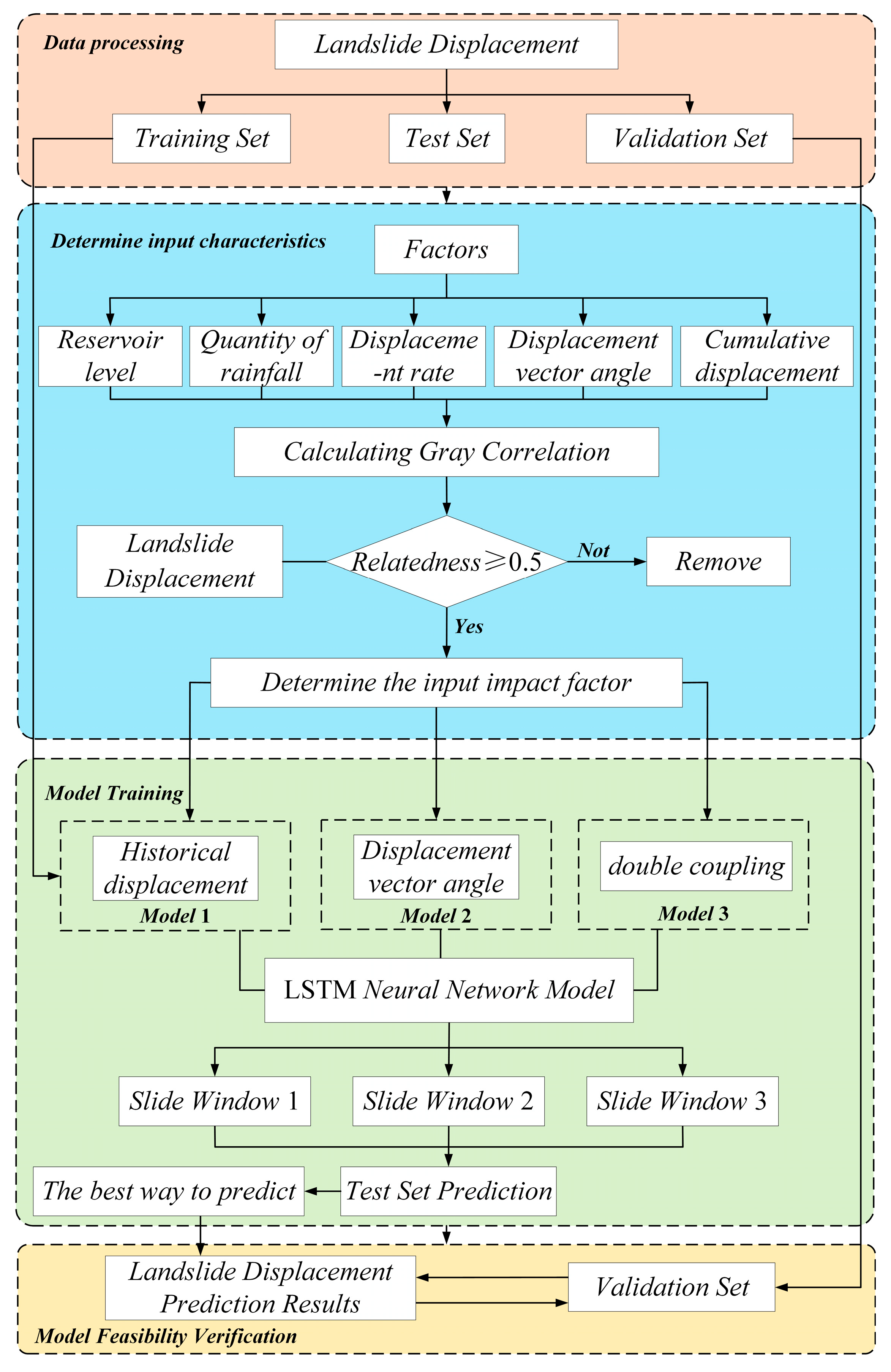
To investigate the potential of using displacement vector angles as input features for predicting landslide displacement, this study introduces historical displacement and displacement vector angles, along with reservoir water levels, rainfall, and displacement rates, as inputs to neural networks. Different feature combinations are constructed to predict landslide displacement. Gray relational analysis is employed to determine the correlation between displacement vector angles, reservoir water levels, rainfall, displacement rates, and landslide displacement, providing a preliminary assessment of the feasibility of using displacement vector angles as input features. By establishing LSTM neural network models with varying sliding window sizes, the impact of different feature combinations and sliding window sizes on landslide displacement prediction is evaluated and analyzed, thereby assessing the potential of displacement vector angles as input features for predicting landslide displacement.

2. Theory of Displacement Analysis and Prediction of Landslides in Stacked Layers

2.1. Displacement Vector Angle

The displacement vector angle is defined as the angle corresponding to the arctangent of the ratio of the vertical displacement to the horizontal displacement of a node [33]. The displacement vector angle can characterize the direction of the displacement field, which is affected by the horizontal and vertical displacements together. The vector angles formed by displacements of different natures are also characterized by different features.
Through the monitoring data, the horizontal displacement S(x) and vertical displacement S(y) of each monitoring point in the time interval t are calculated to obtain the slope displacement vector angle, as follows:
θ = arctan S ( y ) S ( x )
where θ is the displacement vector angle, S(y) denotes the vertical displacement, and S(x) is the horizontal displacement. The sign of the displacement vector angle only indicates the direction, not magnitude.

2.2. LSTM Neural Network Model

LSTM [34] is a special type of Recurrent Neural Network (RNN). Compared with the traditional RNN structure, LSTM is able to capture long-term dependencies in time series data through the gating mechanism and the operation of the memory unit, which improves the performance and generalization ability of the model. The LSTM network structure contains input gates, forgetting gates, internal states, and output gates (Figure 1).
The computational flow of the LSTM is described below.
The role of the forgetting gate is to help the model deal with long-term dependence and memorize long sequence information by controlling the flow of information to improve the time series prediction effect, which is calculated as follows:
f t = σ ( W f [ h t 1 , x t ] + b f )
where ft is the output of the forgetting gate; Wf and bf represent the weight matrix and bias vector of the forgetting gate; ht−1 denotes the hidden state of the previous time step; xt is the input of the current time step; and σ is the sigmoid function.
The output gate controls whether the current input information is stored in the memory cell or not, and is calculated as follows:
i t = σ ( W i [ h t 1 , x t ] + b i )
where it refers to the inputs; Wi and bi are the weight matrices and bias vectors of the input gates.
According to the current input and the hidden state of the previous moment as well as the forgetting gate and the outputs of the inputs, the content of the memory cell is updated, and the updating process is calculated thus:
C ~ t = tanh ( W C [ h t 1 , x t ] + b C )
where C ~ t is a new candidate memory cell; Wc and bc represent the weight matrix and bias vector used to update the memory cell.
The outputs control the output of the current time step, and their outputs are calculated thus:
o t = σ ( W o [ h t 1 , x t ] + b o )
The hidden states and outputs of the current time step are updated based on the current inputs and contents of the memory cell and the outputs of the input gate, forget gate and output gate, and the update process is as follows:
C t = f t C t 1 + i t C ˜ t
h t = o t tanh ( C t )
where Ct is the content of the memory cell for the current time step and ht denotes the current time step hidden state.

2.3. Sliding Window

Sliding windows [35] are a widely used technique for processing sequence data. This method involves extracting a subset of data by defining a fixed-length window on the input sequence and incrementally shifting it along the time axis or sequence dimension. At each step, the data within the window (historical information) is fed as input to the model, while data outside the window are ignored. By varying the window size, one can control the model’s retention of historical data and its contextual dependence.
The size of the sliding window governs the amount of historical information incorporated into the model, thereby adjusting the extent of contextual dependence in data processing. Specifically, the window size determines the span of input data the model receives at a given time, i.e., the history length. This technique helps balance the detailed capture of local information with the learning of global patterns when modeling time-series data. By adjusting the window size, the model’s capacity to remember past inputs and their influence can be controlled, thus optimizing both prediction performance and computational efficiency. The core calculation is as follows:
x i = x i w + 1 ,   x i w + 2 ,   ,   x { i }
where xi is the data sequence of the ith window; w is the window size; and xi−j refer to the i−jth time step data.

3. Landslide Displacement Prediction Method Based on the Displacement Vector Angle and LSTM Neural Network

The landslide displacement monitoring data as a displacement time series can be used as a neural network input to predict the future data by rolling the influencing factors such as reservoir level, rainfall, displacement rate and cumulative displacement. The idea is to obtain monitoring data pertaining to reservoir water level, rainfall and landslide displacement, then use grey correlation to assess the degree of correlation between each influencing factor and displacement, so as to determine the number of input features. Consequently, with different combinations of input features, different sizes of sliding windows are set up, and the best prediction method is selected by comparative analysis. The specific process is shown in Figure 2.
The specific implementation of landslide displacement prediction for stacked layers based on the displacement vector angle and LSTM neural network is described below.
(1)
Measured data acquisition and preprocessing of landslide displacement: the measured data pertaining to landslide reservoir water level, rainfall, displacement, etc. are acquired and divided into training, validation and test sets. The training and validation sets are used to train the model and adjust the model parameters, and the test set is used to verify the reliability of the model;
(2)
Determination of the number of input features. Grey correlation analysis is used to estimate the grey correlation between each influencing factor and displacement, calculate the grey correlation coefficient, and select those results greater than, or equal to, 0.5 as the network input;
(3)
Setting feature combinations: on the basis of the traditional input features (reservoir level, rainfall, displacement rate and cumulative displacement), the historical displacement is added as feature combination 1, the displacement vector angle is added as feature combination 2, and the two are coupled together as feature combination 3 to analyze the effects of different feature combinations on the prediction results;
(4)
Setting of the sliding window: different sizes of sliding windows are set, i.e., predict one displacement for each measurement, predict one displacement for every two measurements, predict one displacement for every three measurements, to estimate the effects of different sizes of sliding windows on the prediction results and select the best method.
(5)
Verification of the reliability of the model: the aforementioned best prediction method is used to predict the future data, and compare with the measured landslide displacement data to verify the reliability of the model.

4. Engineering Applications

4.1. Engineering Case Study

4.1.1. Project Overview

The Bazimen landslide is located in the near-dam section of the Three Gorges reservoir area (Figure 3). The landslide is high in the west and low in the east, in the shape of a ladder, with an elevation of 55~280 m. The total length of the landslide is 520 m. The slope is low in the front and high in the back, with the front edge of 20°~25° and the middle and back part of the slope 35°~40°. The upper part of the slope is 100~110 m wide and the lower part is 350 m wide. The upper part of the slope is 100~110 m wide, and the lower part is 350 m wide, and the whole slope is spreading to the river in the shape of a skip, and the front edge of the slope is flooded by the water storage from 55~156 m. The main sliding direction of the landslide is NW112°, the front edge is Xiangxi River, and the shear exit elevation is 65 m. The total area is about 117,800 m2, and the total volume is c. 2 × 10⁶ m3.
There are 10 deformation monitoring points at the Bazimen landslide, namely ZG110, ZG111, GSC1~GSC4, GSC5, GSC7~GSC9 (Figure 3). The ZG series of monitoring points are the earliest to be used, with 110 and 111 located in the front and center of the landslide, respectively, and the GSC series of monitoring points have a wide distribution, covering the rear to the front, and the north to the south side of the landslide.

4.1.2. Pre-Processing of Landslide Monitoring Data

Four GPS deformation monitoring points (ZG109, ZG110, ZG111, and ZG112) were deployed within the landslide area, forming two longitudinal (nearly east-west) monitoring profiles. A U.S. Ten Pao GPS receiver, with a planimetry accuracy of 5 + 1 ppm, was used for surface displacement and deformation monitoring of the landslides. At the same time, two GPS datum points (ZG06 and ZGJ6) were deployed on the stabilized hills on the outskirts of the landslide area to accurately measure the surface displacement of the landslide body.
Taking the measured data of monitoring point ZG110 as the research object, the monitoring time was from January 2006 to December 2012, and the data were collected once a month, giving a total of 84 measurements; the landslide displacement is shown in Figure 4. The monthly average reservoir level was used for the reservoir level, and the monthly cumulative rainfall was used for the rainfall, and the monthly displacement rate, displacement vector angle, and cumulative displacement were calculated. The landslide displacement was collected once a month. Considering that the symbols of the vectors such as displacement rate, displacement vector angle and landslide displacement only indicate the direction, not the specific size. The data herein are taken as absolute values for carryover calculation.
The first 70% of the landslide monitoring data was used as the training set to train the model, the second 15% of the monitoring data was used as the validation set, and to verify the applicability of the model, the remaining 15% of the data was extracted from 2016–2017 as the test set. The computational process of this paper’s method is implemented through MATLAB™ programming. Considering the different prediction results of landslide displacement under different feature combinations, different landslide displacement prediction models were established according to different feature combinations, named as Model I, Model II and Model III, to analyze the effects of different feature combinations on the prediction results. To determine the influence of the sliding window size on the prediction results, three different sizes of sliding window training models are constructed: predict one displacement for each measurement, predict one displacement for every two measurements, predict one displacement for every three measurements. (Table 1).

4.2. Analysis of the Rationality of the Selection of Influencing Factors

Studies have shown that reservoir water level and rainfall are two important influencing factors that induce the displacement of reservoir-type stacked layer landslides. When landslides undergo changes in displacement, their displacement rates, cumulative displacements, and displacement vector angles change significantly. These variables can more accurately characterize the trends at different stages of slope stabilization.
To evaluate the potential of using displacement vector angles as an input feature for predicting landslide displacements, gray correlation analysis was employed to quantify the correlation between displacement vector angles and landslide displacements. This analysis provided a preliminary assessment of the feasibility of utilizing displacement vector angles as input features for landslide displacement prediction. Grey correlation analysis is a data-analysis method that can reveal the degree of association between variables. In the grey correlation model, when the resolution coefficient ρ is 0.5 (or greater), the closer the correlation is to 1, the higher the degree of correlation between the two variables and the closer the relationship between them. The above influencing factor components and displacement components are subjected to grey correlation analysis, and the calculation results are listed in Table 2. The degree of correlation between each influencing factor component and displacement component is as follows: cumulative displacement > rainfall > displacement vector angle > reservoir level > displacement rate, and the correlation between each influencing factor and displacement component is close to 1. It is thus concluded that the chosen influencing factors have a strong correlation with the displacement component.

4.3. Sliding Window Selection

In order to determine the influence of the LSTM model with different sliding windows on prediction accuracy, LSTM models with incremental sliding window sizes were used to predict the landslide displacements. The evaluation index values for landslide displacement prediction with different sliding windows are shown in Table 3. The calculation results show that when the sliding window size is set between 1 and 3, the root mean square error (RMSE), mean absolute error (MAE), and the mean absolute percentage error (MAPE) of the model are small, and the correlation coefficient R2 can reach about 0.9, indicating a certain level of prediction accuracy. However, with the increase in sliding window size, the prediction accuracy shows a decreasing trend. For this reason, the sliding window size selected in this paper is 1–3.

4.4. Landslide Displacement Prediction

After several debugging sessions, the parameters of the LSTM model are determined as follows: the total number of training rounds is 250, the number of hidden units is 128, the initial learning rate is 0.05, and the L2 regularization parameter is 0.0001. To determine the optimal prediction method, the evaluation metrics such as the root mean square error (RMSE), mean absolute error (MAE), mean absolute percentage error (MAPE), and correlation coefficient R2 are used to determine the accuracy of prediction.

4.4.1. Influence of Historical Displacements on Landslide Displacement Prediction Results (Model I)

Historical displacement is closely related to displacement vector angles, and for this reason, the effect of historical displacements on landslide displacement prediction results is first explored. Reservoir level, rainfall, displacement rate, cumulative displacement, and historical displacement are used as network inputs, and landslide displacements are used as network outputs, with a network structure of 5-1 (Model I). The displacement prediction results are illustrated in Figure 5. Table 4 shows the evaluation index values of landslide displacement prediction for the three sliding windows corresponding to Model I. The computational results in Figure 5 and Table 3 show that the root mean squared error (RMSE), mean absolute error (MAE), and mean absolute percentage error (MAPE) for the three sliding-window training models were almost higher than those for the traditional input prediction method; however, the correlation coefficient (R2) for these models exceeded that of the traditional input prediction when a specific sliding window was employed. In summary, different sliding window sizes influence the performance of landslide displacement prediction. Compared to traditional input prediction methods, Model I demonstrates superior prediction performance only for certain sliding window sizes.

4.4.2. Effect of Displacement Vector Angle on Landslide Displacement Prediction Results (Model II)

The displacement vector angle is a characterization of the direction of the displacement field. Introducing the displacement vector angle, i.e., reservoir level, rainfall, displacement rate, cumulative displacement, and displacement vector angle as network inputs, and landslide displacement as network outputs, with a network structure of 5-1, which is named Model II. The displacement prediction results are shown in Figure 6. Table 5 shows the root mean squared error (RMSE), mean absolute error (MAE), and mean absolute percentage error (MAPE) for sliding window 3 are minimized, and the correlation coefficient R2 reaches a maximum of 0.92. The root mean squared error (RMSE), mean absolute error (MAE), and mean absolute percentage error (MAPE) for sliding windows 1 and 2 are smaller than those of the traditional input prediction methods, and the correlation coefficients R2 are higher than those of the traditional input prediction methods. In summary, with the introduction of displacement vector angles, the model’s prediction performance across different sliding window sizes is similar, and its overall performance is improved compared to traditional input prediction methods.

4.4.3. Influence of Coupled History Displacement and Displacement Vector Angle on Landslide Displacement Prediction Results (Model III)

Increasing historical displacement improves prediction performance only under specific sliding window sizes, whereas increasing the displacement vector angle enhances the overall prediction performance of the model. To investigate the combined effect of both factors, the displacement vector angle and historical displacement are introduced simultaneously, i.e., reservoir level, rainfall, displacement rate, cumulative displacement, displacement vector angle, and historical displacement as network inputs, and landslide displacement as network outputs, with a network structure of 6-1, which is named Model III. The displacement prediction results are shown in Figure 7. Table 6 shows the root mean squared error (RMSE), mean absolute error (MAE), and mean absolute percentage error (MAPE) for sliding window 2 are minimized, and the correlation coefficient R2 reaches a maximum of 0.94. Sliding window 1 may provide insufficient training data, and the LSTM model can only capture local information in the time series, lacking a global perspective to identify long-term dependencies and overall trends. Sliding window 3 may involve excessive training data, and the inclusion of earlier data compromises the timeliness of the data, resulting in the loss of relevant information and consequently affecting prediction accuracy. However, the performance indicators for sliding windows 1 and 2 outperform those of the traditional input prediction methods, demonstrating that the coupling of both historical displacement and displacement vector angle effectively enhances the model’s prediction performance.

4.5. Rationalization of the Optimal Forecasting Approach

The above analysis indicates that the specific sliding window of Model 1, sliding window 3 of Model 2, and sliding window 2 of Model 3 exhibit high prediction accuracy. Figure 8 and Table 7 present the displacement prediction results for these three approaches. The results show that the root mean squared error (RMSE), mean absolute error (MAE), and mean absolute percentage error (MAPE) are smaller, while the correlation coefficient R2 is larger at 0.94 for the corresponding sliding window 2 in the coupling of historical displacement and displacement vector angles. The prediction performance of the model varies with different feature combinations and is further enhanced as the number of input features increases. The introduction of displacement vector angles and historical displacement provides more comprehensive contextual information of landslide displacement, while the LSTM network captures long-term dependencies through memory cells and gating mechanisms, thereby improving prediction accuracy. From this, it can be concluded that sliding window 2 corresponding to Model 3 is the optimal prediction method.

4.6. Reliability Validation of the Proposed Method

The effectiveness of the above optimal prediction method is verified in accordance with the method of this paper using the sliding window size of 2 when using the corresponding Model III rolling prediction test set data. The calculation results are shown in Figure 9. The predicted results are close to the actual displacements, and the accuracy of prediction is high, thereby verifying the effectiveness of the proposed method.

4.7. Analysis of Model Applicability

In order to verify the wide applicability of the above prediction methods, other types of reservoir-type landslides were selected and analyzed using the methods outlined in this paper. The calculation results show that the prediction results are consistent with the measured data, as shown in Figure 10 and Table 8.

4.8. Leave-One-Out Cross Validation of the Model

In order to verify the validity of the model when using fewer data, the leave-one-out cross validation method is used to validate it, i.e., only one sample is taken out as the test set at each time, and the rest of the samples are used as the training set. The Mean Squared Error (MSE) is computed at each time, and the results of the calculation are shown in Figure 11. Calculating the average of the MSE of all the samples, the accuracy of the leave-one-out cross validation of the model is obtained to be 91.76%, which verifies the validity of the model of this paper when using fewer data.

4.9. Economic Cost Analysis

This paper presents a method for predicting short-term landslide displacement changes. Traditional landslide prediction methods typically rely on field surveys, simplified mathematical models, or empirical formulas. Although these methods are proven and reliable, they often entail high labor and time costs and may be constrained by insufficient data or limited model flexibility. LSTM models, a modern machine learning algorithm, are capable of learning and recognizing complex time series patterns from historical data and environmental variables. Compared to traditional methods, LSTM models can handle more complex datasets and dynamically update predictions to respond more quickly to environmental changes. From the perspective of economic benefits, LSTM models may require substantial computational resources and data processing capacity initially, but they can significantly reduce the frequency and associated costs of manual intervention and field detection in subsequent operations. Additionally, LSTM models can improve prediction accuracy and reduce losses due to landslides, thereby preventing potential disaster damage and subsequent repair and compensation costs.

5. Conclusions

(1)
Grey correlation analysis is employed to quantify the correlation between parameters such as reservoir level, rainfall, cumulative displacement, displacement rate, and displacement vector angle with landslide displacement. By calculating and comparing the grey correlation coefficients, it is preliminarily determined that displacement vector angles can serve as input features for predicting landslide displacement, which contributes to improving the prediction accuracy of the model;
(2)
Three distinct prediction models are established: the historical displacement model, the displacement vector angle model, and the comprehensive integration model. The optimal prediction model is determined by comparing the predictive performance of various feature combinations and sliding window sizes. Comparative analysis reveals that the integrated model, which incorporates both displacement vector angles and historical displacement as input features, can effectively predict short-term landslide displacement variations. This approach significantly enhances the model’s applicability and predictive capability;
(3)
Monitoring data from the Three Gorges Bazimen landslide are utilized for validation. The results demonstrate that the landslide displacement prediction method, based on the displacement vector angle and LSTM neural network, can accurately predict landslide displacement changes, with predictions aligning well with actual monitoring data. The displacement vector angle, as an input feature for machine learning models, exhibits promising application potential and reliability in predicting reservoir-induced accumulation layer landslides.

Author Contributions

Conceptualization, S.L., L.S. and K.H.; methodology, S.L., H.L., L.S., L.Z. and K.H.; software, S.L.; validation, H.L., L.S. and L.Z.; formal analysis, S.L. and L.Z.; investigation, H.L.; resources, H.L. and L.S.; data curation, S.L. and X.Y.; writing—original draft preparation, S.L., H.L., L.S. and L.Z.; writing—review and editing, L.S. and L.Z.; visualization, S.L. and X.Y.; supervision, H.L., L.S., L.Z. and K.H.; project administration, H.L.; funding acquisition, H.L. and L.S. All authors have read and agreed to the published version of the manuscript.

Funding

This research was funded by Open Fund Project of the Key Laboratory of Geological Safety in Coastal Urban Underground Space of the Ministry of Natural Resources (BHKF2021Z04), the National Natural Science Foundation of China (No. 42272329).

Data Availability Statement

The data presented in this study are available on request from the corresponding author. The data are not publicly available due to funding project confidentiality requirements.

Acknowledgments

The authors would like to thank the Open Fund Project of the Key Laboratory of Geological Safety in Coastal Urban Underground Space of the Ministry of Natural Resources and the National Natural Science Foundation of China for supporting this research.

Conflicts of Interest

The authors declare no conflict of interest.

References

  1. Greco, R.; Marino, P.; Bogaard, T.A. Recent advancements of landslide hydrology. Wiley Interdiscip. Rev.-Water 2023, 10, 23. [Google Scholar] [CrossRef]
  2. Xu, Q.; Zhao, B.; Dai, K.; Dong, X.; Li, W.; Zhu, X.; Yang, Y.; Xiao, X.; Wang, X.; Huang, J.; et al. Remote sensing for landslide investigations: A progress report from China. Eng. Geol. 2023, 321, 26. [Google Scholar] [CrossRef]
  3. Zhang, L.; Zhang, D.; Wang, Z.; Cong, Y.; Wang, X. Constructing a three-dimensional creep model for rocks and soils based on memory-dependent derivatives: A theoretical and experimental study. Comput. Geotech. 2023, 159, 12. [Google Scholar] [CrossRef]
  4. Yang, L.; Wang, Y.; Cao, Y.; Liao, K. Revealing the characteristics and type of chair-shaped landslides considering the reservoir water effect in the Three Gorges Reservoir Area, China. Bull. Eng. Geol. Environ. 2024, 83, 12. [Google Scholar] [CrossRef]
  5. Su, X.; Wu, W.; Tang, H.; Huang, L.; Xia, D.; Lu, S. Physicochemical effect on soil in sliding zone of reservoir landslides. Eng. Geol. 2023, 324, 18. [Google Scholar] [CrossRef]
  6. Yang, X.; Diao, X.; Zhou, T.; Hu, F.; Wang, S. Study on the Stability of Accumulated Layer Landslide under the Coupling Action of Earthquake and Rainfall. Ksce J. Civ. Eng. 2023, 27, 98–108. [Google Scholar] [CrossRef]
  7. Mai, Z.; Hu, X.; Li, L.; Hou, J. Deformation characteristics and mechanism of Mala paleo-landslide during the Miaowei reservoir initial impoundment period. Sci. Rep. 2024, 14, 11. [Google Scholar] [CrossRef]
  8. Zhao, S.; Zeng, R.; Zhang, H.; Meng, X.; Zhang, Z.; Meng, X.; Wang, H.; Zhang, Y.; Liu, J. Impact of Water Level Fluctuations on Landslide Deformation at Longyangxia Reservoir, Qinghai Province, China. Remote Sens. 2022, 14, 212. [Google Scholar] [CrossRef]
  9. Pan, S.; Gao, W.; Hu, R. Physical Modeling for Large-Scale Landslide with Chair-Shaped Bedrock Surfaces under Precipitation and Reservoir Water Fluctuation Conditions. Water 2022, 14, 984. [Google Scholar] [CrossRef]
  10. Sun, Y.; Zhang, J.; Wang, H.; Lu, D. Probabilistic thresholds for regional rainfall induced landslides. Comput. Geotech. 2024, 166, 9. [Google Scholar] [CrossRef]
  11. Zeng, T.; Glade, T.; Xie, Y.; Yin, K.; Peduto, D. Deep learning powered long-term warning systems for reservoir landslides. Int. J. Disaster Risk Reduct. 2023, 94, 22. [Google Scholar] [CrossRef]
  12. Ebrahim, K.M.P.; Gomaa, S.; Zayed, T.; Alfalah, G. Rainfall-induced landslide prediction models, part ii: Deterministic physical and phenomenologically models. Bull. Eng. Geol. Environ. 2024, 83, 30. [Google Scholar] [CrossRef]
  13. Lee, S.; Jang, J.; Kim, Y.; Cho, N.; Lee, M.J. Susceptibility Analysis of the Mt. Umyeon Landslide Area Using a Physical Slope Model and Probabilistic Method. Remote Sens. 2020, 12, 2663. [Google Scholar] [CrossRef]
  14. Miao, S.; Hao, X.; Guo, X.L.; Wang, Z.M.; Liang, M. Displacement and landslide forecast based on an improved version of Saito’s method together with the Verhulst-Grey model. Arab. J. Geosci. 2017, 10, 10. [Google Scholar] [CrossRef]
  15. Jeong, S.; Kassim, A.; Hong, M.; Saadatkhah, N. Susceptibility Assessments of Landslides in Hulu Kelang Area Using a Geographic Information System-Based Prediction Model. Sustainability 2018, 10, 2941. [Google Scholar] [CrossRef]
  16. Kim, J.; Lee, K.; Jeong, S.; Kim, G. GIS-based prediction method of landslide susceptibility using a rainfall infiltration-groundwater flow model. Eng. Geol. 2014, 182, 63–78. [Google Scholar] [CrossRef]
  17. Fang, K.; Tang, H.; Li, C.; Su, X.; An, P.; Sun, S. Centrifuge modelling of landslides and landslide hazard mitigation: A review. Geosci. Front. 2023, 14, 29. [Google Scholar] [CrossRef]
  18. Guo, Z.; Yin, K.; Gui, L.; Liu, Q.; Huang, F.; Wang, T. Regional Rainfall Warning System for Landslides with Creep Deformation in Three Gorges using a Statistical Black Box Model. Sci. Rep. 2019, 9, 14. [Google Scholar] [CrossRef]
  19. Yang, W.; Feng, Y.; Wan, J.; Wang, L. Sparse Gaussian Process Regression for Landslide Displacement Time-Series Forecasting. Front. Earth Sci. 2022, 10, 8. [Google Scholar] [CrossRef]
  20. Ma, S.; Xu, C. Assessment of co-seismic landslide hazard using the Newmark model and statistical analyses: A case study of the 2013 Lushan, China, Mw6.6 earthquake. Nat. Hazards 2019, 96, 389–412. [Google Scholar] [CrossRef]
  21. Goetz, J.; Brenning, A.; Petschko, H.; Leopold, P. Evaluating machine learning and statistical prediction techniques for landslide susceptibility modeling. Comput. Geosci. 2015, 81, 1–11. [Google Scholar] [CrossRef]
  22. Jiang, J.; Ehret, D.; Xiang, W.; Rohn, J.; Huang, L.; Yan, S.; Bi, R. Numerical simulation of Qiaotou Landslide deformation caused by drawdown of the Three Gorges Reservoir, China. Environ. Earth Sci. 2011, 62, 411–419. [Google Scholar] [CrossRef]
  23. Dai, Y.; Dai, W.; Yu, W.; Bai, D. Determination of Landslide Displacement Warning Thresholds by Applying DBA-LSTM and Numerical Simulation Algorithms. Appl. Sci. 2022, 12, 6690. [Google Scholar] [CrossRef]
  24. Zhao, Y.; Wang, H.; Deng, K.; Li, X. A finite element numerical simulation of landslide dynamics in Shuping, Three Gorges area. Acta Petrol. Sin. 2016, 32, 2217–2224. [Google Scholar]
  25. Xu, W.; Xu, H.; Chen, J.; Kang, Y.; Pu, Y.; Ye, Y.; Tong, J. Combining Numerical Simulation and Deep Learning for Landslide Displacement Prediction: An Attempt to Expand the Deep Learning Dataset. Sustainability 2022, 14, 6908. [Google Scholar] [CrossRef]
  26. Wang, Y.; Tang, H.; Huang, J.; Wen, T.; Ma, J.; Zhang, J. A comparative study of different machine learning methods for reservoir landslide displacement prediction. Eng. Geol. 2022, 298, 12. [Google Scholar] [CrossRef]
  27. Sun, L.; Liu, S.; Zhang, L.; He, K.; Yan, X. Prediction of the displacement in a foundation pit based on neural network model fusion error and variational modal decomposition methods. Measurement 2025, 240, 115534. [Google Scholar] [CrossRef]
  28. Miao, F.; Wu, Y.; Xie, Y.; Li, Y. Prediction of landslide displacement with step-like behavior based on multialgorithm optimization and a support vector regression model. Landslides 2018, 15, 475–488. [Google Scholar] [CrossRef]
  29. Zhang, Y.; Tang, J.; He, Z.; Tan, J.; Li, C. A novel displacement prediction method using gated recurrent unit model with time series analysis in the Erdaohe landslide. Nat. Hazards 2021, 105, 783–813. [Google Scholar] [CrossRef]
  30. Zhou, C.; Yin, K.; Cao, Y.; Ahmed, B. Application of time series analysis and PSO-SVM model in predicting the Bazimen landslide in the Three Gorges Reservoir, China. Eng. Geol. 2016, 204, 108–120. [Google Scholar] [CrossRef]
  31. Huang, F.; Huang, J.; Jiang, S.; Zhou, C. Landslide displacement prediction based on multivariate chaotic model and extreme learning machine. Eng. Geol. 2017, 218, 173–186. [Google Scholar] [CrossRef]
  32. Liu, S.; Wang, L.; Zhang, W.; He, Y.; Pijush, S. A comprehensive review of machine learning-based methods in landslide susceptibility mapping. Geol. J. 2023, 58, 2283–2301. [Google Scholar] [CrossRef]
  33. He, K.; Yang, J.; Wang, S. Surface Displacement Vector Angles of Accumulation Layer Slopes and Their Role and Significance in Stability Prediction. J. Rock Mech. Eng. 2003, 22, 1976–1983. [Google Scholar] [CrossRef]
  34. Sundermeyer, M.; Ney, H.; Schlüter, R. From Feedforward to Recurrent LSTM Neural Networks for Language Modeling. Ieee-Acm Trans. Audio Speech Lang. Process. 2015, 23, 517–529. [Google Scholar] [CrossRef]
  35. Xu, L. Separable Multi-innovation Newton Iterative Modeling Algorithm for Multi-frequency Signals Based on the Sliding Measurement Window. Circuits Syst. Signal Process. 2022, 41, 805–830. [Google Scholar] [CrossRef]
Figure 1. LSTM network structure.
Water 17 00499 g001
Figure 2. Technology roadmap.
Water 17 00499 g002
Figure 3. Plan view of Bazimen landslide and distribution of monitoring points [30].
Water 17 00499 g003
Figure 4. Rainfall, reservoir levels, and horizontal displacements at monitoring point ZG110 on the Bazimen Landslide.
Water 17 00499 g004
Figure 5. Displacement prediction accuracy of Model I.
Water 17 00499 g005
Figure 6. Displacement prediction accuracy for Model II.
Water 17 00499 g006
Figure 7. Displacement prediction accuracy for Model III.
Water 17 00499 g007
Figure 8. Displacement prediction results for different models under optimal sliding window.
Water 17 00499 g008
Figure 9. Test-set displacement predictions.
Water 17 00499 g009
Figure 10. Case 2 displacement prediction results.
Water 17 00499 g010
Figure 11. Calculated results of leave-one-out cross validation.
Water 17 00499 g011
Table 1. Displacement prediction method and sliding window size distribution.
ModelAddition of FeaturesSliding Window SizeVolume of Data in Training Set
Model IHistorical displacement164
263
362
Model IIDisplacement vector angle164
263
362
Model IIIHistorical displacement and
displacement vector angle
164
263
362
Table 2. Correlation analysis between displacement components and influence factor components.
FactorsWater Level in ReservoirsQuantity of RainfallDisplacement RateCumulative DisplacementDisplacement Vector Angle
Relatedness0.84350.90860.84340.93730.8708
Table 3. Evaluation metric values for displacement prediction of LSTM model at different sliding window sizes.
Sliding WindowEvaluation Indicators
RMSEMAEMAPE (%)R2
112.884010.04952.03040.9076
212.552410.54122.14960.9123
312.863110.10082.08270.9079
414.557811.31832.31890.8820
516.203712.97752.69600.8538
617.577114.67283.01880.8280
Table 4. Evaluation index values for displacement prediction of model I.
Sliding WindowEvaluation Indicators
RMSEMAEMAPE (%)R2
112.416410.33032.20530.9030
212.01329.92222.08460.9092
313.973511.04942.38880.8771
Traditional methods12.01899.24161.99150.9091
Table 5. Evaluation index values for displacement prediction of model II.
Sliding WindowEvaluation Indicators
RMSEMAEMAPE (%)R2
111.02629.13761.94610.9235
211.84308.89491.89280.9117
311.02508.83931.85490.9235
Traditional methods12.01899.24161.99150.9091
Table 6. Evaluation index values for displacement prediction of model III.
Sliding WindowEvaluation Indicators
RMSEMAEMAPE (%)R2
110.87228.06111.69730.9256
29.38857.49951.56460.9445
311.62218.63201.81080.9150
Traditional methods12.01899.24161.99150.9091
Table 7. Evaluation index values of displacement prediction for different models under optimal sliding window.
ModelEvaluation Indicators
RMSEMAEMAPE (%)R2
Model I 12.01329.92222.08460.9092
Model II 11.02508.83931.85490.9235
Model III 9.38857.49951.56460.9445
Traditional methods 12.01899.24161.99150.9091
Table 8. Displacement prediction accuracy for Case 2.
ModelEvaluation Indicators
RMSEMAEMAPE (%)
The model of this paper17.491513.9662.4124
Disclaimer/Publisher’s Note: The statements, opinions and data contained in all publications are solely those of the individual author(s) and contributor(s) and not of MDPI and/or the editor(s). MDPI and/or the editor(s) disclaim responsibility for any injury to people or property resulting from any ideas, methods, instructions or products referred to in the content.

