Article

An Investigation of the Thickness of Huhenuoer Lake Ice and Its Potential as a Temporary Ice Runway

1
Hulun Buir Meteorological Bureau, Hulun Buir 021008, China
2
State Key Laboratory of Coastal and Offshore Engineering, Dalian University of Technology, Dalian 116024, China
*
Author to whom correspondence should be addressed.
Water 2025, 17(3), 400; https://doi.org/10.3390/w17030400
Submission received: 9 December 2024 / Revised: 13 January 2025 / Accepted: 28 January 2025 / Published: 31 January 2025
(This article belongs to the Special Issue Ice and Snow Properties and Their Applications)

Abstract

:
The study of ice runways has significant practical importance. Regarding inland lake ice, while little of the practicality of ice runways during the ice formation period was explored in the published articles, the analysis of the time period and suitable locations may be used. This study focused on Huhenuoer Lake, located in Chen Barag Banner in northeastern China. The time-dependent law of ice growth in this lake has been investigated over a study period from 2023 to 2024. Utilizing the drilling approach, the ice thickness, recorded at each site on 29 February 2024, has surpassed 100 cm. On 14 March 2024, the recorded ice thickness at site #2 reached a record high of 139 cm. Second, to assess the project’s ease of use and safety, we used the Stefan equation to model the lake’s ice growth processes, resulting in a fitted Stefan coefficient of 2.202. For safety considerations, the Stefan coefficient used for the construction of the ice runway was set at 1.870. We investigated the distribution of lake ice and concluded that the lake ice runway should be established in the north. We established the relationship between ice thickness, cumulative snowfall, and negative accumulated temperature by integrating the fitting technique with the Stefan model. Utilizing the P-III method, the minimum value of the maximum negative accumulated temperature for the 50-year return period is 2092.46 °C·d, while the maximum cumulative snowfall for the 50-year period is 58.4 mm. We can apply these values to the aforementioned relationship to derive the ice thickness patterns across varying return periods. Finally, the study provides recommendations for the construction of the ice runway at Huhenuoer Lake. This study introduces ice field research and an ice growth model into the analysis of lake ice runway operations to provide technical assistance for ice runways.

1. Introduction

Recent trends in cold places and polar scientific research development have led to a proliferation of studies that focus on ice runways. In polar regions, scientific research heavily relies on air transportation for both personnel and equipment. The presence of polar conditions limits conventional runway construction [1]. The ice runway is crucial infrastructure for supporting polar research [2].
For airplanes to take off and land on ice, the runway must be considered a kind of ice engineering. The evaluation of the ice’s carrying capability is important, primarily determined by its thickness and strength [3,4]. Although there have been successful instances of ice takeoff and landing airplanes overseas, the runway requirements for various aircraft types are different. Sharp proposed the thickness of ice required for aircraft landings on skis, with the assumption Sharp assumed that the plane will land on lake ice, river ice, and sea ice. These calculations are suitable for frozen ice at temperatures below −9 °C. If the temperature of the frozen ice exceeds −9 °C, it is necessary to increase the required thickness by 25%. Wheeled aircraft require 20% more ice thickness than aircraft landing on skis [5]. Blaisdell et al. indicated that the compressive strength of ice must be evaluated, with the strength required to exceed the maximum contact stress produced by the target aircraft by at least 25% [4]. Under external force, the floating ice has great deformation and cross-section flexural stress. Due to ice’s weak tensile strength, the critical stress represents the peak tensile stress at the bottom of the ice under the load [3]. This resembles the conventional rigid pavement design methodology. Consequently, when the bending strength of ice improves, the load-bearing capacity of the ice track will be enhanced. Given that a layer of compacted snow is often placed over the ice runway, which has a low coefficient of friction, the landing distance on compacted snow is 1.6 times the required length of the land runway [6]. Swithinbank presented the results of the Antarctic ice runway experiment [7]. The ice runways at two Antarctic sites accommodate various wheeled aircraft, enabling the takeoff and landing of C-130, C-141, and C-5B aircraft. Squire et al. [8] performed studies on the sea ice next to Tent Island in McMurdo Strait. In the experiment, the sea ice thickness measured 1.60 m and remained consistent throughout. The experiment used a pickup vehicle with a mass of 2100 kg and an LC-130 aircraft with a mass of about 50,000 kg, measuring the strain rate that airplane landings and vehicular activity impose on the ice. McCallum [9] utilized the Casey ice runway constructed by the Antarctic Division in Australia as a case study, clarifying the impact of glacier movement, including movement and rotation, on the positioning and deformation of the ice runway and subsequently analyzing the implications of glacial dynamics on the long-term viability of the ice runway.
Ice runways promote the advancement of transportation and tourism in colder places; however, there are currently few actual uses of ice runways in northeast China. This paper selects Huhenuoer Lake for an ice field investigation to assess the feasibility of lake ice runways. This article aims to investigate the feasibility of using Huhenuoer Lake ice as a winter ice runway, particularly focusing on the optimal position and period for its operation. To accomplish the study objectives mentioned above, this article includes the following work: Utilizing historical meteorological data and ice field research methodologies, we opted to perform an analysis of the Huhenuoer Lake ice from 5 December 2023 to 21 March 2024. We used the ice drilling technique to assess the variation in thickness at each location. This research presents our findings on the ice formation in Huhenuoer Lake and examines the orientation, location, and operational periods of several aircraft types used on the temporary runway. The research methods and concepts presented in this paper are applicable to the design of many different lake ice runways, beyond just Huhenuoer Lake.

2. Basic Natural Conditions at Huhenuoer Lake

Lake ice formation is influenced by cold air, making local temperature and precipitation the primary factors. As for temporary ice runways, the orientation ofthe runway is related to wind speed and direction during the winter, while the runway length is related to the lake’s boundaries. Huhenuoer Lake (49°15′~49°20′ N, 119°11′~119°17′ E) lies in the western plain of the Greater Hinggan Mountains, approximately 14 km west of Chen Barag Banner district, Hulun Buir City, and close to the confluence of the Hailar River and Morigele River [10]. The length is 7.6 km from north to south, the max width is 3.8 km from east to west, and the area covers approximately 21 km2. The lake’s height is 587 m. Refer to Figure 1 for the schematic geographical position of Huhenuoer Lake.

3. Wind Rose Analysis and Assessment of the Ice Thickness Research Site

Lake ice formation is influenced by cold air, making local temperature and precipitation the primary factors. As for temporary ice runways, the orientation of the runway is related to wind speed and direction during the winter, while the runway length is related to the lake’s boundaries.
From the above, the runway orientation is directly linked to the local wind data. Next, we must ascertain the period of time for gathering wind data. The winter ice season in eastern Inner Mongolia typically spans from late October to late April of the following year [11]. The ice-freezing process starts when the temperature falls below 0 °C [12]. This study defines the research period from one year to the next as the time period during which the daily average temperature remains below 0 °C, based on an examination of the winter icetime from 1993 to 2023. The peak wind speed and direction for all study periods from 1993 to 2023 are summarized in Appendix A, with the wind rose diagram shown in Figure 2.
The prevailing wind enables the aircraft to take off and land safely. The International Civil Aviation Organization (ICAO) mandates that the airport aligns the runway to guarantee a usability factor of 95%, meaning that an excessive crosswind component restricts use of the runway system to no more than 5% of the time. The orientation of the airport runway is determined by visual vector analysis known as the wind rose technique. The typical wind rose comprises a series of concentric circles divided by radial lines on polar coordinate paper. The components of wind data include wind speed, wind direction, and frequency of occurrence. The wind rose displays the percentage and wind speed range in this orientation. The typical wind rose described earlier can offer detailed wind data; however, a specialized template described as follows is required to ascertain the runway orientation.
Three parallel, equally spaced lines were employed with the wind rose. The center line signifies the runway’s midpoint, while the span between the center line and each outside line represents the allowable crosswind threshold, often 15 mph, about 7 m/s [13,14].
We have reassessed the data shown in Figure 2 based on the criteria for determining runway direction [15] and generated Table 1.
Table 1 suggests creating a wind rose chart to determine the runway orientation, as shown in Figure 3. Afterwards, the maximum permissible crosswind of 7 m/s for manual testing must be employed to maintain the runway’s usability factor at or above 95%. The optimal runway orientations for Huhenuoer Lake are 90–270°, with a usabil-ity factor of 95.6%, and 130–310°, with a usability factor of 95.6%.
There are often at least two runways (the primary runway and the secondary runway) at locations where the wind direction varies frequently, making it difficult to choose only one runway if the runway is being utilized to its fullest potential [16]. Given that Huhenuoer Lake is remote from towns and lacks large mountains, these two directions, 90–270° and 130–310°, are appropriate. Simultaneously, these two directions are integer multiples of 10°, facilitating positioning during construction. In general, the ice in the lake’s center is not very thick, so we choose the directions of 90–270° and 130–310°. The lakeshore distances of these two plans are 3400 m (solid line) and 4100 m (dashed line), respectively.
Table 2 displays the ice thickness investigation sites for Huhenuoer Lake during the study period of 2023–2024, taking into account the thin ice conditions in the lake’s center and the goal of maximizing coverage throughout the entire lake. Figure 4 also displays the specified sites.

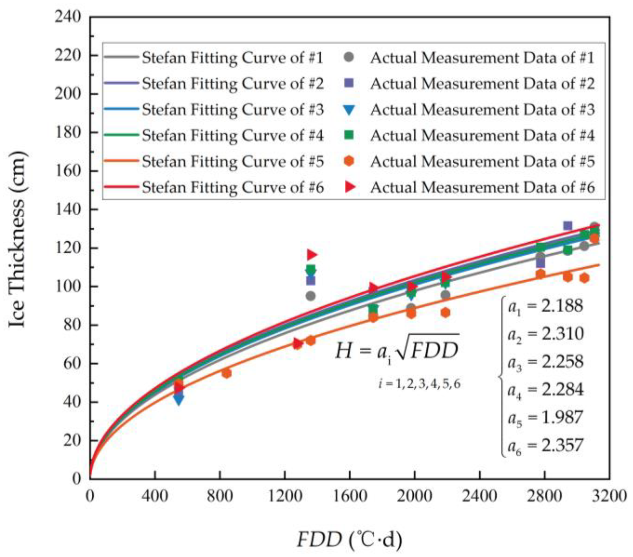
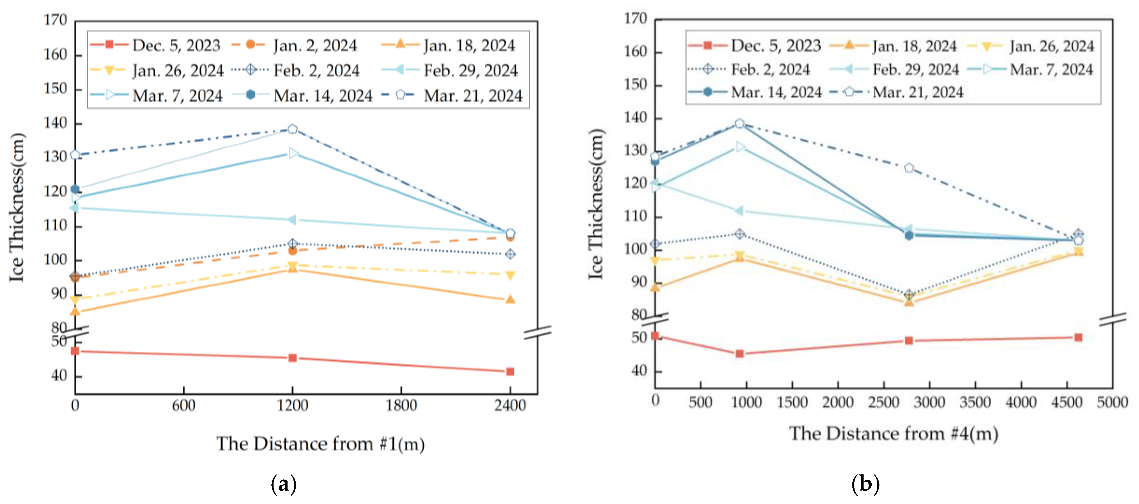
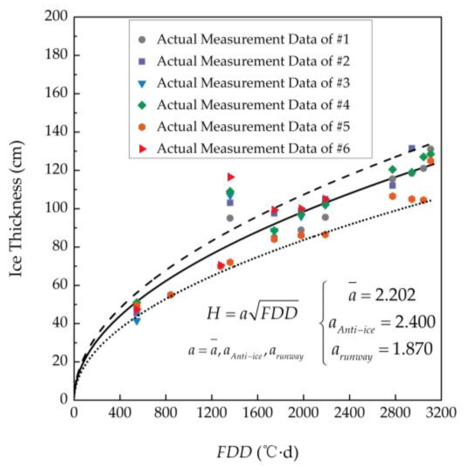
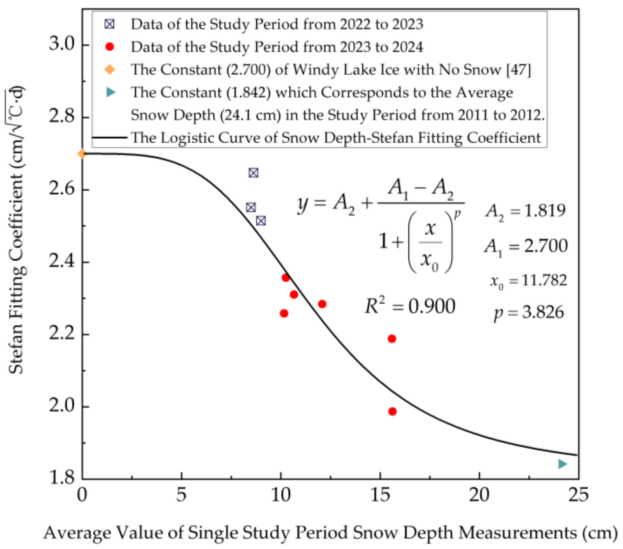
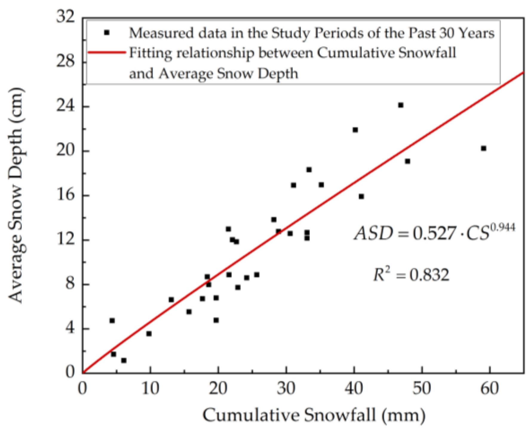
4. Measurement of Ice Thickness Distribution and Its Relationship with Negative Accumulated Temperature

The growth and melting of lake ice mostly rely on temperature and the accumulation of snow on the ice surface. Winter snowfall in Chen Barag Banner affects the processes of lake ice growth and melting. One of the simplest evaluation methods is the mathematical model that relates ice thickness with negative accumulated temperature throughout the ice growth period, known as the degree-day model [17,18,19,20]. The statistical coefficient indicates the influence of snow cover, local hydrology, geographical information, and other factors. The Chen Barag Banner meteorological station recorded a daily mean temperature below 0 °C on 30 October 2023, which began to rise above 0 °C on 27 March 2024. Thus, the negative accumulated temperature at the Chen Barag Banner meteorological station over the study period from 2023 to 2024 may be calculated. Huhenuoer Lake ice is mainly constituted of a columnar-grained ice layer. The wetness of the snow is not significant, and the impact of wind erosion on the snow is limited. We performed six measurements of ice thickness between 5 December 2023 and 21 March 2024. We collected ice thickness data from six sites (#1–#6), as depicted in Figure 4. Table 3 displays the measurements of ice thickness and snow depth collected by drilling holes in Huhenuoer Lake during the study period from 2023 to 2024. The data in Table 3 are stored as integers. We use them to analyze the ice-growing process at each site.
This section provides further analysis using a model for ice growth. In the end, we decided to use the Stefan model.
The reason for selecting this approach is to achieve an acceptable compromise between technical ease of use and safety. The Stefan model expression is simple to understand and user-friendly. There is limited literature regarding the application of this strategy to ice runway design, but the subsequent analytical method employs various levels of safety factors to ensure safety.
Stefan developed an analytical formula for calculating ice thickness in 1891 [21]. The surface temperature of the ice corresponds to the air temperature, while the temperature at the ice bottom aligns with the freezing point. Heat transmission within the ice only aligns with its growth direction and spreads linearly throughout. As a result, the ice thickness varies throughout time.
The Stefan model can be shown as follows:
H i = a F D D
where Hi is the ice thickness, and FDD is cumulative freezing degree days. The FDD, also known as the sum of negative degree days, provides the cumulative total of below-zero temperatures for each day that follows, making the calculation for determining ice thickness simpler [22]. a represents Stefan’s coefficient in the degree-day approach. It relates not only to the physical characteristics of ice but also to the average depth of snow above the ice.
Ice analysis extensively uses the previously mentioned Stefan equation. Subsequently, we plan to describe the application of the Stefan equation within this investigation. For the fitting operation, we exclude the measurements of ice thickness (H) values from the six sites (i.e., #1–#6) where ice growth has reached the lake bottom. Then, the measured ice thickness and negative accumulated temperature by the freezing degree day (FDD) are fitted using the Stefan curve, resulting in the respective statistical coefficients for the six sites. Figure 5 displays the Stefan fitting results for the six sites.
Figure 5 illustrates variations of ice thickness at various places throughout the lake. To describe the findings about the ice thickness at different times more clearly, we created an ice thickness diagram indicating the relative distance from sites #1 (the route oriented towards #1–#2–#3) and #4 (the route oriented towards #4–#2–#5–#6), with the findings shown in Figure 6.
Table 3 indicates that during the initial phase (2 January 2024), ice formations developed more quickly in the southern region than in the northern region, with a small area of thin ice present in the lake’s center. During the subsequent period (21 March 2024), the ice in the southern region of the lake grew slowly and even touched the lake bottom due to the shallow water conditions. Conversely, the ice in the northern section of the lake was comparatively thick.

5. Feasibility Analysis of Huhenuoer Lake Ice as a Temporary Runway

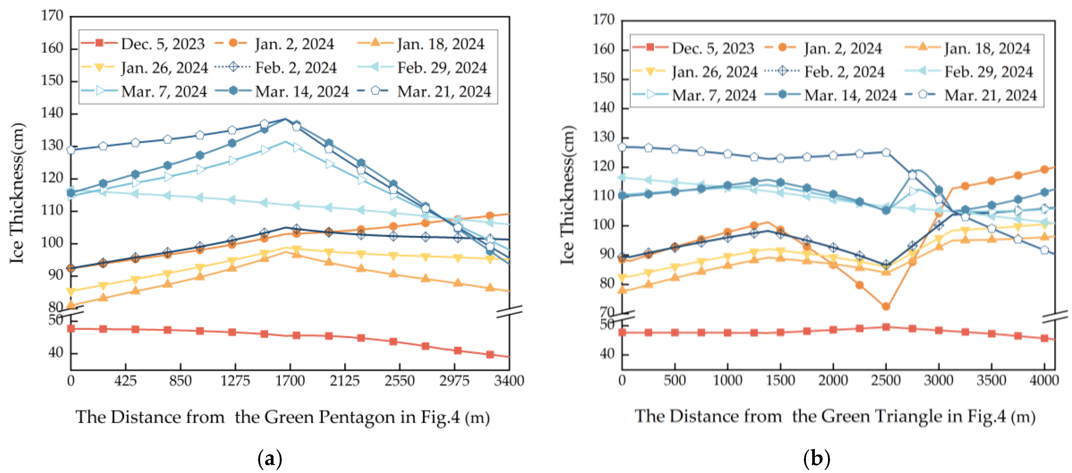
5.1. The Runway Position and Ice Thickness Distribution

Analysis of wind speed and direction data at the Chen Barag Banner meteorological station from 1993 to 2023 indicates that the optimal runway orientations for the Huhenuoer Lake temporary airport are 90–270° and 130–310°. Given that the water in the southern region of Huhenuoer Lake is shallow and the ice in the central area is thin, we utilize the 90–270° line and the 130–310° line to identify the broadest location in the northern section of the lake as the proposed runway position. The distances between the two lakesides measured in this way are 3400 m and 4100 m, respectively.
Due to the low friction coefficient of the ice runway, it is necessary to maximize its length. Additionally, the surface of the ice runway may be covered with a layer of compacted snow, as in the case of the Pegasus runway [4], to mitigate melting caused by solar radiation and other factors. Consequently, based on the assumption that the landing distance of a compacted snow runway requires not less than 1.6 times the length of a land runway [6], the 3400 m length of Huhenuoer Lake ice is comparable to approximately 2000 m of a land runway, which is suitable for the takeoff and landing of lightweight aircraft. The C130 requires a land runway length of 1830 m for ground operations. Without a complete examination of the ice thickness, the ice of the northern part of Huhenuoer Lake is capable of supporting the takeoff and landing of aircraft weighing less than the C130, ensuring safety.
Figure 7 identifies two envelope lines, showing the upper- and lower-limit envelopes of ice thickness throughout the study period of 2023–2024 at Huhenuoer Lake. Different research backgrounds, including purposes and locations, require the adoption of different envelopes. Previous research has applied similar concepts across different fields [23]. This study indicates that adopting the lower envelope (i.e., a = 1.870) implies the presence of some safety redundancy. This is safe for the design of ice runways.
Figure 7 illustrates that the Stefan coefficient of Huhenuoer Lake ice is 2.202. The coefficient for the upper envelope is 2.400, while that for the lower envelope is 1.870. For the design of anti-ice structures, such as the anti-ice design of a bridge pier over a reservoir in cold regions studied in reference [24], the upper-bound envelope considered safe for the project should be used. We construct the airport runway on ice to support the aircraft’s weight and withstand the dynamic loads during takeoff and landing. The lower-limit envelope, whose fitting coefficient of ice thickness–negative accumulated temperature is 1.870, should be chosen in accordance with the engineering safety criteria.
The survey on ice surface variation has not been carried out, and theoretically, it will not exceed the magnitude of ice thickness variation.
Based on our newly established route, the thickness variation can be assessed as follows:
  • The non-uniformity should be minimized, where non-uniformity = (maximum ice thickness along the route − minimum ice thickness along the route)/maximum ice thickness along the route.
  • The maximum change rate should be minimized, where the maximum change rate refers to the highest value of non-uniformity per unit length over the entire route.
Table 4 presents the ice thickness values for the 90–270° and 130–310° routes, calculated using interpolation, allowing for the assessment of non-uniformity and the maximum change rate of ice thickness for both routes.
We show the variation in ice thickness for the two routes at each ice measuring time using an interpolation method. The results are shown in Figure 8.
Under adverse conditions, assuming that the ice temperature is higher than −9 °C and that all of the aircraft are wheeled, the necessary lake ice thickness may be determined by calculating for the various aircraft types [5,25,26,27,28,29,30]. Next, we can determine the beginning of the fundamental time using the negative accumulated temperature associated with the lake ice thickness and designate 26 March 2024 as the end of the fundamental period.
From a safety point of view, the ice thickness may change before and after the operational period. This means that dividing the length of the fundamental period by the safety factor (set at 1.5 in this study) gives us the conservative operational period for the aircraft during the winter, assuming that the middle time point of both the fundamental and conservative periods is the same. Blaisdell et al. indicate that the safety factor for ice runways should be a minimum of 1.25 and a maximum of 1.5 [4]. A safety factor beyond 1.5 diminishes confidence in the runway’s capacity to support aircraft. This section establishes the safety factor at 1.5. At the same time, we also observe that in [4], tire pressure has a safety factor of 1.6 for a specific configuration. The Stefan coefficient has been established as 1.870 in this section. The fitted Stefan coefficient is 2.202, resulting in a calculation of 1.5 × 2.202/1.870 = 1.77, which exceeds 1.6.
We can mitigate the inaccurate prediction of the ice formation and melting process to the greatest extent feasible regarding operational duration, thereby addressing the deficiency in ice thickness. Using the study period from 2023 to 2024 as an example, Figure 9 can be developed by displaying the data of different aircraft.
Table 5 presents the above findings in more detail.
Table 5 indicates that small aircraft like the An-2 will have approximately 85 conservative days during the study period of 2023–2024. However, as aircraft weight increases, the conservative operational period will progressively diminish, making it unsuitable for large transport aircraft such as the C-17. Appendix B [31,32,33,34] shows the required ice thickness and runway length associated with the maximum landing weight of other aircraft.

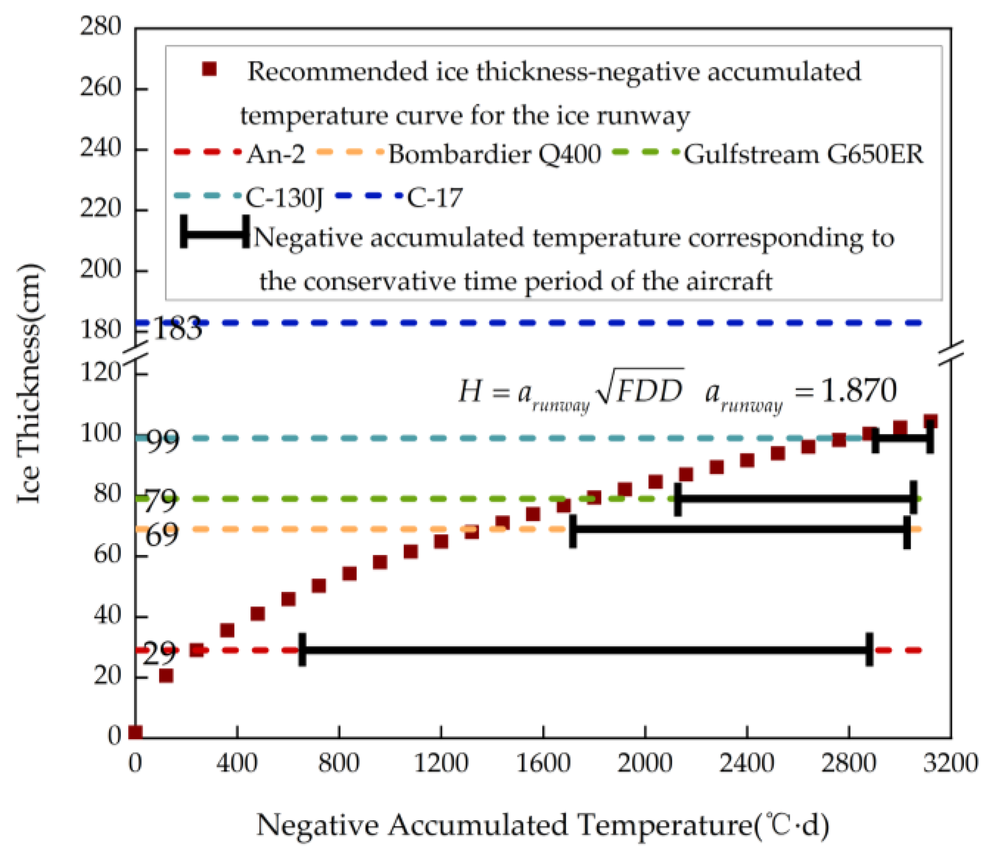
5.2. Feasibility of Using Huhenuoer Lake Ice as the Temporary Runway Every Winter in the Future

In the research period of 2023–2024, a fitting Stefan coefficient of 1.870 may be used to assess the relationship between ice thickness and negative accumulated temperature, supporting the evaluation of ice thickness on various days for the takeoff and landing of different aircraft types. Will we be able to use this coefficient for assessment in future study periods? The assumption is impractical theoretically. The variation of snow depth on the ice surface of Huhenuoer Lake each year affects ice formation differently. This impact is seen in the magnitude of the Stefan coefficient in the relationship between ice thickness and negative accumulated temperature. Generally, a thinner layer of snow corresponds to a higher Stefan coefficient, and vice versa.
Given the above-mentioned impact of snow on the Stefan coefficient, the following will go over how to ascertain the scientific relationship between the two variables. If the snow depth varies, we must use statistics to determine the value of coefficient A. Given that the latitude of Hongqi Pao Reservoir closely resembles that of Huhenuoer Lake (Hongqi Pao Reservoir at 46°36′ N and Huhenuoer Lake at 49°18′ N) [35,36], we refer to Wang’s study of Hongqi Pao Reservoir to determine the Stefan coefficient under conditions of maximum snow depth. Wang investigated the empirical formula that identifies the correlation between the thickness of the ice sheet and the negative accumulated temperature beneath the snow cover in Hongqi Pao Reservoir [37]. We note that the average snow depth at Huhenuoer Lake during the 2011–2012 study period reached 24.1 cm, the highest recorded in the past three decades. Through a fitting procedure, we obtain a Stefan coefficient of 1.842 from the Zubov model data [37], which corresponds to a snow depth of 24.1 cm. Using the logistic fitting method, we can find the link between the depth of the snow and the Stefan coefficient at Huhenuoer Lake by combining data from all study sites during the study periods of 2022–2023 and 2023–2024, along with data from other sources [38] that show the Stefan coefficient of windy lake ice with no snow to be 2.700. The primary advantage of this statistical formula is its ability to show that the Stefan coefficient corresponds to the values reported in the literature under bare ice conditions while also indicating that it diminishes as snow depth increases, up to a certain limit. The results are shown in Figure 10.
The Chen Barag Banner meteorological station has historically recorded winter snowfall, but it does not record the depth of the snow on the ice surface. How do we measure the depth of snow? This research employs a statistical analysis of the cumulative snowfall and snow depth during the negative accumulated temperature statistical period recorded by the Chen Barag Banner meteorological station. The low temperature and high humidity in Chen Barag Banner, Inner Mongolia, lead to the conclusion that snow undergoes a natural metamorphism process without sublimation. Figure 11 shows a fitting method that can only be used to model the relationship between cumulative snowfall and average snow depth over the study period of the last 30 years in Chen Barag Banner. With an R2 value of 0.832, this method is good for modeling this relationship.
Following these operations, the correlation among ice thickness, negative accumulated temperature, and cumulative snowfall for the temporary runway at Huhenuoer Lake can be expressed as indicated in Equation (2):
H i = 1.819 + 2.700 1.819 1 + 0.527 C S 0.944 11.782 3.826 F D D = 1.819 + 0.881 1 + C S 3.612 145491.141 F D D
where CS is the cumulative snowfall. Can the findings obtained during the study period of 2023–2024 be applicable in the winter of the following 10, 15, 20, 25, or even 50 years? How should we assess the return period? In the return period analysis, although global warming cannot be included, the existing meteorological data already contain information from the time of climatic warming. Moreover, the ice thickness, influenced by harmful climatic circumstances, with a return period of 50 years, could serve as a criterion for other winters that do not exceed 50 years.
The Pearson type three (P-III) distribution curve technique [39,40,41,42,43,44,45,46], often used in hydrometeorological studies, is utilized to derive the P-III distribution curve of cumulative snowfall during the study periods of the last 30 years in Chen Barag Banner, shown as Figure 12. Please refer to Appendix C for details of the P-III method.
A similar P-III distribution analyzes the negative accumulated temperature at the Chen Barag Banner meteorological station during winter for the same time, as shown in Figure 13.
Equation (2) indicates that increased cumulative snowfall results in impacts on the ice becoming thinner, with the 2% frequency in Figure 12 denoting an occurrence once every 50 years. As for FDD, a frequency of 98% in Figure 13 is used to denote the 50-year return period, while Table 6 is designed based on the combination of the thick snow layer on the ice surface and the low negative accumulated temperature throughout various return periods.
We insert the input values into Equation (2), which establishes a relationship between cumulative snowfall, negative accumulated temperature, and ice thickness. This connection allows us to calculate the ice thickness throughout various return periods. We can determine the take-off and landing periods for different aircraft types during different return periods by combining the ice thickness calculated by Equation (2) with the minimum ice thickness required for different aircraft types, taking into account the longest temporary runway length. The most adverse effect of combination might serve as the minimal use period during the planning stage of a temporary airport runway.

6. Conclusions and Suggestions

This paper develops six fixed ice thickness monitoring sites based on limited measurements of ice thickness during the study period of 2022–2023, considering the meteorological data near Huhenuoer Lake and the feasibility of utilizing it as a temporary take-off and landing runway, in accordance with the general characteristics of lake ice thickness distribution. The ice thickness was measured at different times throughout the study period of 2023–2024 at the six sites. The actual requirements of the runway, along with the measured data regarding length, ice thickness, and service period of the temporary runway, as well as the analysis of various return periods, demonstrate the feasibility of the Huhenuoer Lake ice supporting a temporary runway during different winter periods. The specific conclusions are as follows:
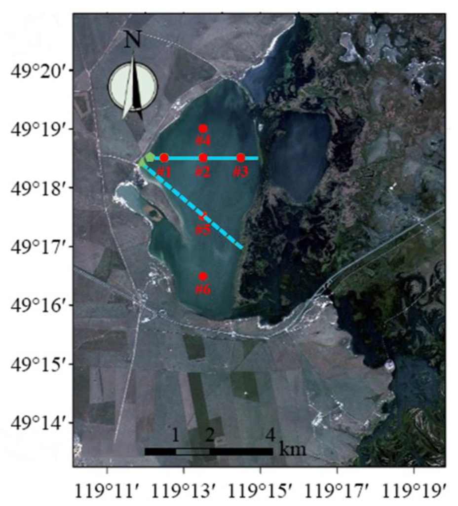
  • Investigations have shown that the ice in the lake’s center is thin, particularly in the southwest of Huhenuoer Lake. Furthermore, the southern region of Huhenuoer Lake is shallow, and in this region, the lake ice can reach the bottom of the lake. The northern section of Huhenuoer Lake may serve as the temporary take-off and landing runway for aircraft on the lake ice during winter.
  • The 30-year historical data on wind speed and direction from the Chen Barag Banner meteorological station near Huhenuoer Lake indicate the predominant wind direction and frequency throughout the winter ice season in this region. The criteria requires a 95% usability factor for aircraft takeoffs and landings in wind conditions, unaffected by crosswinds. The aircraft’s runway orientations on the Huhenuoer Lake ice are 90–270° and 130–310°.
  • In the northern section of the lake, the straight-line distances of 90–270° and 130–310° indicate that the greatest lengths are 3400 m and 4100 m, respectively. Due to the low friction coefficient of an ice surface, the recommended length of an ice runway with a compacted snow layer is 1.6 times that of land. The minimum operational runway length for Huhenuoer Lake is established at 3100 m. Considering the requirements of maximum ice thickness and irregular ice distribution, it is capable of facilitating the takeoff and landing of aircraft such as the C130.
  • We establish the fitting relationship between ice thickness, negative accumulated temperature, and cumulative snowfall at Huhenuoer Lake, using the safety of aircraft takeoff and landing as an engineering design requirement. We provide the designated service period for takeoff and landing for several aircraft types. An analysis of the shortest application period for the next 50 years is conducted.
This workprovides a comprehensive examination of aircraft takeoffs and landings at Huhenuoer Lake. However, there are parts that require enhancement and supplementation. We recommend that future field investigations and studies incorporate the following components:
  • The findings of this article provide support for the design of ice aircraft takeoff and landing at Huhenuoer Lake; nonetheless, a comprehensive survey is necessary for practical implementation. This research suggests that the northern region of Huhenuoer Lake should be the primary location for a limited number of ice thickness monitoring sites, due to the thick ice, low temperatures, and challenges associated with field operations.
  • For the potential runway ice and compacted snow layer, it is crucial to evaluate not only the variability in ice thickness on the proposed runway but also the undulations of the ice surface. Additionally, it is crucial to conduct research aimed at enhancing the friction coefficient and minimizing surface undulation of the compacted snow.
  • The investigation assessing the bearing capability of the temporary ice runway at Huhenuoer Lake will be integrated into the field of ice engineering. The effective maintenance of the ice runway is in the construction and application stages. It requires measurement of not only ice thickness but also mechanical characteristics, including ice bending strength, elastic modulus, Poisson’s ratio, and compressive strength. Therefore, in order to implement the ice runway, it is crucial to conduct experimental research on the physical characteristics of the ice layer during future investigations of Huhenuoer Lake.
  • The Stefan model employed in this research is user-friendly, and various ice thickness models, such as the Ashton model [47,48], are also appropriate for ice runway construction. This represents a significant area for future investigation.

Author Contributions

Conceptualization, P.L.; methodology, Q.Z. and P.L.; investigation, Y.W., Q.W. (Qingjiang Wang) and Q.W. (Qingkai Wang); data curation., B.Z. and X.B.; formal analysis, Q.Z., Q.W. (Qingjiang Wang) and Q.W. (Qingkai Wang); visualization, Y.W., Q.W. (Qingjiang Wang) and Q.W. (Qingkai Wang); writing—original draft preparation, Q.Z. and J.H.; writing—review and editing, Y.W., B.Z., P.L. and X.B.; project administration, Y.W.; funding acquisition, Y.W. All authors have read and agreed to the published version of the manuscript.

Funding

This work was supported by a project of the Inner Mongolia Autonomous Region Natural Science Foundation (grant number 2023MS04006).

Data Availability Statement

The original contributions presented in the study are included in the article; for a more detailed data request, please contact the corresponding author directly.

Conflicts of Interest

The authors declare no conflicts of interest.

Appendix A. Beginning Time, Ending Time, Days, Negative Accumulated Temperature, and Cumulative Snowfall for Each Research Period from 1993 to 2023

NumberBeginning TimeEnding TimeDaysNegative Accumulated
Temperature (°C·d)
Cumulative Snowfall (mm)
1993–199428 October 199329 March 19941522749.229.5
1994–19956 November 199427 March 19951412211.213.6
1995–199629 October 19955 April 19961592511.219.7
1996–199723 October 199625 March 19971533009.930.6
1997–199820 October 199725 March 19981562509.217.7
1998–199930 October 19985 April 19991572746.421.6
1999–200020 October 19996 April 20001693228.847.9
2000–20012 November 20003 April 20011523150.815.7
2001–200230 October 200110 March 20021312367.522.6
2002–200317 October 200229 March 20031633076.224.2
2003–20041 November 200325 March 20041452811.328.2
2004–20054 November 20041 April 20051482869.322.1
2005–20066 November 200531 March 20061452811.228.9
2006–20074 November 20066 April 20071532770.833.1
2007–200825 October 20077 March 20081342524.613.1
2008–200923 October 20081 April 20091602858.541.1
2009–20106 November 200917 April 20101623249.335.2
2010–20116 November 20102 April 20111473016.140.2
2011–20122 November 201127 March 20121463433.646.9
2012–201327 October 201219 April 20131743490.759.1
2013–20145 November 201322 March 20141372519.533.4
2014–201530 October 201424 March 20151452474.325.7
2015–201614 November 201519 March 20161262636.318.6
2016–201717 October 201627 March 20171612837.521.5
2017–201828 October 201723 March 20181463072.418.4
2018–20193 November 201816 March 20191332135.04.4
2019–20201 November 201923 March 20201432739.919.7
2020–202112 November 202012 March 20211202263.04.6
2021–20224 November 20218 March 20221242344.99.8
2022–202331 October 202227 March 20231472766.322.9
2023–202430 October 202326 March 20241483135.034.9

Appendix B. The Maximum Landing Weight (MLW) for Some Aircraft Types, the Needed Ice Thickness, and the Needed Length on an Ice Runway (Covered with Compacted Snow)

Aircraft TypesThe MLW (t)Needed Ice Thickness (cm)Needed Length on Ice Runway Covered with Compacted Snow (m)
CZAW SportCruiser LSA0.610200
Cessna 172N113470
Cessna Caravan4241000
Cessna Citation CJ4 Gen27341660
Saab 34013462060
Bombardier CRJ70030712500
Embraer 17033742630
Bombardier Global Express36772700
ARJ21-70038792720
ERJ 19043843290
Airbus A220-10051922340
Boeing 737-70058982930
Airbus A319neo631022960

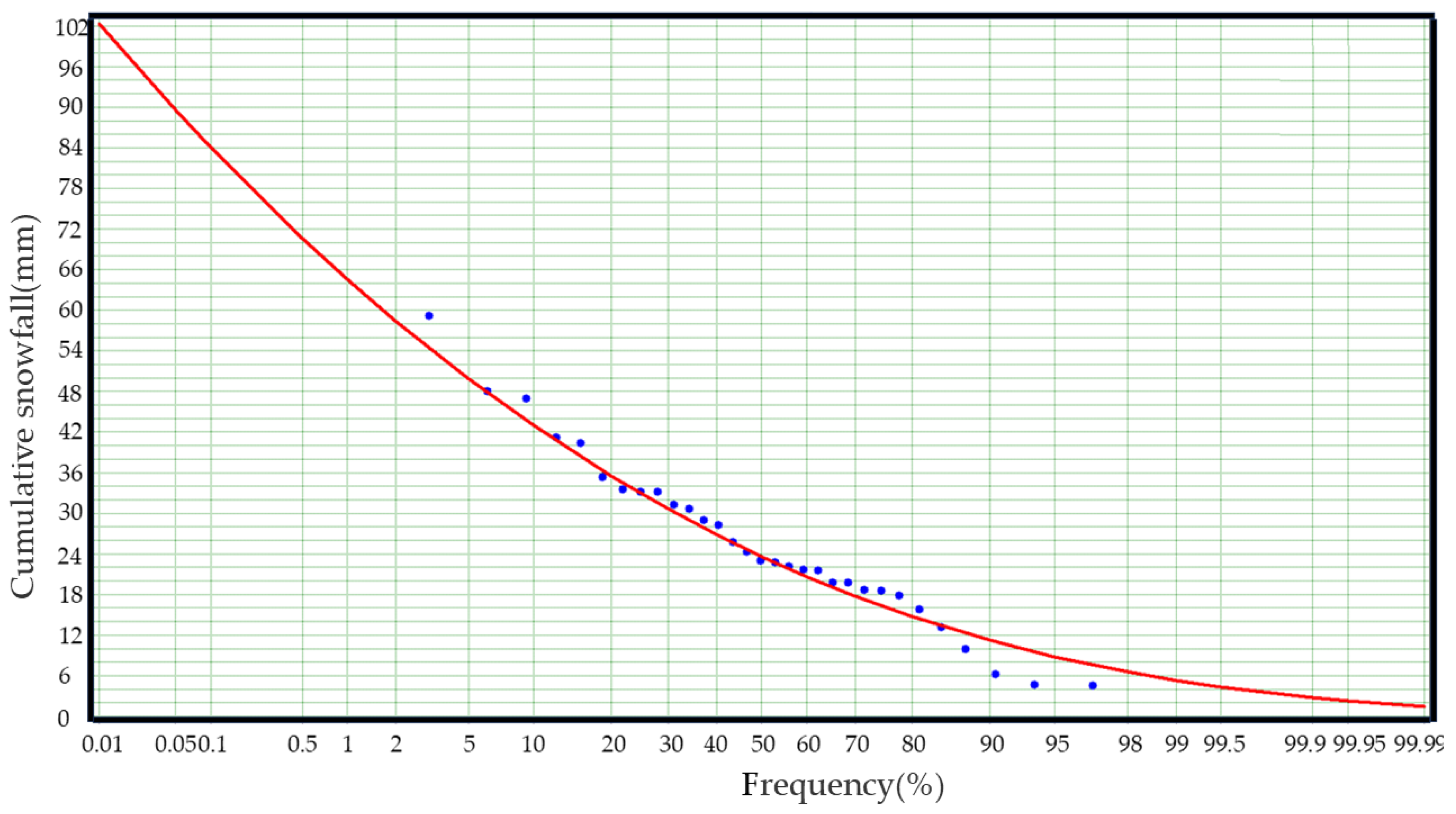
Appendix C. The Details of P-III Analysis

The probability density function of P-III distribution is:
f x = β α Γ α x x 0 α 1 exp β x x 0
where Γ(α) is the gamma function, and α, β, and x0 are the shape, scale, and position coefficients, respectively. Refer to the below for details.
α = 4 / C s 2 β = 2 / x ¯ C v C s x 0 = x ¯ ( 1 2 C v / C s )
where Cs is skewness coefficient, Cv is variation coefficient, and x ¯ is the average.
With a 50-year return period—that is, a frequency of 2%—Figure 12 illustrates the upper-limit cumulative snowfall throughout winter: 58.4 mm. This number represents the maximum snowfall that occurs once every 50 years, with the associated snow cover serving as the greatest limit. Snowfall can negatively impact the minimum ice thickness and limit aircraft operations on ice surfaces. Figure 12 delineates the cumulative snowfall in the study period over return periods of 45 years, 30 years, 25 years, 20 years, 15 years, and 10 years.

References

  1. Abele, G.; Frankenstein, G.E. Snow and Ice Properties as Related to Roads and Runways in Antarctica; US Army Cold Regions Research & Engineering Laboratory: Hanover, NH, USA, 1967; Volume 176. [Google Scholar]
  2. White, G.; McCallum, A. Review of ice and snow runway pavements. Int. J. Pavement Res. Technol. 2018, 11, 311–320. [Google Scholar] [CrossRef]
  3. Masterson, D.M. State of the art of ice bearing capacity and ice construction. Cold Reg. Sci. Technol. 2009, 58, 99–112. [Google Scholar] [CrossRef]
  4. Blaisdell, G.L.; Lang, R.M.; Crist, G.; Kurtti, K.; Harbin, R.J.; Flora, D. Construction, Maintenance, and Operation of a Glacial Runway, McMurdo Station, Antarctica; ERDC/CRREL M-98-1; US Army Corps of Engineers, Engineer Research and Development Center: Washington, DC, USA, 1998. [Google Scholar]
  5. Sharp, R.P. Suitability of ice for aircraft landings. Trans. Am. Geophys. Union 1947, 28, 111–119. [Google Scholar] [CrossRef]
  6. Flight Safety Foundation. Landing Distances. In FSF ALAR Briefing Note; Flight Safety Foundation: Alexandria, VA, USA, 2000. [Google Scholar]
  7. Swithinbank, C. Ice Runways Near the South Pole; ERDC/CRREL R-89-19; US Army Corps of Engineers, Engineer Research and Development Center: Washington, DC, USA, 1989. [Google Scholar]
  8. Squire, V.A.; Robinson, W.H.; Langhorne, P.J.; Haskell, T.G. Vehicles and aircraft on floating ice. Nature 1988, 333, 159–161. [Google Scholar] [CrossRef]
  9. McCallum, A.B. Movement and expected lifetime of the Casey ice runway. In Proceedings of the 13th International Conference on Cold Regions Engineering, Orono, ME, USA, 23–26 July 2006; American Society of Civil Engineers (ASCE): Reston, VA, USA, 2006; pp. 1–19. [Google Scholar]
  10. Editorial Committee of Encyclopedia of Rivers and Lakes in China. Encyclopedia of Rivers and Lakes in China: Section of Heilong River and Liaohe River Basins; China Water & Power Press: Beijing, China, 2014; p. 17. (In Chinese) [Google Scholar]
  11. Lu, J.; Xia, C. Investigation for emphasis cold water domain of inland in China Investigation for the cold water domain and its resources in Neimonggu autonomous region. Chin. J. Fish. 2005, 18, 47–52. (In Chinese) [Google Scholar]
  12. Graf, R. Estimation of the Dependence of Ice Phenomena Trends on Air and Water Temperature in River. Water 2020, 12, 3494. [Google Scholar] [CrossRef]
  13. Mousa, R.M.; Mumayiz, S.A. Optimization of runway orientation. J. Transp. Eng. 2000, 126, 228–236. [Google Scholar] [CrossRef]
  14. Ashford, N.; Wright, P.H. Airport Engineering, 3rd ed.; John Wiley & Sons, Inc: New York, USA, 1992. [Google Scholar]
  15. Sarsam, S.I. Runway orientation problems–A case study of Middle Euphrates International Airport MEIA. In Proceedings of the 2nd International Conference of Buildings, Construction and Environmental Engineering (BCEE2-2015), Beirut, Lebanon, 17–18 October 2015. [Google Scholar]
  16. Haehnel, R.B.; Blaisdell, G.L.; Melendy, T.D.; Shoop, S.; Courville, Z. A Snow Runway for Supporting Wheeled Aircraft: Phoenix Airfield, McMurdo, Antarctica; ERDC/CRREL TR-19-4; US Army Corps of Engineers, Engineer Research and Development Center: Washington, DC, USA, 2019. [Google Scholar]
  17. Lotsari, E.; Lind, L.; Kämäri, M. Impacts of Hydro-Climatically Varying Years on Ice Growth and Decay in a Subarctic River. Water 2019, 11, 2058. [Google Scholar] [CrossRef]
  18. Brooks, R.N. Quantifying Peak Freshwater Ice Across the Northern Hemisphere Using a Regionally Defined Degree-Day Ice-Growth Model. Master’s Thesis, University of Victoria, Victoria, BC, Canada, 2012. [Google Scholar]
  19. Korhonen, J. Long-term changes in lake ice cover in Finland. Hydrol. Res. 2006, 37, 347–363. [Google Scholar] [CrossRef]
  20. Solarski, M.; Rzetala, M. A Comparison of Model Calculations of Ice Thickness with the Observations on Small Water Bodies in Katowice Upland (Southern Poland). Water 2022, 14, 3886. [Google Scholar] [CrossRef]
  21. Stefan, J. Ueber die Theorie der Eisbildung, insbesondere über die Eisbildung im Polarmeere. Ann. Phys. 1891, 278, 269–286, In German. [Google Scholar] [CrossRef]
  22. Leppäranta, M. A review of analytical models of sea-ice growth. Atmos. Ocean 1993, 31, 123–138. [Google Scholar] [CrossRef]
  23. Husselmann, M.L.; Van Zyl, J.E. Effect of stand size and income on residential water demand. J. S. Afr. Inst. Civ. Eng. 2006, 48, 12–16. Available online: https://hdl.handle.net/10520/EJC26987 (accessed on 9 December 2024).
  24. Lin, L. Study on Effect of Ice Deformation on Reservoir Piers. Master’s Thesis, Dalian University of Technology, Dalian, China, 2023. (In Chinese). [Google Scholar]
  25. Schiff, B. Antonov AN-2 The Flying Bear. Available online: https://www.aopa.org/news-and-media/all-news/2001/october/pilot/antonov-an-2 (accessed on 9 December 2024).
  26. Aero Corner. Bombardier Q400. Available online: https://aerocorner.com/aircraft/bombardier-q400/ (accessed on 9 December 2024).
  27. Austrian Airlines. Bombardier Q400. Available online: https://www.austrian.com/nl/en/bombardier-q400 (accessed on 9 December 2024).
  28. GlobalAir.com. Gulfstream G650ER. Available online: https://www.globalair.com/aircraft-for-sale/specifications?specid=1520 (accessed on 9 December 2024).
  29. Rocco. Lockheed C-5 Galaxy vs. Lockheed C-130 Hercules. Available online: https://aerocorner.com/comparison/lockheed-c-5-galaxy-vs-lockheed-c-130-hercules/ (accessed on 9 December 2024).
  30. Ultimate Specs. C-17 Globemaster III Technical Data. 1991. Available online: https://www.ultimatespecs.com/aircraft-specs/boeing/boeing-c-17-globemaster-iii-1991 (accessed on 9 December 2024).
  31. GlobalAir.com. CZAW SportCruiser LSA. Available online: https://www.globalair.com/aircraft-for-sale/specifications?specid=1378 (accessed on 9 December 2024).
  32. GlobalAir.com. Cessna 172N. Available online: https://www.globalair.com/aircraft-for-sale/specifications?specid=1237 (accessed on 9 December 2024).
  33. Textron Aviation Inc. Citation CJ4 Gen2. Available online: https://cessna.txtav.com/citation/cj4-gen2#_model-specs (accessed on 9 December 2024).
  34. English Wikipedia. List of Airliners by Maximum Takeoff Weight. Available online: https://en.wikipedia.org/wiki/List_of_airliners_by_maximum_takeoff_weight#cite_note-27 (accessed on 9 December 2024).
  35. Li, Z.; Fu, X.; Shi, L.; Huang, W.; Li, C. Recent Advances and Challenges in the Inverse Identification of Thermal Diffusivity of Natural Ice in China. Water 2023, 15, 1041. [Google Scholar] [CrossRef]
  36. Shi, L.; Li, Z.; Lu, P.; Feng, E. Influence of ice temperature on thermal diffusivity of natural freshwater ice. J. Hydraul. Eng. 2013, 44, 1112–1117. (In Chinese) [Google Scholar] [CrossRef]
  37. Wang, T. Exploring of the Relationship between Cold Ice Thickness Reservoir of Growth and Negative Accumulated Temperature. Bohai University: Jinzhou, China, 2011. (In Chinese) [Google Scholar]
  38. Shen, H.T.; Yapa, P.D. A unified degree-day method for river ice cover thickness simulation. Can. J. Civ. Eng. 1985, 12, 54–62. [Google Scholar] [CrossRef]
  39. Gu, H.; Yu, Z.; Li, G.; Ju, Q. Nonstationary Multivariate Hydrological Frequency Analysis in the Upper Zhanghe River Basin, China. Water 2018, 10, 772. [Google Scholar] [CrossRef]
  40. Lu, Y. Impacts of Climate Change on Hydrological Hazards: Mechanisms, Predictions and Coping Strategies. Appl. Math. Nonlinear Sci. 2024, 9, 1–17. [Google Scholar] [CrossRef]
  41. Mo, C.; Jiang, C.; Lei, X.; Cen, W.; Yan, Z.; Tang, G.; Li, L.; Sun, G.; Xing, Z. Optimal Scheduling of Reservoir Flood Control under Non-Stationary Conditions. Sustainability 2023, 15, 11530. [Google Scholar] [CrossRef]
  42. Xu, K.; Ma, C.; Lian, J.; Bin, L. Joint Probability Analysis of Extreme Precipitation and Storm Tide in a Coastal City under Changing Environment. PLoS ONE 2014, 9, e109341. [Google Scholar] [CrossRef]
  43. Cui, Y.; Tang, H.; Jin, J.; Zhou, Y.; Jiang, S.; Chen, M. System Structure–Based Drought Disaster Risk Assessment Using Remote Sensing and Field Experiment Data. Remote Sens. 2022, 14, 5700. [Google Scholar] [CrossRef]
  44. Liu, Z.; Yang, H.; Wang, T.; Yang, D. Estimating the annual runoff frequency distribution based on climatic conditions and catchment characteristics: A case study across China. Int. Soil Water Conserv. Res. 2023, 11, 470–481. [Google Scholar] [CrossRef]
  45. Ke, Q.; Jonkman, S.N.; Van Gelder, P.H.A.J.M.; Bricker, J.D. Frequency Analysis of Storm-Surge-Induced Flooding for the Huangpu River in Shanghai, China. J. Mar. Sci. Eng. 2018, 6, 70. [Google Scholar] [CrossRef]
  46. Minh, H.V.T.; Lavane, K.; Lanh, L.T.; Thinh, L.V.; Cong, N.P.; Ty, T.V.; Downes, N.K.; Kumar, P. Developing Intensity-Duration-Frequency (IDF) Curves Based on Rainfall Cumulative Distribution Frequency (CDF) for Can Tho City, Vietnam. Earth 2022, 3, 866–880. [Google Scholar] [CrossRef]
  47. Ashton, G.D. Thin ice growth. Water Resour. Res. 1989, 25, 564–566. [Google Scholar] [CrossRef]
  48. Ashton, G.D. River and lake ice thickening, thinning, and snow ice formation. Cold Reg. Sci. Technol. 2011, 68, 3–19. [Google Scholar] [CrossRef]
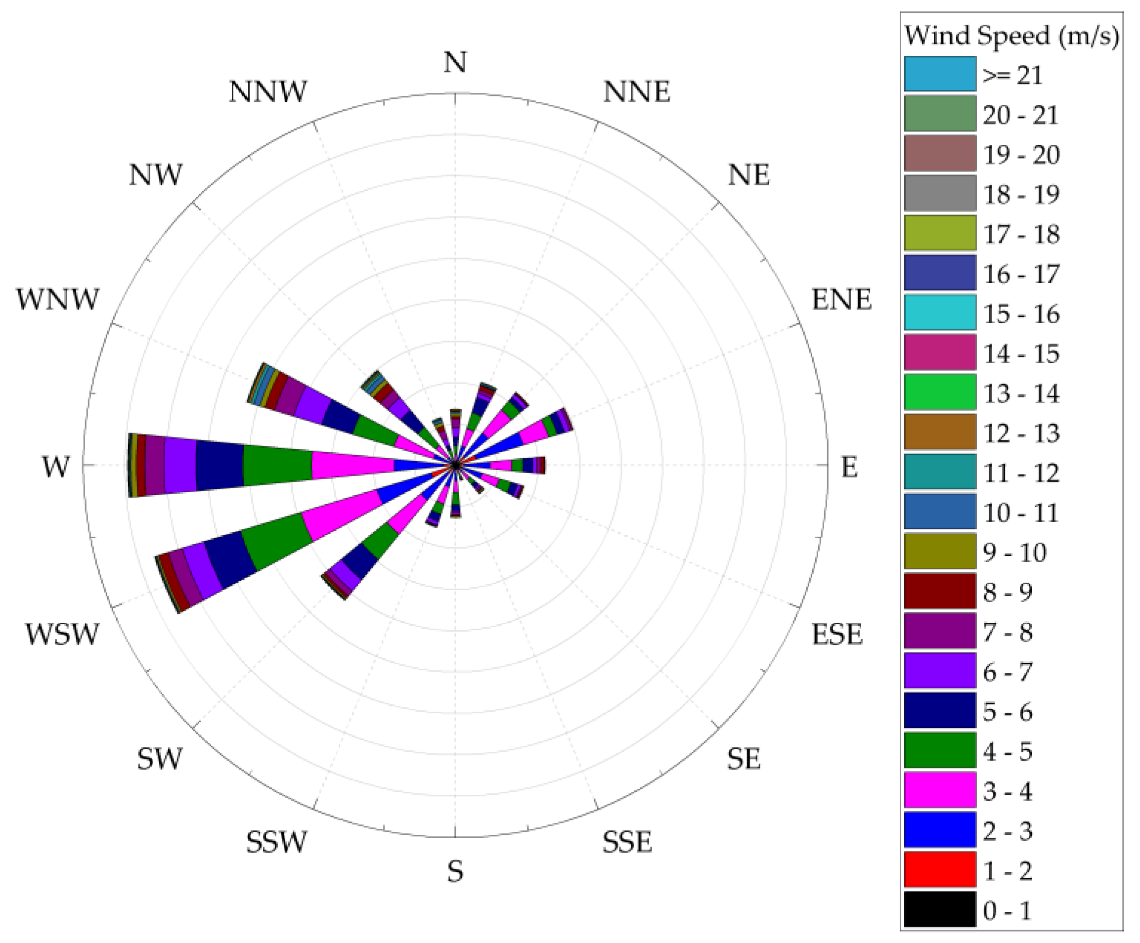
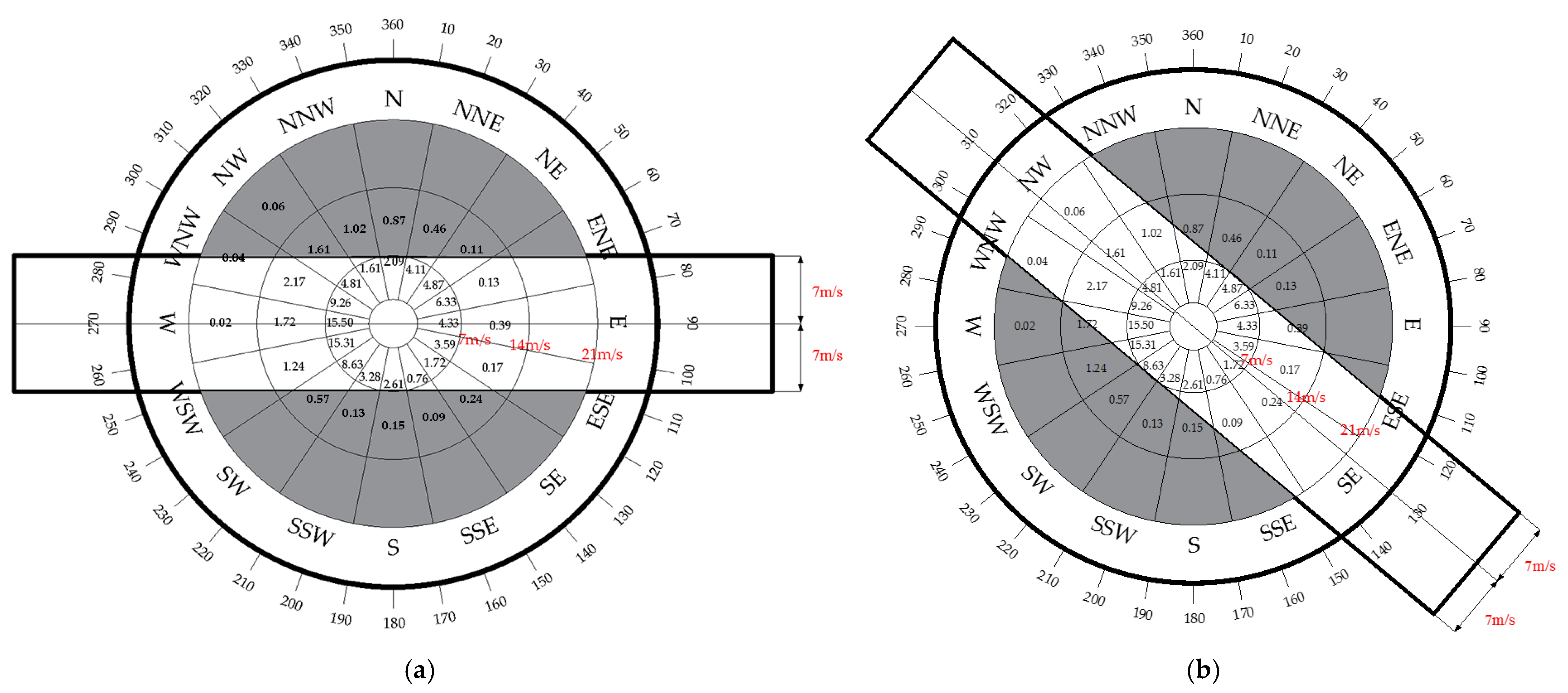
Figure 1. Schematic diagram of the geographical position of Huhenuoer Lake. China is shown in blue on the left, whereas Chen Barag Banner is shown in red. The image on the right displays a high-definition map of Huhenuoer Lake.
Water 17 00400 g001
Figure 2. Wind roses for the 2023–2024 research period at Chen Barag Banner.
Water 17 00400 g002
Figure 3. The wind rose diagram for two arrangements: (a) 90–270°; (b) 130–310°.
Water 17 00400 g003
Figure 4. The high-definition map of the proposed route for the optional ice runway and the ice research sites. The solid line represents the 3400 m scheme oriented from 90–270°, and the starting point on the western side is marked with a green pentagon. The dashed line indicates the 4100 m scheme oriented from 130–310°, and the starting point on the western side is marked with a green triangle.
Water 17 00400 g004
Figure 5. Stefan fitting curves and parameters of negative accumulated temperature and ice thickness of sites #1–#6.
Water 17 00400 g005
Figure 6. Measured ice thickness at six sites at different times: (a) 90–270°; (b) 130–310°.
Water 17 00400 g006
Figure 7. The average Stefan curve (solid line) representing all the ice thickness data from Huhenuoer Lake during the study period of 2023–2024, together with the upper-limit envelope (dashed line) for anti-ice structure design and the lower-limit envelope (dotted line) for ice runway design.
Water 17 00400 g007
Figure 8. Ice thickness of 90–270° and 130–310° runway routes at different measured times: (a) 90–270°; (b) 130–310°.
Water 17 00400 g008
Figure 9. Using the study period from 2023 to 2024 as an example, the Stefan curve depicting the relationship between ice thickness and negative cumulated temperature for Huhenuoer Lake, together with the operating conservative period for each aircraft.
Water 17 00400 g009
Figure 10. Logistic fitting relationship between snow depth and Stefan coefficient of Huhenuoer Lake ice.
Water 17 00400 g010
Figure 11. The relationship between cumulative snowfall and average snow depth over the study period of the last 30 years in Chen Barag Banner.
Water 17 00400 g011
Figure 12. P-III curve representing cumulative snowfall over the study periods of the last 30 years. The blue dots denote the actual data, while the red line illustrates the fitting cumulative snowfall P-III curve for the study period.
Water 17 00400 g012
Figure 13. P-III curve representing negative accumulated temperature over the study periods of the last 30 years. The blue dots denote the actual data, while the red line illustrates the fitting negative accumulated temperature P-III curve for the study period.
Water 17 00400 g013
Table 1. Wind frequency (%) of wind roses used to determine runway orientation in all research periods of Huhenuoer Lake in the past 30 years.
Orientation0~7 m/s7~14 m/s14~21 m/sOrientation0~7 m/s7~14 m/s14~21 m/s
N2.090.87 S2.610.15
NNE4.110.46 SSW3.280.13
NE4.870.11 SW8.630.57
ENE6.330.13 WSW15.311.24
E4.330.39 W15.501.720.02
ESE3.590.17 WNW9.262.170.04
SE1.720.24 NW4.811.610.06
SSE0.760.09 NNW1.611.02
Table 2. The latitude and longitude of Huhenuoer Lake ice survey sites.
Site NumberLongitudeLatitude
#1119°12′30″ E49°18′30″ N
#2119°13′30″ E49°18′30″ N
#3119°14′30″ E49°18′30″ N
#4119°13′30″ E49°19′00″ N
#5119°13′30″ E49°17′30″ N
#6119°13′30″ E49°16′30″ N
Table 3. Ice thickness and snow depth measured by hole-drilling in Huhenuoer Lake during the study period from 2023 to 2024.
Date of MeasurementSnow Depth (cm)Ice Thickness (cm)
#1#2#3#4#5#6Average Value
5 December 20231348464251504848
15 December 202315 55 55
29 December 202319 707171
2 January 2024189510310710972117101
18 January 20242085988989849991
26 January 202419899996978610095
2 February 2024209610510210287105100
29 February 202422116112108121107103111
7 March 202421119132108119105103114
14 March 202419121139108127105103117
21 March 202416131139108129125103123
Table 4. The maximum value of the ice thickness, non-uniformity, and change rate of ice thickness for runway routes 90–270° and 130–310° at different times.
Date of MeasurementRunway OrientationIce Thickness
on The Route (cm)
Non-Uniformity (%)Maximum Change Rate (‰)
Min Value Max Value
5 December 202390–270°394818.2−0.1
130–310°45508.5−0.0
2 January 202490–270°9210915.40.1
130–310°7212039.70.7
18 January 202490–270°819816.90.1
130–310°789619.10.2
26 January 202490–270°859913.60.1
130–310°8310118.20.2
2 February 202490–270°9210512.00.1
130–310°8710618.40.3
29 February 202490–270°1061179.1−0.0
130–310°10111713.4−0.1
7 March 202490–270°9813225.4−0.2
130–310°1051148.0−0.3
14 March 202490–270°9413932.4−0.3
130–310°10511911.8−0.6
21 March 202490–270°9613931.0−0.3
130–310°9012728.9−0.3
Table 5. Using the research period from 2023 to 2024 as an example, the conservative operational period of different aircraft types and the necessary length of the ice runway are assessed. The needed length of the ice runway is 1.6 times the greater of the aircraft’s take-off distance and landing distance.
Aircraft TypeMaximum Landing Weight (t)Start of the Conservative PeriodEnd of the Conservative PeriodConservative Period (d)Needed Length (m)
An-2710 December 20234 March 202485400
Bombardier Q4002917 January 202412 March 2024552240
Gulfstream G650ER3831 January 202415 March 2024443070
C-130J595 March 202423 March 2024182520
C-172033780
Table 6. The values of cumulative snowfall and negative accumulated temperature from the P-III curve, together with the corresponding ice thickness over various return periods.
Return Periods (Years)Value of the Corresponding Return Period by Cumulative Snowfall P-III Curve (mm)Value of the Corresponding Return Period by Negative Accumulated Temperature P-III Curve (°C·d)
5058.42092.5
4557.52105.5
3053.72158.7
2552.02184.3
2049.92217.0
1547.02262.1
1043.03577.4
Disclaimer/Publisher’s Note: The statements, opinions and data contained in all publications are solely those of the individual author(s) and contributor(s) and not of MDPI and/or the editor(s). MDPI and/or the editor(s) disclaim responsibility for any injury to people or property resulting from any ideas, methods, instructions or products referred to in the content.

