Article

Reconstruction of Daily Runoff Series in Data-Scarce Areas Based on Physically Enhanced Seq-to-Seq-Attention-LSTM Model

1
Institute of Science and Technology, China Three Gorges Corporation, Beijing 101199, China
2
Three Gorges Cascade Dispatch and Communication Center, China Yangtze Power Co., Ltd., Yichang 443000, China
3
China Institute of Water Resources and Hydropower Research, Beijing 100038, China
*
Author to whom correspondence should be addressed.
Water 2025, 17(23), 3396; https://doi.org/10.3390/w17233396
Submission received: 8 September 2025 / Revised: 12 November 2025 / Accepted: 17 November 2025 / Published: 28 November 2025
(This article belongs to the Special Issue Catchment Ecohydrology)

Abstract

With the advancement of remote sensing-based river discharge monitoring in data-scarce regions, reconstructing daily streamflow series from remote sensing data has become a critical hydrological challenge. To address the sparsity of remote sensing inversions and the discontinuity of discharge observations, we propose a physics-enhanced deep learning model—Physics-enhanced Seq-to-Seq Attention LSTM (PSAL)—to achieve high-accuracy daily streamflow reconstruction. The model incorporates input structures aligned with hydrological mechanisms, providing a physically meaningful basis for interpretability and enabling physics-guided learning. Results show that (1) PSAL achieves high reconstruction accuracy across five representative gauging sites on the Jinsha River (mean NSE = 0.81). Among lagged output configurations from T-1 to T-7 days, the T-7 setting yields the best performance (mean NSE = 0.85). (2) Compared with a baseline Seq-to-Seq Attention LSTM model without physics-enhanced features, PSAL significantly improves reconstruction skill (mean ΔNSE = 0.76). Feature ablation analysis further reveals that precipitation, as a key driver of runoff, has a strong influence on model performance (mean ΔNSE = 0.32). This study presents a novel approach that integrates physical knowledge with data-driven methods for streamflow reconstruction in remote sensing-dominated, data-scarce regions, offering theoretical support and methodological guidance for digital twin watershed development and historical hydrological data infilling.

1. Introduction

1.1. Current Research Status of Remote Sensing Runoff Monitoring

In recent years, the continuous advancement of remote sensing technologies has provided unprecedented spatiotemporal coverage for hydrological information acquisition. Traditional ground-based monitoring networks often suffer from spatial unevenness and temporal data gaps, whereas remote sensing, with its wide-area observation and periodic repeatability, demonstrates great potential for monitoring hydrological variables at the basin scale [1]. This is particularly valuable in regions with complex terrain or limited infrastructure, where in situ hydrological monitoring is extremely challenging and remote sensing has become a feasible alternative data source [2]. However, due to the sparse temporal resolution and limited data quality of remote sensing products, remotely sensed streamflow data typically exhibit discontinuities and sparsity [3].
Historically, remote sensing imagery has suffered from sparse temporal coverage and low data quality. Although modern remote sensing technologies now offer high temporal and spatial resolution (e.g., GF-2 with 2-m resolution) [4], data availability during earlier periods—such as from the late 20th to early 21st century—was significantly lower. During the 1980s, advancements in remote sensing, such as the launch of Landsat-4 with 30-m resolution, increased its applications; however, revisit cycles still exceeded 10 days [5]. Notti [6] noted that long revisit intervals hinder the ability of remote sensing to capture continuous records of river flow. In addition, cloud cover—especially during the rainy season—can obstruct optical imagery, limiting its effectiveness in identifying flood extents and compromising the spatial completeness of runoff monitoring [6]. Data quality issues also pose challenges, such as the 2003 Landsat 7 SLC failure, which resulted in approximately 22% of the imagery being affected by data gaps (“black stripes”) [7]. These limitations reduce the amount of usable data and complicate accurate information extraction from remote sensing sources.
These issues result in streamflow records obtained from remote-sensing-based monitoring being markedly sparse and discontinuous. Because such monitoring relies directly on satellite observations [6], it is affected by revisit cycles, cloud and precipitation interference, and fluctuations in data quality. Consequently, streamflow time series derived from historical remote sensing data are often uneven in their spatiotemporal distribution and contain information gaps. This severely restricts its further application in hydrological simulation, especially when calculating the relatively scarce hydrological information from the 1970s to the 1990s. Reconstructing hydrological data for historical periods from remote sensing imagery is therefore of substantial practical significance: providing hydrological background conditions prior to the rapid economic development that began in the late twentieth and early twenty-first centuries will help assess the impacts of human activities and climate change on water resources and supply foundational data for the design of large hydraulic projects [6].

1.2. The Current Situation of Daily Scale Runoff Data Reconstruction

Streamflow data at different temporal scales serve distinct research and management functions in water resources planning and regulation. In terms of dynamic drought threshold setting and establishment of ecological response indicators, daily-scale data are particularly important and possess irreplaceable functions [8]. However, from the late twentieth to the early twenty-first century, the scarcity of gauging stations and limited monitoring capacity led to significant gaps in daily streamflow time series. Against this backdrop, remote sensing, with its broad spatiotemporal coverage, offers a new pathway for efficient and accurate inference of historical hydrological series.
By temporal resolution, streamflow data can be classified into annual, monthly, daily, and hourly scales. Annual-scale data, owing to their long time horizon, are commonly used for overall water resources assessment [9] and macro-scale analyses such as climate change trends [10]; monthly-scale data are widely applied to intra-annual water resources operations, agricultural irrigation planning, and watershed water balance analyses [11]; hourly-scale data typically rely on automated monitoring systems and suit applications with stringent real-time requirements, including flood early warning, storm response, and urban inundation [12]. In contrast, daily-scale streamflow data, which balance timeliness and stability, are the most commonly used in hydrological modeling and engineering management, with broad applications in flood forecasting, water supply system design, agricultural irrigation management, and environmental impact assessment [8]. Moreover, many annual and monthly datasets are aggregated from daily records [7,11]; numerous data-driven hydrological models (e.g., LSTM, GRU) also adopt the daily scale as the modeling unit to continuously simulate watershed responses [13]. Therefore, daily data not only bridge long-term trends and short-term response processes but also constitute the core foundation supporting hydrological process modeling and management decision-making.
In data-scarce regions, uneven distribution of gauging stations and gaps in time series have long impeded studies of daily streamflow, hindering digital modeling of hydrological processes. To address this, researchers have explored a range of methods for reconstructing daily streamflow, which can be broadly categorized into physically based (model-driven) and data-driven approaches.
On one hand, physically based hydrological models (e.g., SWAT, VIC, HBV, HEC-HMS) simulate surface hydrological processes by modeling precipitation, evapotranspiration, runoff generation, and flow routing. These models theoretically enable high-accuracy streamflow reconstruction and offer strong physical interpretability. For instance, SWAT has been widely applied in studies of water resources and runoff, erosion and sediment transport, land use management, agriculture, and climate change scenarios [14]. However, physical hydrological models often face challenges related to data availability and computational demands. Their construction is complex, requiring calibration of numerous parameters such as soil properties, aquifer thickness, and permeability coefficients. Moreover, they rely on high-precision input data (e.g., precipitation, land use, soil types), which are often unavailable or unreliable in data-scarce regions. These limitations reduce the accuracy of modeling, which in turn leads to decreased simulation performance and reliability [15]. In addition, these models are computationally intensive due to their complex structures and large number of parameters. Calibration and process fitting require significant computing power—at minimum, an Intel® Core™ i7 @ 2.60 GHz (4 physical cores). Such low-end configurations lead to prolonged runtimes and increased energy consumption, while efficient execution typically requires high-performance distributed computing resources (e.g., 2× Intel® Xeon® E5-2680v4 @ 2.40 GHz, 28 physical cores) [16]. Consequently, data limitations and computational demands are key constraints for streamflow reconstruction using physical models.
On the other hand, with the rapid development of artificial intelligence, data-driven methods based on machine learning and deep learning have been widely adopted in hydrology. For example, Kratzert et al. (2018) [17] successfully applied LSTM neural networks to achieve highly accurate daily streamflow predictions across multiple basins. These models can learn complex nonlinear relationships from historical data, making them suitable for scenarios with incomplete datasets or limited physical constraints—especially when enhanced by remote sensing inputs. However, most data-driven models focus solely on temporal sequence modeling and often neglect spatial information such as topography and river network structure, which are essential to accurately represent runoff generation and routing processes [18]. Furthermore, these models are frequently criticized as “black boxes” due to their lack of physical interpretability, which can lead to predictions that violate hydrological principles [19]. As a result, their performance tends to degrade under extreme climate conditions [20].
In summary, while physically based models have theoretical strengths, their practical application is constrained by data acquisition and parameter uncertainty, leading to data and computational burdens. While data-driven models are flexible and efficient, the absence of physical constraints often results in limited generalization and interpretability, leading to uncertainties in pathways and mechanisms.
Against this backdrop, a key challenge is how to rapidly and accurately reconstruct historical daily streamflow series in ungauged or data-scarce regions. Some researchers have begun to deeply integrate remote sensing observations with data-driven models, thereby alleviating the data and computational demands of physical models while improving the spatiotemporal completeness and predictive skill of the datasets. For instance, Xue et al. (2022) combined MODIS NDVI, LST, and ET products with an LSTM model to reconstruct continuous monthly streamflow series in the upper Heihe River Basin, China, significantly improving model performance in data-scarce regions [21]; similarly, Wilbrand et al. (2023) incorporated MODIS-derived Green Vegetation Fraction (GVF) as remote sensing input into LSTM networks for streamflow prediction across global ungauged basins, enhancing accuracy in regions with limited data [22]. These studies demonstrate that estimating historical period streamflow from contemporaneous remote sensing data is an effective avenue for obtaining historical streamflow records. However, daily runoff has long been constrained by the scarcity of remote sensing retrieval data, resulting in a lack of accurate and efficient reconstruction capability over long time series.
In recent years, the emergence of Physics-informed Deep Learning (PIDL) frameworks has offered new perspectives for integrating remote sensing data with hydrological modeling. By introducing physical constraints, physics-based loss functions, or structural embeddings, PIDL incorporates hydrological principles—such as mass conservation, energy balance, and runoff routing—into neural network architectures. This approach enhances both predictive accuracy and physical consistency, while also improving model interpretability (Karniadakis et al., 2021; Jia et al., 2022) [23,24].
For instance, in hydrological runoff modeling, Bhawsar et al. (2022) proposed a Physics-Informed Machine Learning (PIML) approach that embeds conceptual hydrological processes into machine learning models, significantly improving physical consistency through mass balance constraints [25]. Feng et al. (2023) developed a differentiable PIDL hydrological model for runoff prediction in ungauged regions and climate impact assessment, demonstrating its advantages in generalization and uncertainty quantification [26]. Bindas et al. (2024) integrated a differentiable Muskingum–Cunge routing model with physics-aware machine learning to optimize the accuracy of river flow routing simulations [27].
These studies further validate the potential of PIDL in hydrological applications, particularly in data-scarce regions and areas with complex terrain. Therefore, this study focuses on reconstructing streamflow from sparse historical remote sensing data and adopts a deep learning approach augmented with physical information to achieve high-quality reconstruction of daily streamflow in data-scarce regions. This method not only provides an effective completion of historical hydrological information but also lays a foundational basis for data-driven hydrological simulation and the development of digital twin watershed systems.

1.3. This Study

At present, daily-scale streamflow reconstruction commonly faces four hard-to-resolve challenges: data availability, computational cost, pathway representation, and mechanistic consistency. A remote sensing-driven plus deep learning paradigm can effectively mitigate the data and computation constraints in ungauged or data-scarce regions; however, due to satellite revisit cycles, streamflow inferred from remote sensing still exhibits sparsity and intermittency. To cope with the strong nonlinearity of daily streamflow, reconstruct RS-based discharge, and compensate for these sparsity and intermittency characteristics, we make the following contributions:
(1)
Building on historical runoff data, this study addresses the pathway and mechanism challenges in daily streamflow reconstruction by integrating hydrologically meaningful meteorological features—precipitation, air temperature, wind speed, sunshine duration, and relative humidity—into a deep learning framework.
(2)
A physics-enhanced PSAL model was developed by integrating Physics-enhanced principles, the S2S-LSTM [28], and a multi-dimensional attention mechanism (temporal- and feature-level attention). The model aims to improve streamflow prediction under sparse and incomplete remote sensing data conditions. By combining data structures derived from physical mechanisms with data-driven approaches, it enhances the generalizability and transferability of data-driven models.
(3)
Daily-scale reconstruction experiments demonstrate strong applicability and performance superior to conventional deep learning baselines. While retaining the flexibility of data-driven modeling, the framework embeds hydrophysical mechanism features, offering a new route for RS-dominated reconstruction of sparse daily discharge data. Feature ablation shows that precipitation, as the dominant driver, strengthens reconstruction skill (ΔNSE = 0.32), whereas temperature, humidity, wind speed, and sunshine exhibit pronounced spatially heterogeneous contributions, indicating good interpretability and consistent variable responses.
The remainder of this paper is organized as follows: Section 2 presents the study area and datasets. Section 3 details the methodology and the proposed PSAL model. Section 4 reports the case-study reconstruction experiments and compares errors under different lag steps. Section 5 provides the discussion, and Section 6 concludes the paper.

2. Case Study

2.1. Overview of the Research Area

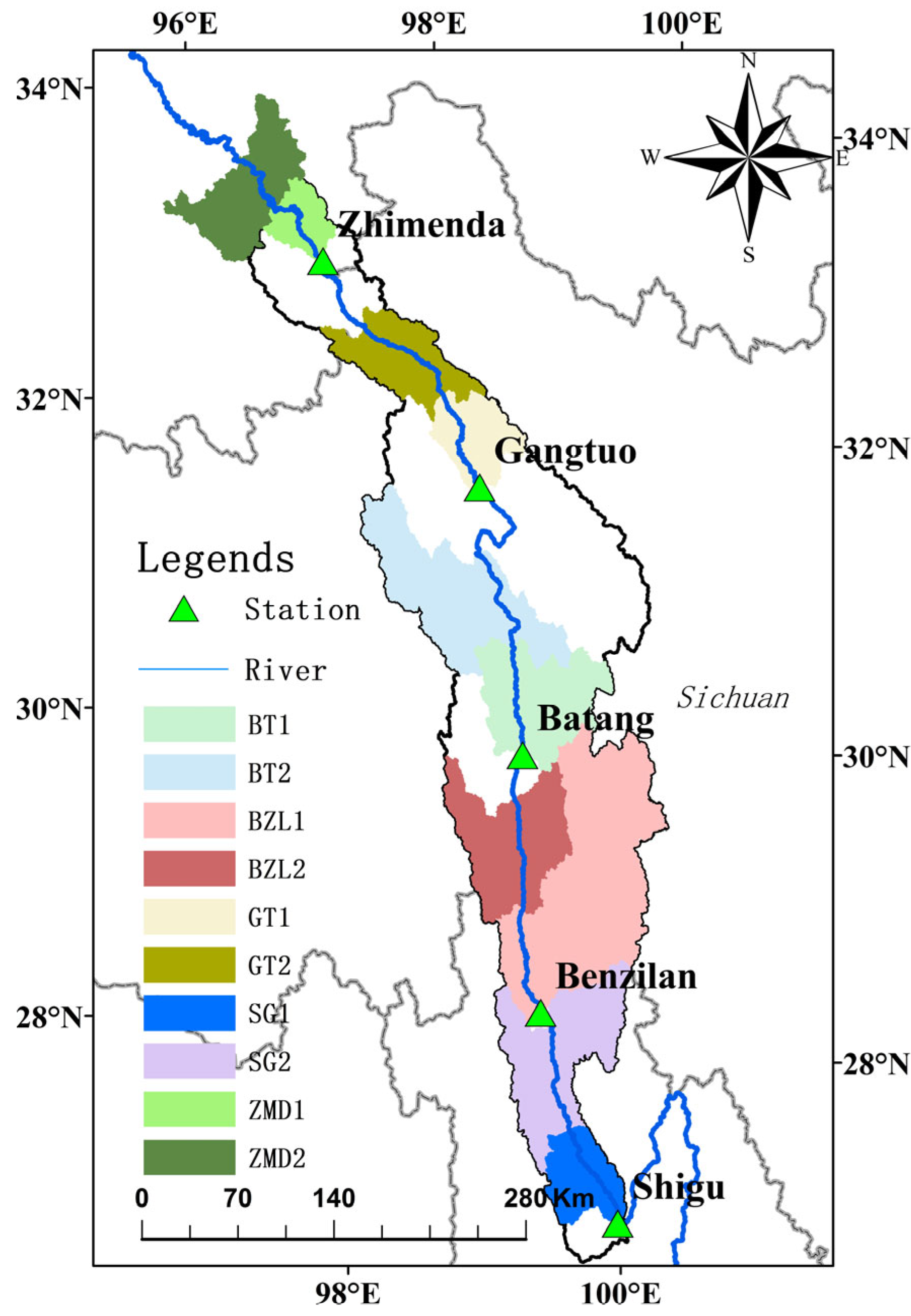
The geographic coordinates of the upper reaches of the Jinsha River range from 97°40′ E to 99°97′ E and from 26°87′ N to 32°64′ N (Figure 1). The section from Batang River Mouth in Yushu County, Qinghai, to the Shigu River in Yulong Naxi Autonomous County, Yunnan, spans approximately 965 km. The upper reaches of the Jinsha River flow through four provinces: Qinghai, Tibet, Sichuan, and Yunnan, and are located in the Hengduan Mountains region. The primary first-order tributaries include 16 rivers, such as the Batang River, Sequ, Maixu River (also known as Dingqu), Zengqu, and Ouq, among others. The river section has an elevation drop of over 1700 m, with an average slope of 1.78‰. The outlet control station is the Shigu Hydrological Station, which controls a catchment area of approximately 214,200 km2. This area is also an important ethnic minority settlement.
During the study period (1980–2021), significant land use changes occurred in the region. Under the combined impacts of climate change and human activities, urban and agricultural land areas increased, while forest and grassland coverage declined. These changes intensified soil erosion and caused fluctuations in ecosystem service values. For example, between 2010 and 2015, the overall equivalent value of ecosystem services increased, yet the ecological vulnerability of the region also intensified.
Furthermore, rapid dam construction has taken place in this area, in alignment with China’s 14th Five-Year Plan. Several large hydropower stations, such as the Batang Hydropower Station, have been completed or are under construction in the upper reaches of the Jinsha River. While these projects have improved clean energy development, they have also altered the hydrological regime, resulting in issues such as reservoir inundation, unstable downstream flows, and compression of aquatic habitats. Potential ecological risks include reduced fish spawning grounds and impacts from cold water releases.

2.2. Research Data Source

(1)
Hydrologic Data
Daily discharge observations from five hydrometric stations—Zhimenda (ZMD), Gangtuo (GT), Benzilan (BZL), Batang (BT), and Shigu (SG)—were collected for 1980–2021 from the Hydrological Yearbook of the People’s Republic of China. Data from 1980–2009 were used for training, and 2010–2021 for testing.
(2)
Meteorological and Other Environmental Element Data
The meteorological dataset consists of the CMA-RA product provided by the China Meteorological Administration, covering the entire drainage basin (i.e., the total contributing catchment; see Section 3.2 Method). It includes daily records of five meteorological variables—precipitation, air temperature, sunshine duration, wind speed, and relative humidity—spanning the period 1980–2021.
(3)
Topographic Data
Topography was represented by the Copernicus DEM (30 m), obtained from the Geospatial Data Cloud (https://www.gscloud.cn). The DEM was primarily used to derive the river network and to delineate the contributing catchments for each cross-section.

3. Methodology

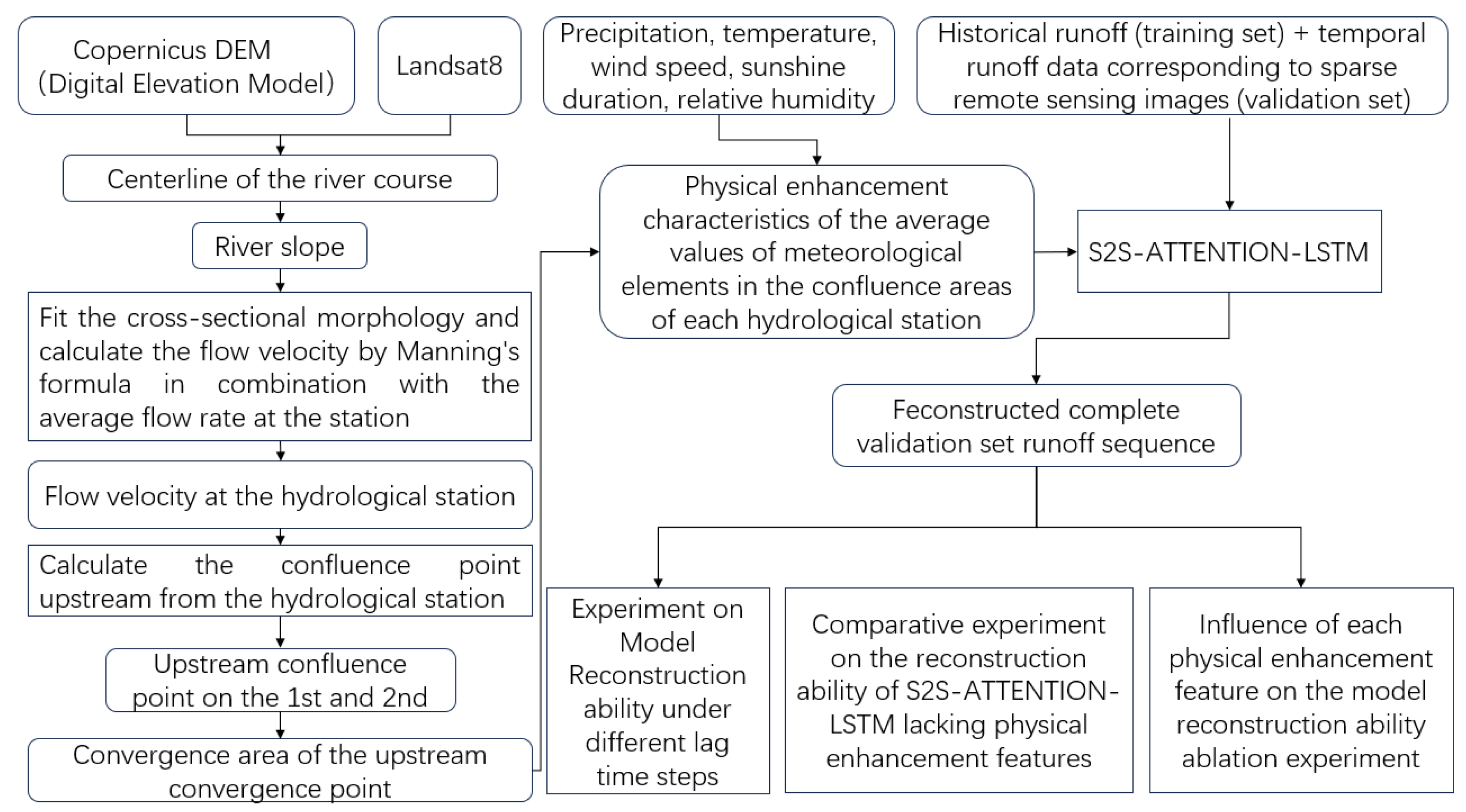
This study proposes a runoff time series reconstruction method that integrates physics-enhanced features with a deep learning model. The technical framework is illustrated in Figure 2. The proposed PSAL model combines a physics-enhanced component (PF) with a Seq2Seq-Attention-LSTM architecture. The physics-enhanced features are derived based on the Isochrone Method [29], while the machine learning component employs a Seq2Seq-Attention-LSTM for streamflow reconstruction [28]. Using the Copernicus DEM and Landsat-8 imagery, we extract the river network for the study area and, together with observed discharge, estimate reach-averaged flow velocity via Manning’s equation. Based on the estimated velocity and the model time step, we infer the daily water travel distance to locate upstream confluence points. We then merge the upstream contributing areas and compute spatial means of daily meteorological variables (precipitation, air temperature, wind speed, sunshine duration, and relative humidity) over these areas as physics-enhanced inputs to the deep learning model.
Next, a Seq2Seq-Attention-LSTM is employed to reconstruct the streamflow series. Historical discharge serves as input, jointly with the spatially averaged meteorological variables and other physical features, for training. To assess effectiveness, we design three experiments: (i) testing the differences in streamflow reconstruction capability under different lag time steps; (ii) comparing against a model without physics-enhanced inputs to quantify the benefit of PF; and (iii) conducting ablation by removing individual physics-enhanced features to evaluate their contributions. This setup elucidates performance under different configurations and informs practical deployment.
The proposed PSAL model integrates physical mechanisms with the strengths of deep learning. Its core idea is to inject key hydrological process information through physics enhancement into both the model structure and input features, thereby improving interpretability, generalization, and spatiotemporal consistency while accomplishing streamflow reconstruction. The PSAL model architecture comprises four main components: physics enhancement, an attention mechanism, an encoder and a decoder, along with an integrated S2S framework. Each component is designed to reinforce the accuracy and stability of streamflow sequence prediction. Section 3.1 introduces the study method, Section 3.2 presents the model principles, and Section 3.3 details the model architecture.

3.1. Principles of the Model

The PSAL model incorporates physics-enhanced features inspired by the equal flow time line method. First, a digital watershed is constructed based on topographic data and subdivided into iso-time contributing areas, following the principles of distributed hydrological modeling. These areas serve as the basic input units for the model. For each day, the corresponding contributing area is identified, and spatially averaged meteorological features within the area are extracted. The Seq-to-Seq Attention LSTM model then simulates streamflow accumulation using its long short-term memory mechanism, while the attention mechanism highlights the physics-enhanced features, enabling efficient and stable reconstruction of daily streamflow series.
By mimicking the physical runoff routing process, the PSAL model introduces a physics-enhanced approach that captures daily contributing areas and their spatial meteorological characteristics. This data structure reflects hillslope runoff generation dynamics, serving as a physically meaningful driver for streamflow modeling.
Traditionally, physics-based hydrology partitions the study area using a DEM into subbasins and elevation-band (HRU) units, thereby defining each unit’s runoff source location and routing path. This spatially explicit discretization allows the model to simulate each unit’s runoff–routing response at different time steps and, via river-network connectivity, to represent basin-scale coupling of runoff generation and routing across time scales. Such structural partitioning is central to capturing the spatiotemporal heterogeneity of watershed hydrologic responses in physical models.
The contributing area construction method proposed in this study, based on DEM and average flow velocity, is conceptually similar to the equal flow time line method [29], and physically approximates the runoff generation and routing response of sub-watershed units. By estimating upstream paths reachable within a day, we effectively identify hydraulically reachable “dynamic subbasin units” under different forecast lead times, and use the synthesized contributing zone to represent the future time-step runoff contribution area to a given cross-section. In other words, this time–space integrated approach approximates the physical sequence of “runoff generated in subbasin units, routed along the river network, and converging at the section,” thereby supplying the deep model with physically grounded input features [30].
This construction has the following hydrological significance: spatially, the routing-influence zone can be viewed as the superposition of responses from multiple subbasin units across time steps; temporally, water travel paths and velocities control the delay of the runoff–routing response; process-wise, spatial means of meteorological variables over the contributing zone act as a weighted integration of the runoff-driving factors across units. Thus, without relying on a full physical model, the proposed contributing-zone meteorological averaging provides a data-structural approximation to subbasin partitioning and response mechanisms, preserving the spatiotemporal coupling of hydrologic processes and supplying deeper physical meaning to the drivers used by the learning model.

3.2. Method

Research methodology: This study uses daily streamflow data from five hydrological stations in the upper Jinsha River for 1980–2021. We construct a dataset that provides the previous 7 days of discharge together with discharge values on dates corresponding to Landsat, Sentinel, and Gaofen satellite overpasses, thereby simulating a streamflow series with missing values. The proposed PSAL model is trained on the training set and then used to infill the test-set streamflow series. We evaluate and analyze results on both the training and test sets. To improve interpolation accuracy, Section 4.2 investigates the optimal time lag by testing different lag steps (T-1 to T-7) across stations and identifying the best lag length per site. We further examine the impact of physics-enhanced features on reconstruction performance via: (i) a baseline experiment using an S2S-Attention-LSTM without any physical features to quantify the contribution of physics enhancement, and (ii) ablation experiments that remove individual physics-enhanced features to assess the model’s sensitivity to each variable.
In addition to streamflow data, input feature matrices are constructed for both the training and testing datasets. Each feature matrix consists of the spatially averaged meteorological variables within the contributing areas on the current day and one day prior. The lead time is set to two days, as a three-day lead would extend the contributing area beyond the upstream gauging station, introducing significant error due to reliance on downstream flow velocities. The included meteorological variables are precipitation, air temperature, wind speed, sunshine duration, and relative humidity. The method for calculating the contributing area is detailed in Section 3.3.1 (Physics Enhancement), and the resulting one-day and two-day contributing areas are shown in Figure 3.
The input and output time lengths of the model are shown in Table 1. A five-fold cross-validation strategy was adopted during model training to ensure robust evaluation [31]. The dataset was randomly divided into five equal subsets (folds), with each fold used once as the validation set and the remaining four used for training. This process was repeated five times to ensure that each fold served as the validation set exactly once, effectively reducing the randomness introduced by data splitting and improving the stability and reliability of model evaluation.
The overall dataset was split based on the time series: data from 1980 to 2009 were used for training, and data from 2010 to 2021 for testing. To enhance the generalization ability of the model, an early stopping strategy was employed—training was halted when the model’s performance on the validation set ceased to improve over consecutive epochs. Additionally, the parameters are optimized by using the commonly used Adam optimizer through the MSE. This optimizer adaptively adjusts the learning rates for individual parameters by computing the exponential moving averages of the first and second moments of the gradients, incorporating momentum to accelerate convergence and improve stability.
The loss function used was Mean Squared Error (MSE), and model parameters were updated by minimizing this loss. To prevent overfitting, learning rate decay was implemented, allowing the learning rate to be dynamically adjusted during training.

3.3. Model Structure

The PSAL model consists of two components: a physics-enhanced module and a Seq2Seq-Attention-LSTM model. The physics-enhanced part calculates meteorological feature values within the contributing areas at different time steps for each station using the equal flow time line method. These features, combined with streamflow sequences, form the input feature matrix, as described in Section 3.3.1. The Seq2Seq-Attention-LSTM component extends the standard Seq2Seq-LSTM by incorporating both temporal and feature-level attention mechanisms. It is responsible for adaptively processing streamflow sequences and other physical features from the input matrix, as detailed in Section 3.3.2.

3.3.1. Physics-Enhanced

Physics-enhanced feature methods, which fuse physical information with data-driven models, show broad application prospects in hydrology. By introducing physical predictors such as precipitation and air temperature, they enhance a model’s ability to capture hydrologic processes, with notable performance in streamflow forecasting, flood early warning, and water resources management. These methods strengthen process representation: by incorporating key physical factors (e.g., precipitation, temperature), physics-enhanced approaches remedy deficiencies of purely data-driven models in representing physical mechanisms, improving predictive accuracy and generalization in data-scarce settings [32], and boosting adaptability in complex environments—especially for flood warning and soil moisture modeling—where they demonstrate high stability [33]. They also improve predictive accuracy and interpretability, providing scientific support for flood mitigation and water resources operations.
The construction of physics-enhanced features in this study involves the following steps: First, river networks are extracted from remote sensing imagery and DEM data, and a series of cross-sections perpendicular to the river channels are generated based on CAD engineering drawings [34]. Elevation profiles are derived from DEM data to calculate slopes and combined with observed discharge data to fit cross-sectional shapes. The Manning equation is then used to estimate average flow velocity along each river segment [35]. Based on this velocity and the time step of simulation, the upstream water propagation distance for each day is calculated. Using river network topology and gauging station locations, daily upstream contributing points are determined [36]. DEM data and the D8 algorithm are applied to identify flow directions of each cell, delineate flow paths and watershed boundaries, and compute the contributing area for each point [37]. Contributing areas within the upstream limit (not exceeding the next upstream gauging station) are merged to form the final daily contributing area. Daily meteorological variables within this area are then extracted and spatially averaged as model input features. This method mimics grid-based units and flow routing mechanisms in physical hydrological models, while retaining the advantages of data-driven modeling, thereby improving the hydrological relevance, spatial responsiveness, and temporal consistency of model inputs—providing more process-representative driving factors for streamflow reconstruction.

3.3.2. S2S-Attention-LSTM

The Seq2Seq-Attention-LSTM model consists of four main components: a physics-enhanced module, an attention mechanism, an encoder, a decoder, and an integrated Seq2Seq framework. Originating from sequence-to-sequence (Seq2Seq) models initially designed for machine translation tasks [38], this architecture has been widely adapted for time series prediction, including hydrological modeling, to capture complex nonlinear dynamics [39,40,41]. The model’s core lies in the encoder–decoder structure: the encoder, built with multi-layer LSTM networks, compresses the input sequence—comprising historical streamflow, meteorological, and physical features—into a fixed-length context vector (hidden state), capturing long-term dependencies and dynamic patterns. The decoder, also based on a multi-layer LSTM, generates the output sequence (i.e., future runoff reconstruction values) step by step, starting from the context vector. During training, the teacher forcing strategy is applied, in which the actual runoff value at the previous time step is fed into the decoder instead of the predicted value. This technique accelerates convergence and improves model stability, enabling more effective reconstruction from past observations to future sequences. LSTM units are central to both encoder and decoder, effectively handling long-term dependencies, seasonal variations, and extreme events by mitigating the vanishing gradient problem. The attention mechanism dynamically assigns weights to emphasize the most relevant parts of the input sequence at each decoding step, improving sensitivity to key hydrological features [42,43]. By integrating physics-enhanced features (e.g., meteorological and soil data), this hybrid model improves spatial generalization and nonlinear response handling, offering enhanced accuracy and robustness in streamflow sequence reconstruction tasks [44,45,46].
The PSAL model used in this paper incorporates an automatic skip mechanism for null values during training, which can adapt to data gaps in the runoff sequence and learn the characteristics of the existing data sequence. At the same time, the model’s hyperparameters were set according to the Seq2Seq-Attention-LSTM situation in (Stefenon et al. (2023) [47]), the best runoff reconstruction effect obtained through multiple debugging, and the final hyperparameters are shown in Table 2. Regarding the model’s objective, Stefenon et al. (2023) [47] focused on short-term water level prediction, with higher data frequencies (such as sensor observations at 5-min intervals), so they set a relatively large number of iterations (100 times) and a higher learning rate (0.001) to accelerate convergence and maintain a faster training efficiency on high-frequency data. This study, however, is focused on daily-scale runoff reconstruction, with smaller data volumes and higher noise, so a lower learning rate (0.0005) was adopted to avoid the model quickly falling into a local optimum in small sample and high fluctuation situations. At the same time, the number of iterations was significantly reduced (10 times), and combined with cross-validation and early stopping mechanisms, it can effectively avoid overfitting and reduce computational costs under limited data conditions. Additionally, this study introduced a medium-sized batch size (batch size = 32) to achieve a balance between model training stability and efficiency.

3.4. Evaluation Index

To comprehensively evaluate the simulation performance of the model, six statistical metrics were employed in this study: the Nash–Sutcliffe Efficiency (NSE), the coefficient of determination (R2), the Normalized Root Mean Square Error (NRMSE), the Relative Mean Absolute Error (RelMAE), the Root Mean Square Error (RMSE), and the Mean Absolute Error (MAE). Among them, NSE, R2, NRMSE, and RelMAE were used to assess model performance under conditions where the lengths of the training and validation datasets differ. In the subsequent analysis of factors influencing the model’s reconstruction ability, the more commonly used metrics—NSE, R2, RMSE, and MAE—were adopted. Its mathematical expression is as follows:
N S E = 1 i = 1 N ( o b s i s i m i ) 2 i = 1 N ( o b s i o b ¯ s ) 2
N R M S E = 1 N i = 1 N ( s i m i o b s i ) 2 o b s m a x o b ¯ s m i n
R e l M A E = i = 1 N s i m i o b s i o b ¯ s N
R 2 = ( i = 1 N ( o b s i o b ¯ s ) ( s i m i s i ¯ m ) ) 2 i = 1 N ( o b s i o b ¯ s ) 2 i = 1 N ( s i m i s i ¯ m ) 2
R M S E = i = 1 N ( s i m i o b s i ) 2 N
M A E = i = 1 N s i m i o b s i N
where simi denotes the model-simulated value, o b s i the observed value, o b ¯ s the mean of observations, s i ¯ m the mean of simulations, and N the total number of observations. Among these four statistical indices, NSE (Nash–Sutcliffe efficiency) is one of the most commonly used metrics in hydrologic modeling to assess the goodness of fit between simulations and observations. The closer NSE is to 1, the stronger the fit; NSE > 0.5 indicates good performance, and NSE > 0.8 indicates excellent performance; R2 (coefficient of determination) evaluates the correlation between simulated and observed values, ranging from 0 to 1. Values closer to 1 imply better fit, but note that R2 does not fully capture model bias. NRMSE is a dimensionless form of RMSE, typically normalized by the range of observed values (i.e., the difference between the maximum and minimum observations). It measures the proportion of model error relative to the overall variability of the data. A lower NRMSE indicates that the simulated values are closer to the observations, and it facilitates performance comparison across different stations or time periods. However, since it is based on squared errors, NRMSE is also sensitive to outliers; RelMAE is a normalized form of MAE, in which the mean absolute error is scaled by the mean of the observed values. It expresses the model error as a proportion of the typical magnitude of the observations. RelMAE provides an intuitive measure of relative error, with smaller values indicating higher relative accuracy of the model. RMSE (root mean square error) is the square root of the mean squared difference between simulations and observations; smaller values indicate simulations are closer to observations. Because it squares errors, RMSE is sensitive to outliers; MAE (mean absolute error) computes the mean absolute difference between simulations and observations, providing a more balanced view of errors; smaller MAE indicates lower overall error.
To comprehensively evaluate the model’s performance across different flow regimes—particularly its ability to identify high and extreme flow events—this study introduces a threshold-based classification approach as a supplementary assessment. The observed streamflow data were first divided into quantiles based on their distribution, with the 80th percentile (P80) and 90th percentile (P90) used as thresholds for high-flow and extreme high-flow events, respectively. Specifically, a day with observed streamflow ≥ P80 is defined as a high-flow event, and ≥P90 as an extreme high-flow event. The reconstructed streamflow was then classified using the same thresholds and compared with the observed classifications to construct a confusion matrix. Based on this, classification performance metrics were calculated, including Accuracy (the proportion of correctly classified cases), Precision (the proportion of predicted high-flow events that are correct), Recall (the proportion of actual high-flow events correctly identified), and F1 Score (the harmonic mean of precision and recall, reflecting the balance between accuracy and completeness in high-flow event detection). The mathematical definitions of these metrics are as follows:
Accuracy = T P + T N T P + T N + F P + F N
Precision = T P T P + F P
Recall = T P T P + F N
F 1   Score = 2 × Precision × Recall Precision + Recall
Here, TP (True Positive) represents the number of high-flow events correctly identified by the model, FP (False Positive) refers to non-high-flow events incorrectly classified as high-flow, FN (False Negative) denotes high-flow events that the model failed to detect, and TN (True Negative) refers to correctly identified non-high-flow events. This method helps quantitatively assess the model’s capability in detecting extreme events, revealing prediction blind spots that regression metrics may overlook, and thereby provides more targeted insights for model improvement and practical evaluation.

4. Results and Evaluation

4.1. Data and Model Feature Analysis

In the study of runoff reconstruction, the completeness of the data, the characteristics of its spatial and temporal distribution, and the setting of the model’s hyperparameters all directly affect the training effect and simulation ability of the model. This section explains the data characteristics and the setting of the model’s hyperparameters.
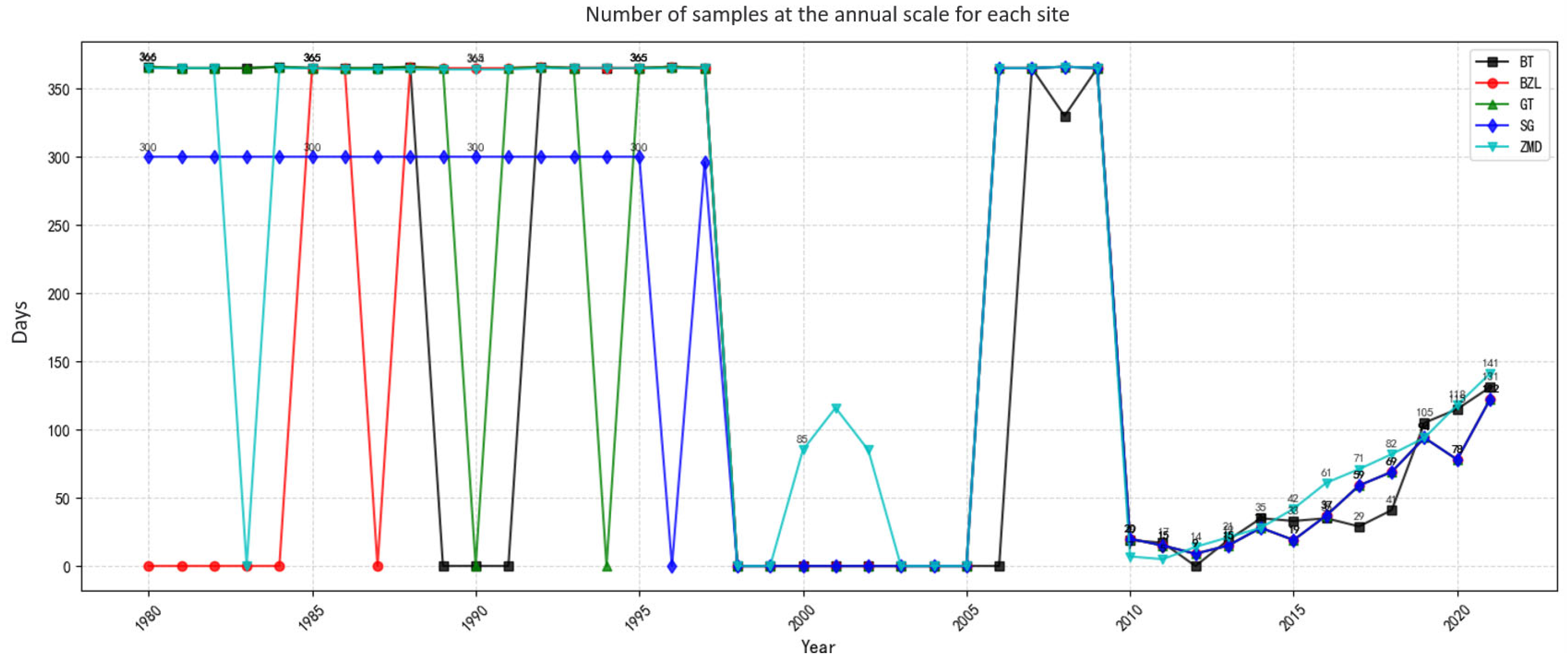
From the annual data distribution (Figure 4), it can be seen that the flow data of the runoff dataset used for training and testing showed significant phased changes during the period from 1980 to 2021. Due to the data gap in the hydrological yearbook, there were almost no data from all monitoring stations from 1996 to 2005. In the late 20th century, from 1980 to 1995, most hydrological stations had relatively complete runoff data, with only some years having missing data. The most severe case was BZL (with data missing for 6 years). From 2005 to 2009, the runoff data of almost all hydrological stations was relatively complete (except for BT in 2006). From 2010 to 2021, it was classified as the test set, and the number of runoff data was the same as the number of corresponding dates of remote sensing data. After 2015, the annual data volume at each station increased significantly. The annual average exceeded 50 times, and after 2020, it even reached more than 80 times. For example, the data volume of BT Station in 2015 was 31 days, while it increased to 97 days in 2021. The stations of BZL, GT, SG, and ZMD also showed similar growth trends. This trend is closely related to the development of remote sensing technology and the increase in high-resolution satellite data, which significantly increased the data density and provided more abundant samples for machine learning modeling.

4.2. Evaluation of Model Simulation Results

The prediction results of the fully factor-driven model are presented in Table 3, indicating that the model exhibits generally good fitting performance across all cross-sections. Overall, the model performs excellently on the training dataset, with NSE values exceeding 0.90 at all five stations and an average NSE reaching 0.95. The average coefficient of determination (R2) is 0.98, suggesting that the model effectively captures the hydrological response characteristics of each basin. Among them, the SG and BZL sections show the most outstanding performance in the training set, with NSE values of 0.97 and R2 as high as 0.99. The corresponding NRMSE values are 0.0295 and 0.0278, while the RelMAE values are 0.0856 and 0.0893, respectively. These results demonstrate a high degree of agreement between the simulated and observed values, with low error levels and excellent fitting accuracy.
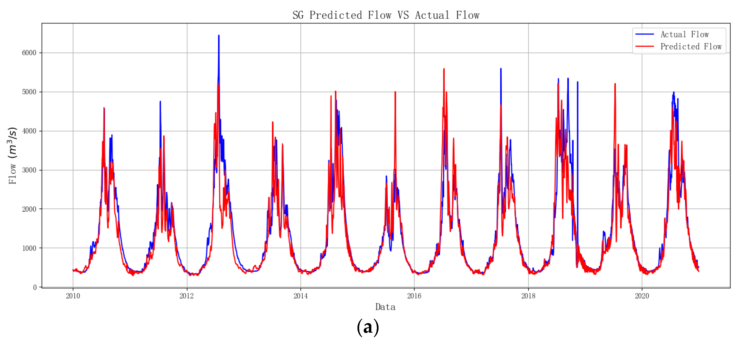
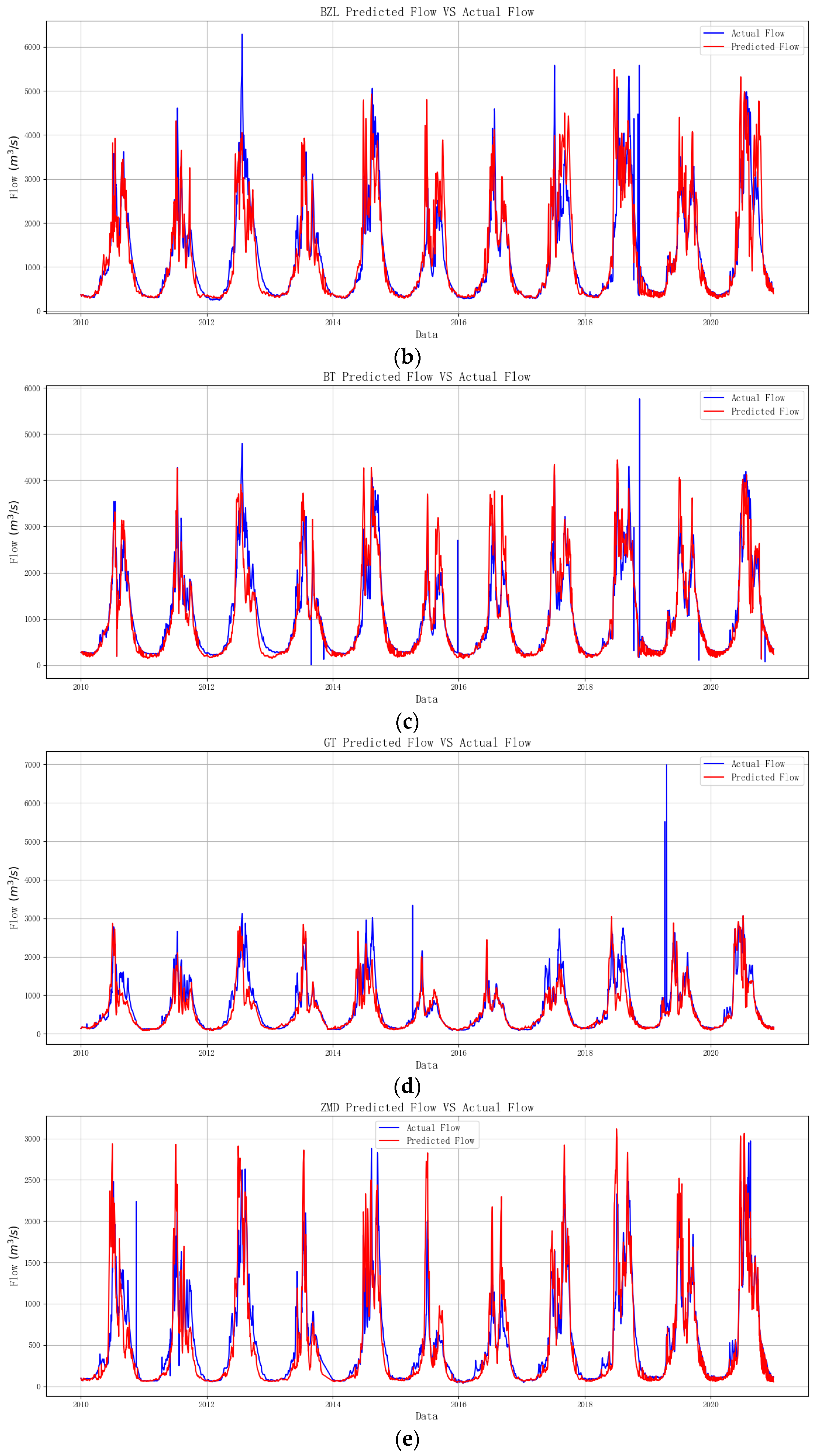
The predictive performance of the PSAL model is summarized in Table 3. The simulation results on the test set are shown in Figure 5a–e. Overall, it shows strong fitting ability across all stations, particularly on the training set, where NSE values exceed 0.90 and average 0.95, with an R2 of 0.98. Notably, the SG and BZL stations achieve the best results in the training phase, both with NSEs of 0.97 and R2 values of 0.99. Their low NRMSE (0.0295 and 0.0278) and RelMAE (0.0856 and 0.0893) indicate high simulation accuracy and close agreement with observations.
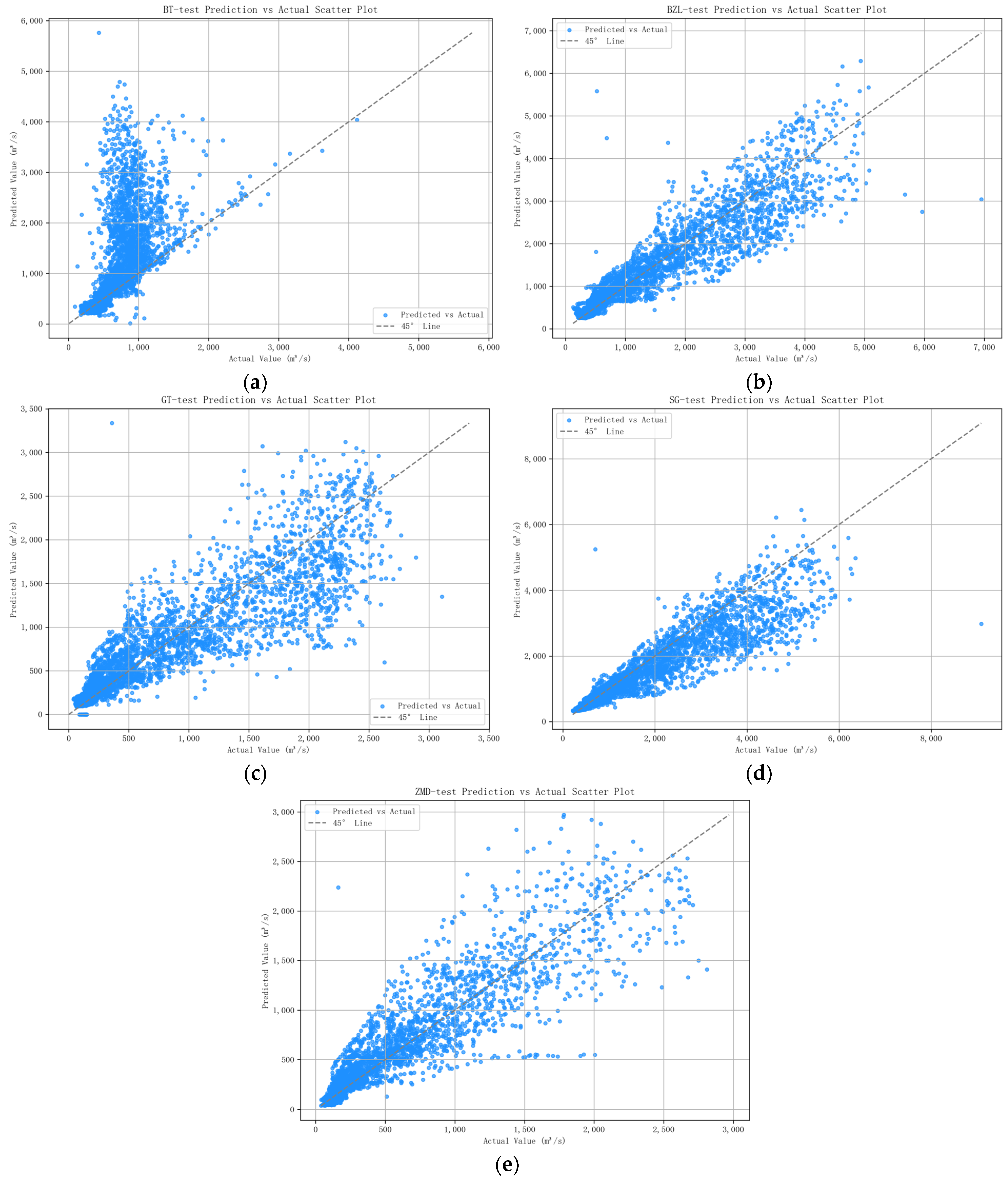
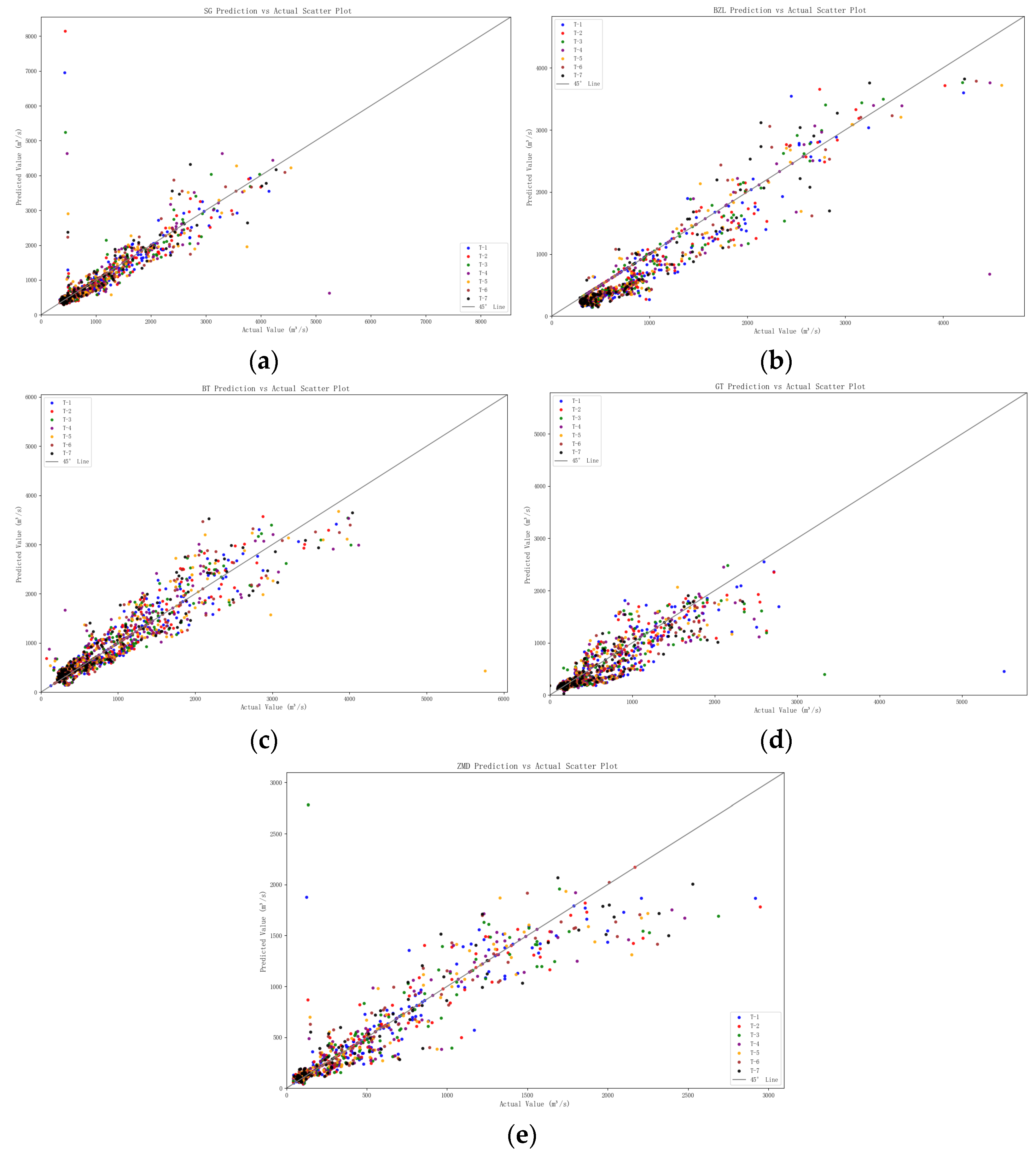
On the test set, the model maintains good generalization ability. The average NSE across all stations is 0.81 and R2 is 0.91, reflecting reliable performance on unseen data. However, the BT station, despite achieving a relatively high NSE of 0.89 and R2 of 0.94, shows clear signs of overestimation at low flow levels, as seen in Figure 6a. This pattern leads to a noticeable deviation from the 1:1 line in the scatter plot, indicating systematic bias. Additionally, the station exhibits relatively large error metrics (NRMSE = 0.21, RelMAE = 0.72), suggesting that the model’s predictive accuracy at BT is limited. Overall, aside from the BT station, the scatter plots of other stations show a relatively uniform distribution of errors across the full range of flow values.
In contrast, the performance at the GT station is relatively lower in the test set, with an NSE of 0.71, R2 of 0.85, NRMSE of 0.13, and RelMAE of 0.28. While the general trend is still captured, the simulation accuracy declines. This may be attributed to the influence of nonlinear factors such as frequent rainfall and snowmelt processes, which increase the model’s difficulty in handling sudden high-frequency runoff fluctuations [30]. Moreover, the SG station shows a decline in test performance compared to the training set, with an NSE of 0.80, R2 of 0.92, NRMSE of 0.07, and RelMAE of 0.20. Although the error remains within an acceptable range, the reduction in accuracy may be related to the complex terrain and enhanced instability in runoff pathways at this section [29].
In conclusion, the PSAL model demonstrates excellent simulation capabilities in the reconstruction of runoff sequences (Figure 5). The performance differences among stations can be attributed to the complexity of local hydrology. For instance, the BZL and ZMD stations benefit from relatively stable flow patterns, which the model can capture more easily. In contrast, stations like GT exhibit greater variability, leading to increased prediction errors. Additionally, some stations such as BT, while demonstrating generally good simulation performance, still show noticeable prediction errors at certain flow levels—particularly during low-flow conditions.
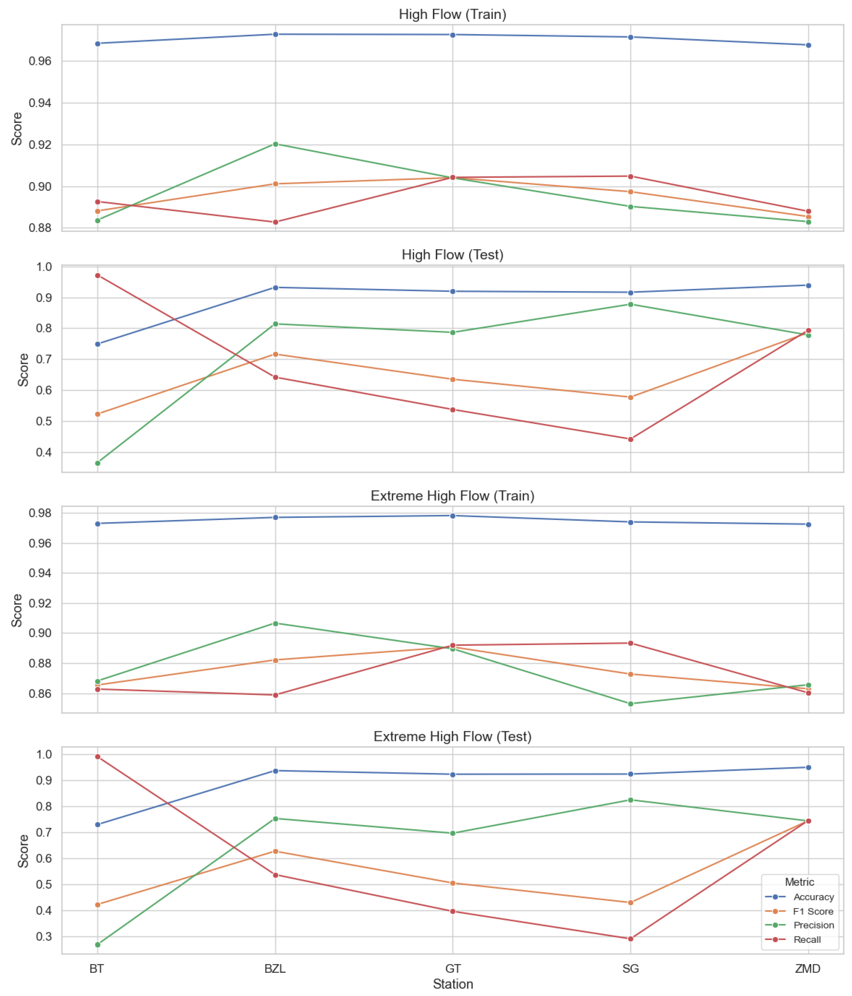
To evaluate the model’s accuracy in simulating high and extreme flow events, this section analyzes four performance metrics—Accuracy, F1 Score, Precision, and Recall—based on 80% and 90% streamflow thresholds across all stations for both training and testing sets. The results are shown in Figure 7.
Overall, the model performs well on the training set, with most metrics exceeding 0.9 across all stations. For example, under the “High Flow–Train” condition, the GT station achieved an accuracy of 0.967 and an F1 score of 0.9174, while SG performed even better with an accuracy of 0.9689 and an F1 score of 0.922, indicating that the model effectively learned the key features of high-flow events during training.
On the testing set, although performance slightly declined, the model still maintained strong generalization. For instance, GT and ZMD remained stable under the “High Flow–Test” scenario, with F1 scores of 0.7661 and 0.8283, respectively. In contrast, BT showed a lower F1 score of 0.6239 and a precision of 0.4633, but had a high recall of 0.9549, suggesting a tendency toward over-detection—likely related to high streamflow variability at that station.
Under extreme high-flow conditions, prediction difficulty increased, especially in the testing phase, with some stations showing notable drops in performance. For example, in the “Extreme High Flow–Test” scenario, SG’s F1 score dropped to 0.4301, with a high precision of 0.8239 but a low recall of 0.291, indicating limited detection capability for extreme events. In contrast, ZMD remained the most stable, achieving an F1 score of 0.744 and an accuracy of 0.9487 even under extreme conditions, highlighting its consistent data structure and the model’s adaptability.
In summary, ZMD and GT stations demonstrated the most stable and reliable performance, making them suitable for further extreme event prediction. While BT and SG showed greater variability—particularly in precision and recall on the test set—the model still maintained a generally high level of accuracy in simulating high-flow events across stations.

4.3. The Influence of Lag Time Step Size on Refactoring Capability

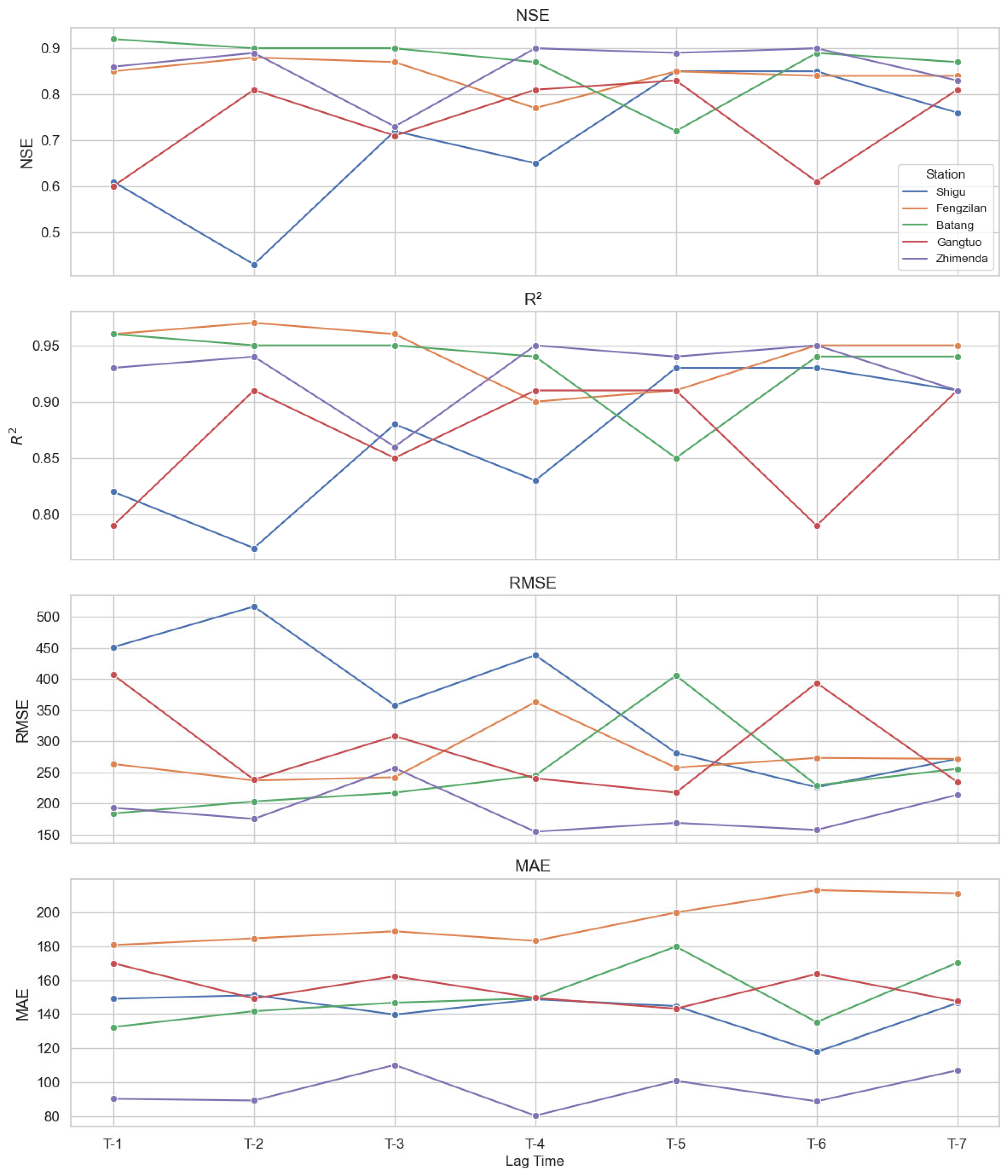
To explore the optimal lag time step for the operation of the PSAL runoff reconstruction model, error analysis of the model reconstruction results under lag time steps of T-1 to T-7 days was conducted in this section.
As shown in Figure 8, the line chart of reconstruction errors under lag times T-1 to T-7 for each station indicates that the PSAL model exhibits significant differences in fitting accuracy and variability across different lag periods. Overall, at T-7, most stations achieve better fit (NSE = 0.84), yet inter-station dispersion remains pronounced. Figure 9 is the runoff reconstruction simulation—measured scatter plot of SG, BZL, BT, GT and ZMD stations under different lag times. As lag changes, reconstructed points at some stations progressively deviate from the 45° reference line—especially in the high-flow range—indicating reduced responsiveness to extremes under certain lag conditions. For example, at SG, the scatter dispersion increases markedly at T-2 and T-4, with reconstructions drifting farther from observations, whereas at T-6, the fit improves substantially, with a tighter point cloud closer to the 45° line, suggesting stronger process fidelity at longer lags. In contrast, BT shows concentrated, well-fitted points at T-1, but performance degrades with increasing lag, and by T-5 the fit diverges noticeably, implying sensitivity of its hydrologic response to temporal delay. ZMD performs best at T-4, with reconstructed values densely clustered near the 45° line, while larger deviations appear at T-3 and T-7, reflecting volatility at medium-to-long lags. At GT, the T-6 reconstruction is more concentrated and closer to the ideal fit line than at T-1, indicating the model maintains strong stability under longer lag conditions.
Overall, the scatterplot results are consistent with the tabulated metrics. At each station’s optimal lag step, PSAL attains NSE values above 0.83, indicating robust overall reconstruction capability. While T-7 performs well at most stations, it is not universally optimal. Some stations maintain strong reconstruction accuracy at longer lags, such as T-3 or T-6, implying that the optimal lag differs under varying hydrologic conditions, with these differences becoming more pronounced in high-flow situations.

4.4. Ablation Experiment: Results and Analysis

Meteorological factors not only provide precipitation forcing but also strongly regulate energy budgets and water transformation pathways during runoff generation, jointly determining whether precipitation becomes effective runoff. By participating in surface energy balance processes, these factors indirectly modulate the efficiency of precipitation-to-runoff conversion and shape the spatiotemporal characteristics of runoff generation. After precipitation reaches the land surface, it undergoes canopy interception, surface storage, soil infiltration, and interflow, among other stages. Throughout this process, other meteorological variables play key regulatory roles: air temperature affects evapotranspiration rates and soil freezing conditions—higher temperatures enhance evaporation and reduce effective runoff, while in snow-dominated areas they control the timing of meltwater release; humidity reflects atmospheric saturation and influences vapor transport capacity—higher humidity lowers evaporative demand and favors water retention; wind speed alters air–water exchange rates and evaporation intensity, with pronounced evapotranspiration losses under dry, windy conditions; sunshine duration, as a direct indicator of surface energy input, governs potential evaporation and strongly affects latent and sensible heat fluxes, thereby determining phase changes (liquid–vapor) and soil moisture status. Incorporating these variables into the inputs enables a more comprehensive depiction of the hydrologic system’s physical state and strengthens the model’s ability to represent nonlinear processes.
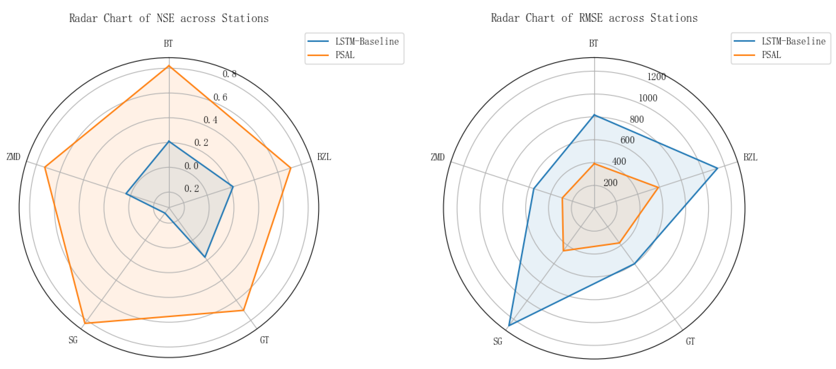
To evaluate the impact of physics enhancement on PSAL’s reconstruction ability, we construct a baseline model—an S2S-Attention-LSTM without physical enhancement (LSTM-Baseline). Relative to PSAL, the LSTM-Baseline removes only the daily meteorological physical-feature inputs while retaining the attention mechanism. The dataset split and reconstruction experiments are kept identical to those of PSAL.
The S2S-Attention-LSTM streamflow reconstruction model without daily physical features performs poorly overall on long time-series simulations (Table 4). NSE values are generally below 0.3, and some stations even show negative values (e.g., SG, NSE = −0.27), indicating a poor fit to the runoff response in these areas. Among stations, BZL performs relatively better (NSE = 0.22, R2 = 0.57). This contrasts markedly with PSAL: stations that perform well under PSAL exhibit weak simulation capability in the LSTM-Baseline. This discrepancy is likely tied to complex topographic controls and strong meteorological influences, causing the two models to behave differently at the same sites. In particular, SG is situated in a high-mountain gorge where rainfall–runoff responses are strongly affected by terrain, soil structure, and routing pathways; relying solely on sequence data, the LSTM-Baseline struggles to effectively simulate long-term runoff in the absence of auxiliary physical features.
By comparison, the proposed PSAL model exhibits clear advantages at all stations (Figure 10). By incorporating key daily physical factors (e.g., precipitation and air temperature), it substantially improves characterization of the rainfall–runoff process. Across the five stations, NSE exceeds 0.81, R2 is above 0.85, and both RMSE and MAE are markedly lower than those of the other two models. For example, at BT, PSAL raises NSE to 0.89 and reduces RMSE to 308, delivering a large error reduction relative to baseline model and highlighting the importance of physical features for capturing complex routing and lagged responses.
To further assess the impact of individual meteorological factors, we conduct ablation experiments that sequentially remove the contributing-area meteorological inputs for the current day (denoted “1” in the table) and for a 1-day lead (denoted “2”), and evaluate how performance changes under different input combinations. The results are shown in Table 5.
Figure 11 presents the heatmaps of ablation experiment results at the five stations. The results show that, except for the BT station, where removing any meteorological variable leads to a substantial decline in performance, the impacts of excluding individual meteorological features are relatively minor at the other stations. This indicates that the model’s reconstruction capability arises from the combined effect of multiple meteorological drivers. Precipitation, as the primary driver of runoff generation, exerts a particularly significant influence on model performance. Across all stations, removing the precipitation variable consistently reduced model performance (ΔNSE = −0.32). At the BT station, removing ‘Precipitation 1’ reduced the NSE to 0.15 and increased the RMSE to 846.40, rendering the model nearly ineffective, thereby underscoring the decisive role of precipitation in streamflow reconstruction.
Similar patterns appear elsewhere: at ZMD, removing Precipitation_1 lowers NSE to 0.76 and raises RMSE to 277.80; at GT, removing Precipitation_2 lowers NSE to 0.51 with RMSE up to 480.43; at SG, removing Precipitation_2 lowers NSE to 0.46 with RMSE up to 832.55. These results further confirm the stable, key physical significance of precipitation across regions.
Beyond precipitation, sunshine and humidity also exert notable—yet spatially heterogeneous—impacts. At BT, removing Sunshine_2 or Humidity_2 causes sharp degradation (NSE to −0.09 and −0.07; RMSE to 959.14 and 951.91), suggesting discharge there is strongly driven by complex energy processes, with sunshine and humidity closely tied to evaporation and snowmelt. At BT, removing Humidity_1 and Humidity_2 also markedly reduces NSE (to 0.14 and −0.07), weakening predictive ability. At BZL, sensitivity to wind speed and temperature is higher: removing Wind_1 or Temperature_2 raises RMSE to 411.12 and 421.80, implying that under plateau terrain, wind and temperature strongly regulate evapotranspiration and soil infiltration, indirectly affecting runoff efficiency. GT and ZMD show relatively balanced dependencies; performance declines when individual variables are removed, but by smaller margins, indicating more stable hydrologic response mechanisms and stronger model robustness.
Furthermore, the removal of some features even slightly enhanced the model’s performance. For instance, the NSE of the SG station was 0.79 after removing “Sunshine 2”, which was slightly higher than 0.55 after removing “Sunshine 1”. This indicates that there might be collinearity or redundancy in certain meteorological variables.
Overall, the ablation experiments validate both the physical meaning and predictive contribution of each meteorological variable in the inputs. Precipitation is indispensable as the primary driver of runoff generation, while temperature, humidity, wind speed, and sunshine serve as regulatory factors that provide important complementary benefits to model performance. The degree of dependence on each variable varies by station, reflecting spatial heterogeneity in watershed response mechanisms and supporting the physical rationality and adaptability of constructing inputs from contributing-area meteorological averages. This indicates that although runoff formation is jointly driven by multiple meteorological and geographic factors, precipitation is the most direct source of runoff. In the study area, water supply is dominated by effective precipitation—that is, the portion of rainfall remaining after subtracting evapotranspiration and infiltration losses. Although snow/ice melt and groundwater baseflow may also contribute to runoff, precipitation-driven runoff dominates under the land-use and climatic conditions of this region.

5. Discussion

The proposed PSAL model demonstrates notable advantages in reconstructing daily streamflow series, particularly in data-scarce basins with limited discharge observations. By incorporating physics-enhanced inputs and attention mechanisms, experiments across multiple river sections show that the model not only outperforms conventional deep learning approaches overall but also offers improved adaptability in capturing flow variability and responding to extreme events.

5.1. Relationship Between Model Performance and Hydrologic Response Mechanisms

With all features included, the model achieves high predictive accuracy across five representative stations (mean NSE = 0.81, R2 = 0.91), demonstrating strong adaptability to plateau rivers with complex hydrologic response characteristics. The BT station exhibits the most stable performance—particularly at the T-1 lag—where the model achieves a high goodness of fit (NSE = 0.89). This aligns with the stable hydrologic regime and well-defined flow variation patterns in BT’s contributing area.
In contrast, the GT and SG stations show larger simulation errors, with especially degraded performance at shorter lags (T-1). This is likely due to steep topography, complex hydrological responses, and frequent extreme flow events. These findings highlight ongoing challenges for the model in handling highly dynamic and volatile hydrologic processes.

5.2. Importance and Contribution of Physics-Enhanced Inputs

Meteorological inputs in this study are constructed by back-calculating the daily hydraulically reachable contributing area using digital elevation models (DEM), channel velocity, and the river network structure. This approach reflects the dynamic upstream response units at different time steps. Spatial averages of meteorological variables are then computed within these contributing zones. Physically, this approximates the spatial discretization and runoff-routing processes used in traditional hydrologic models (i.e., subbasins and HRUs), effectively capturing key physical characteristics of runoff generation and flow routing. This enhances the model’s interpretability, generalization ability, and spatiotemporal consistency.
Ablation experiments further confirm the contributions of individual variables. As the primary driver of runoff, precipitation plays a decisive role. Its removal leads to significant performance degradation or even collapse (mean ΔNSE ≈ −0.32); for example, at BT, the NSE drops to 0.15 and RMSE increases to 846.40. This clearly indicates that sequence memory alone is insufficient to capture the fundamental transfer relationship between rainfall and runoff.
Other meteorological factors—such as temperature, humidity, wind speed, and sunshine duration—exhibit spatially heterogeneous importance. For instance, at the SG station, removing temperature reduces the NSE to 0.41, suggesting that energy-related processes strongly influence flow variability in this region. These results also imply that synergistic effects among meteorological variables are especially critical in hydrologic modeling for mountainous areas. Overall, the findings reinforce the necessity of incorporating meteorological features, particularly in complex terrain where different physical drivers exert region-specific impacts on runoff generation and routing.

5.3. Comparison with Existing Studies and Innovations

Compared with prior work, this study achieves several innovations: (1) Under sparse remote sensing data conditions, the integration of physics enhancement with LSTM enables an approximate representation of the hydrological runoff generation and routing processes, thereby enhancing the model’s hydrological consistency and interpretability. (2) It integrates meteorology-driven physics enhancement and, through ablation experiments, confirms the critical role of precipitation features in streamflow reconstruction. (3) It conducts systematic empirical evaluations at multiple typical high-mountain gorge sections, verifying broad applicability for daily runoff reconstruction across complex hydrologic settings.
Relative to the pure LSTM structure of Kratzert et al. (2018) [17] or the runoff-simulation framework that fuses remote sensing with neural networks proposed by Xue et al. (2022) [21], our model goes further by combining physical structural information with an attention mechanism. This yields a deep architecture that unites the strengths of process-driven and data-driven approaches, offering a new paradigm for remote-sensing-led streamflow data reconstruction.

5.4. Limitations and Future Research

Despite promising results, the model has several limitations: (1) The model demonstrates a tendency to overestimate low-flow conditions at certain stations and exhibits limited responsiveness to extreme flow events. Particularly at sites with high runoff variability, the reconstruction accuracy of extreme values remains suboptimal. These findings suggest that further refinement of the model’s reconstruction mechanisms is required to improve its performance under diverse hydrological conditions. (2) The model requires training data with adequate temporal coverage, restricting use in regions with severe scarcity of historical observations. (3) No explicit treatment of uncertainty in remote-sensing source data, which may affect stability.
Future work can proceed along: (1) Introducing constraints for extremes or uncertainty modeling to enhance robustness in high-risk scenarios. (2) Incorporating structure-aware models such as graph neural networks (GNNs) to better extract spatial structural information. (3) Exploring joint calibration of remote sensing and in situ observations to improve accuracy and stability in data-scarce regions.

6. Conclusions

Targeting mountainous basins with sparse remote sensing and missing ground observations, this study proposes a physics-enhanced deep learning model (PSAL) for reconstructing sparse daily streamflow series. Building on a conventional S2S-LSTM, the model introduces attention mechanism at both temporal and feature levels and integrates physics-enhanced hydrological mechanisms, thereby improving representation of discharge temporal dynamics and physical consistency.
Empirical findings from five upper Jinsha River stations show:
(1)
The model demonstrated strong overall performance, with an average NSE of 0.81 and R2 of 0.91 on the test set, significantly outperforming the baseline LSTM model without physical features. It also showed good accuracy in capturing extreme flow events, confirming the critical role of the physics-enhanced mechanism in improving prediction accuracy. Precipitation was identified as the most important driving factor, while other meteorological variables—such as temperature, humidity, wind speed, and sunshine duration—showed station-specific impacts on model performance, reflecting the spatial heterogeneity of regional hydrological responses.
(2)
The contributing-area meteorological averaging not only boosts performance but also, in physical terms, approximates the “subbasin delineation + runoff–routing” mechanism of traditional hydrologic models, enabling data-driven modeling to retain high physical consistency and generalization even without a full physical structure.
(3)
Lag-step experiments indicate better performance at the T-7 setting. Differences in the optimal lag across stations reveal complex influences of underlying-surface heterogeneity on runoff generation and travel times.
In sum, PSAL provides an effective pathway for remote-sensing-led daily streamflow reconstruction that combines physical mechanisms with data-driven advantages, particularly suitable for complex terrain and observation-sparse regions. Future research may incorporate uncertainty modeling, GNN-based structures, or physics-constrained regularization to improve responses to extreme hydrologic events and cross-region generalization, thereby offering stronger technical support for digital-twin watersheds and historical hydrologic data infilling.

Author Contributions

Conceptualization, Z.Y. and T.X.; methodology, Z.Y. and H.Y.; software, L.W.; validation, Z.Y., T.X. and H.Y.; formal analysis, H.Y.; investigation, Z.Y., H.Y.; resources, Z.Y. and T.X.; data curation, H.Y.; writing—original draft preparation, H.Y.; writing—review and editing, Z.Y. and H.Y.; visualization, H.Y.; supervision, L.W.; project administration, L.L. and L.W.; funding acquisition, L.L. All authors have read and agreed to the published version of the manuscript.

Funding

This research was funded by China Yangtze Power Co., Ltd., grant number Z432402001.

Data Availability Statement

The data presented in this study are available on request from the corresponding author due to privacy restrictions.

Acknowledgments

We used ChatGPT-4o-Latest (OpenAI) for minor language polishing and grammar checking. All scientific content was written and validated by the authors.

Conflicts of Interest

The authors declare that this study received funding from China Yangtze Power Co., Ltd. The funder had the following involvement with the study: conceptualization, validation, supervision, and project administration. Zhaokai Yin and Lili Liang were employed by the Institute of Science and Technology, China Three Gorges Corporation. Tao Xu and Lin Wang were employed by the Three Gorges Cascade Dispatch and Communication Center, China Yangtze Power Co., Ltd. Huiqiang Ye declares that the research was conducted in the absence of any commercial or financial relationships that could be construed as a potential conflict of interest.

References

  1. Tang, Q.; Gao, H.; Lu, H.; Lettenmaier, D.P. Remote Sensing: Hydrology. Prog. Phys. Geogr. 2009, 33, 490–509. [Google Scholar] [CrossRef]
  2. Al-Yaari, A.; Juszczak, R. Challenges and Limitations of Remote Sensing Applications in Northern Peatlands: Present and Future Prospects. Remote Sens. 2024, 16, 591. [Google Scholar] [CrossRef]
  3. Junqueira, A.M.; Mao, F.; Mendes, T.S.G.; Simões, S.J.C.; Balestieri, J.A.P.; Hannah, D.M. Estimation of River Flow Using CubeSats Remote Sensing. Sci. Total Environ. 2021, 788, 147762. [Google Scholar] [CrossRef]
  4. Lettenmaier, D.P.; Alsdorf, D.; Dozier, J.; Huffman, G.J.; Pan, M.; Wood, E.F. Inroads of Remote Sensing into Hydrologic Science during the WRR Era. Water Resour. Res. 2015, 51, 7309–7342. [Google Scholar] [CrossRef]
  5. Li, D.R. China’s High-Resolution Earth Observation System (CHEOS): Advances and Perspectives. ISPRS Ann. Photogramm. Remote Sens. Spat. Inf. Sci. 2022, 3, 583–590. [Google Scholar] [CrossRef]
  6. Notti, D.; Giordan, D.; Caló, F.; Pepe, A.; Zucca, F.; Galve, J.P. Potential and Limitations of Open Satellite Data for Flood Mapping. Remote Sens. 2018, 10, 1673. [Google Scholar] [CrossRef]
  7. Adıyaman, H.; Varul, Y.E.; Bakırman, T. Stripe Error Correction for Landsat-7 Using Deep Learning. PFG–J. Photogramm. Remote Sens. Geoinf. Sci. 2025, 93, 51–63. [Google Scholar] [CrossRef]
  8. Blagojević, B.; Mihailović, V.; Bogojević, A.; Plavšić, J. Detecting Annual and Seasonal Hydrological Change Using Marginal Distributions of Daily Flows. Water 2023, 15, 2919. [Google Scholar] [CrossRef]
  9. Xie, T.; Zhang, G.; Hou, J.; Xie, J.; Lv, M.; Liu, F. Hybrid Forecasting Model for Non-Stationary Daily Runoff Series: A Case Study in the Han River Basin, China. J. Hydrol. 2019, 577, 123915. [Google Scholar] [CrossRef]
  10. Ri, T.; Jiang, J.; Sivakumar, B.; Pang, T. A Statistical–Distributed Model of Average Annual Runoff for Water Resources Assessment in DPR Korea. Water 2019, 11, 965. [Google Scholar] [CrossRef]
  11. Swagatika, S.; Paula, J.C.; Sahoo, B.B.; Gupta, S.K.; Singh, P.K. Improving the Forecasting Accuracy of Monthly Runoff Time Series of the Brahmani River in India Using a Hybrid Deep Learning Model. J. Water Clim. Change 2024, 15, 139–151. [Google Scholar] [CrossRef]
  12. Cao, Y.; Fu, C.; Yang, M. Integrating Hourly Scale Hydrological Modeling and Remote Sensing Data for Flood Simulation and Hydrological Analysis in a Coastal Watershed. Water 2023, 13, 10409. [Google Scholar] [CrossRef]
  13. Fok, H.S.; Chen, Y.; Zhou, L. Prospects for Reconstructing Daily Runoff from Individual Upstream Remotely-Sensed Climatic Variables. Remote Sens. 2022, 14, 999. [Google Scholar] [CrossRef]
  14. Akoko, G.; Le, T.H.; Gomi, T.; Kato, T. A Review of SWAT Model Application in Africa. Water 2021, 13, 1313. [Google Scholar] [CrossRef]
  15. Ren, Y.; Zeng, S.; Liu, J.; Tang, Z.; Hua, X.; Li, Z.; Song, J.; Xia, J. Mid- to Long-Term Runoff Prediction Based on Deep Learning at Different Time Scales in the Upper Yangtze River Basin. Water 2022, 14, 1692. [Google Scholar] [CrossRef]
  16. Xu, D.-M.; Hu, X.-X.; Wang, W.-C.; Chau, K.-W.; Zang, H.-F.; Wang, J. A New Hybrid Model for Monthly Runoff Prediction Using ELMAN Neural Network Based on Decomposition-Integration Structure with Local Error Correction Method. Expert Syst. Appl. 2024, 238, 121719. [Google Scholar] [CrossRef]
  17. Kratzert, F.; Klotz, D.; Brenner, C.; Schulz, K.; Herrnegger, M. Rainfall–Runoff Modelling Using Long Short-Term Memory (LSTM) Networks. Hydrol. Earth Syst. Sci. 2018, 22, 6005–6022. [Google Scholar] [CrossRef]
  18. Yu, C.; Shao, H.; Hu, D.; Dai, X.; Wu, S. Runoff Simulation Modeling Method Integrating Spatial Element Dynamics and Neural Network for Remote Sensing Precipitation Data. J. Hydrol. 2024, 642, 131875. [Google Scholar] [CrossRef]
  19. Herath, H.M.V.V.; Chadalawada, J.; Babovic, V. Hydrologically Informed Machine Learning for Rainfall–Runoff Modelling: Towards Distributed Modelling. Hydrol. Earth Syst. Sci. 2021, 25, 4373–4401. [Google Scholar] [CrossRef]
  20. Baste, S.; Klotz, D.; Acuña Espinoza, E.; Bardossy, A.; Loritz, R. Unveiling the Limits of Deep Learning Models in Hydrological Extrapolation Tasks. Hydrol. Earth Syst. Sci. 2025, 29, 5871–5891. [Google Scholar] [CrossRef]
  21. Xue, H.; Dong, G.; Liu, J.; Zhang, C.; Jia, D. Runoff Estimation in the Upper Reaches of the Heihe River Using an LSTM Model with Remote Sensing Data. Remote Sens. 2022, 14, 2488. [Google Scholar] [CrossRef]
  22. Wilbrand, K.; Taormina, R.; ten Veldhuis, M.-C.; Visser, M.; Hrachowitz, M.; Nuttall, J.; Dahm, R. Predicting Streamflow with LSTM Networks Using Global Datasets. Front. Water 2023, 5, 1166124. [Google Scholar] [CrossRef]
  23. Karniadakis, G.E.; Kevrekidis, I.G.; Lu, L.; Perdikaris, P.; Wang, S.; Yang, L. Physics-Informed Machine Learning. Nat. Rev. Phys. 2021, 3, 422–440. [Google Scholar] [CrossRef]
  24. Jia, X.; Zwart, J.A.; Sadler, J.M.; Appling, A.; Oliver, S.K.; Markstrom, S.; Willard, J.; Read, J.S.; Karpatne, A.; Kumar, V. Physics-Guided Recurrent Graph Model for Predicting Flow and Temperature in River Networks. SIAM J. Sci. Comput. 2022, 44, C612–C620. [Google Scholar] [CrossRef]
  25. Bhawsar, P.; Vagadiya, J.; Bhatia, U. Enhancing predictive skills in physically-consistent way: Physics informed machine learning for hydrological processes. J. Hydrol. 2022, 614, 128618. [Google Scholar] [CrossRef]
  26. Feng, D.; Beck, H.; Lawson, K.; Shen, C. The suitability of differentiable, physics-informed machine learning hydrologic models for ungauged regions and climate change impact assessment. Hydrol. Earth Syst. Sci. 2023, 27, 2357–2376. [Google Scholar] [CrossRef]
  27. Bindas, T.; Tsai, W.-P.; Liu, J.; Rahmani, F.; Feng, D.; Bian, Y.; Lawson, K.; Shen, C. Improving river routing using a differentiable Muskingum-Cunge model and physics-informed machine learning. Water Resour. Res. 2024, 60, e2023WR035337. [Google Scholar] [CrossRef]
  28. Yin, H.; Zhang, X.; Wang, F.; Zhang, Y.; Xia, R.; Jin, J. Rainfall-Runoff Modeling Using LSTM-Based Multi-State-Vector Sequence-to-Sequence Model. J. Hydrol. 2021, 602, 126378. [Google Scholar] [CrossRef]
  29. Saghafian, B.; Julien, P.Y.; Rajaie, H. Runoff Hydrograph Simulation Based on Time Variable Isochrone Technique. J. Hydrol. 2002, 261, 193–203. [Google Scholar] [CrossRef]
  30. Xie, K.; Liu, P.; Zhang, J.; Han, D.; Wang, G.; Shen, C. Physics-Guided Deep Learning for Rainfall-Runoff Modeling by Considering Extreme Events and Monotonic Relationships. J. Hydrol. 2021, 603, 127043. [Google Scholar] [CrossRef]
  31. Szeghalmy, S.; Fazekas, A. A Comparative Study of the Use of Stratified Cross-Validation and Distribution-Balanced Stratified Cross-Validation in Imbalanced Learning. Sensors 2023, 23, 2333. [Google Scholar] [CrossRef]
  32. Khandelwal, A.; Xu, S.; Li, X.; Jia, X.; Stienbach, M.; Duffy, C.; Nieber, J.; Kumar, V. Physics Guided Machine Learning Methods for Hydrology. arXiv 2020, arXiv:2012.02854. [Google Scholar] [CrossRef]
  33. Xu, Q.; Shi, Y.; Bamber, J.; Li, Y.; Li, Z.; Liu, H.; Chen, G. Physics-Aware Machine Learning Revolutionizes Scientific Paradigm for Machine Learning and Process-Based Hydrology. arXiv 2023, arXiv:2310.05227. [Google Scholar]
  34. Autodesk Inc. AutoCAD 2022, version S.51.0.0. [Computer Software]. Autodesk Inc.: San Rafael, CA, USA, 2023. Available online: https://www.autodesk.com/products/autocad/overview (accessed on 24 October 2025).
  35. Song, S.; Schmalz, B.; Zhang, J.X.; Li, G.; Fohrer, N. Application of modified Manning formula in the determination of vertical profile velocity in natural rivers. Hydrol. Res. 2017, 48, 133–146. [Google Scholar] [CrossRef]
  36. Rigon, R.; Bertoldi, G.; Over, T.M. GEOtop: A Distributed Hydrological Model with Coupled Water and Energy Budgets. J. Hydrometeorol. 2006, 7, 371–388. [Google Scholar] [CrossRef]
  37. Turcotte, R.; Fortin, J.-P.; Rousseau, A.N.; Massicotte, S.; Villeneuve, J.-P. Determination of the Drainage Structure of a Watershed Using a Digital Elevation Model and a Digital River and Lake Network. J. Hydrol. 2001, 240, 225–242. [Google Scholar] [CrossRef]
  38. Liu, C.; Liu, Z.; Yuan, J.; Wang, D.; Liu, X. Urban water demand prediction based on attention mechanism graph convolutional network-long short-term memory. Water 2024, 16, 831. [Google Scholar] [CrossRef]
  39. Guo, J.; Liu, Y.; Zou, Q.; Ye, L.; Zhu, S.; Li, X.; Yang, H. Study on Optimization and Combination Strategy of Multiple Daily Runoff Prediction Models Coupled with Physical Mechanism and LSTM. J. Hydrol. 2023, 624, 129969. [Google Scholar] [CrossRef]
  40. Gao, S.; Huang, Y.; Zhang, S.; Han, J.; Wang, G.; Zhang, M.; Lin, Q. Short-Term Runoff Prediction with GRU and LSTM Networks without Requiring Time Step Optimization during Sample Generation. J. Hydrol. 2020, 589, 125188. [Google Scholar] [CrossRef]
  41. Siami-Namini, S.; Tavakoli, N.; Namin, A.S. A Comparison of ARIMA and LSTM in Forecasting Time Series. In Proceedings of the 17th IEEE International Conference on Machine Learning and Applications (ICMLA), Orlando, FL, USA, 17–20 December 2018; pp. 1394–1401. [Google Scholar] [CrossRef]
  42. Liu, G.; Guo, J. Bidirectional LSTM with Attention Mechanism and Convolutional Layer for Text Classification. Neurocomputing 2019, 337, 325–338. [Google Scholar] [CrossRef]
  43. Li, Y.; Zhu, Z.; Kong, D.; Han, H.; Zhao, Y. EA-LSTM: Evolutionary Attention-Based LSTM for Time Series Prediction. Knowl.-Based Syst. 2019, 181, 104785. [Google Scholar] [CrossRef]
  44. Lin, Y.; Xu, F.; Lin, F.; Wang, F. A Hydrological Data Prediction Model Based on LSTM with Attention Mechanism. Water 2023, 15, 670. [Google Scholar] [CrossRef]
  45. Tang, S.; Wei, J.; Xie, B.; Shi, Z.; Wang, H.; Tian, X.; He, B.; Peng, Q. Experimental and numerical investigation on H2-fueled thermophotovoltaic micro tube with multi-cavity. Energy 2023, 274, 127325. [Google Scholar] [CrossRef]
  46. Yu, Y.; Si, X.; Hu, C.; Zhang, J. A Review of Recurrent Neural Networks: LSTM Cells and Network Architectures. Neural Comput. 2019, 31, 1235–1270. [Google Scholar] [CrossRef] [PubMed]
  47. Stefenon, S.F.; Seman, L.O.; Aquino, L.S.; dos Santos Coelho, L. Wavelet-Seq2Seq-LSTM with attention for time series forecasting of level of dams in hydroelectric power plants. Energy 2023, 274, 127350. [Google Scholar] [CrossRef]
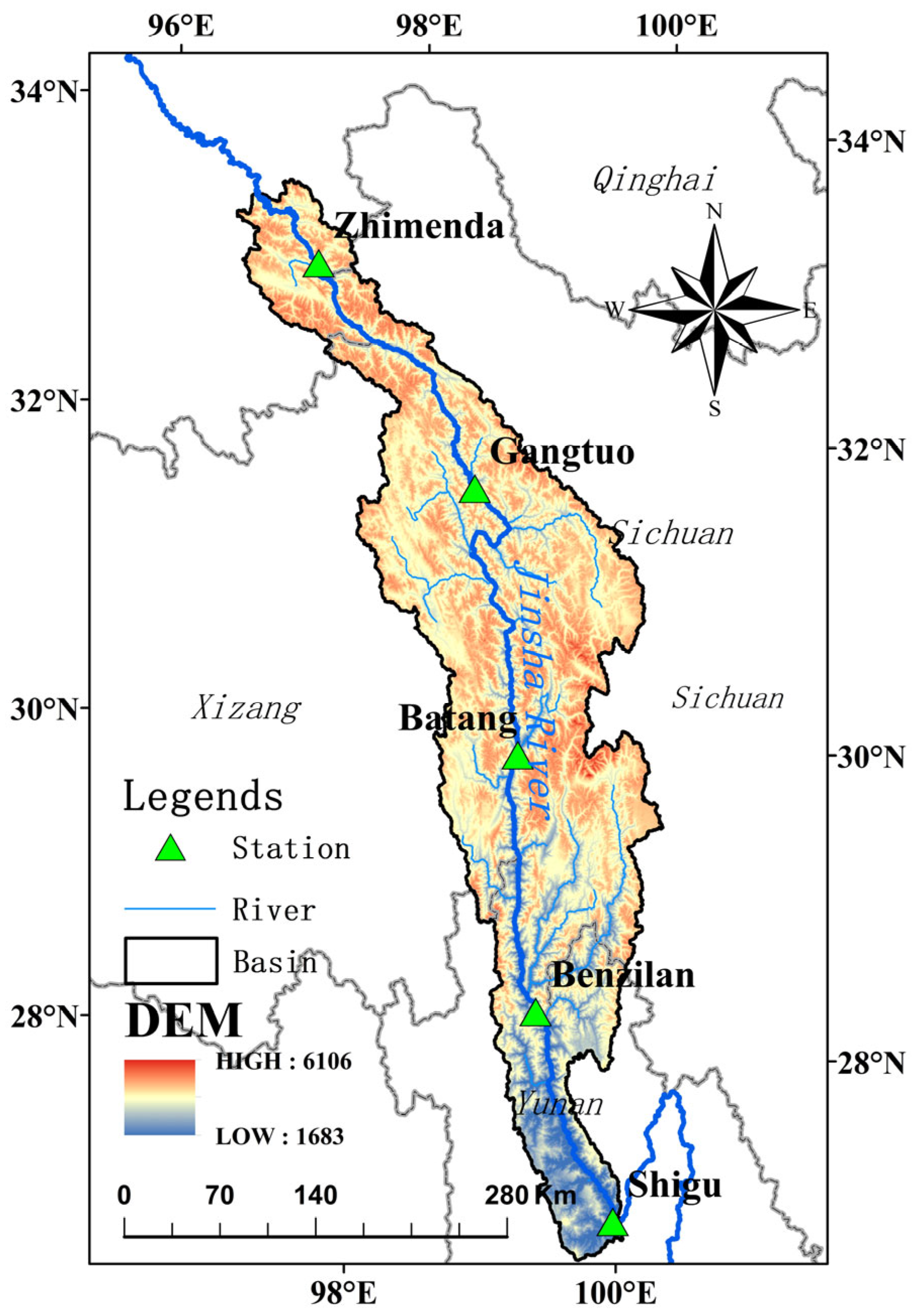
Figure 1. Schematic diagram of the location of the study area.
Water 17 03396 g001
Figure 2. Technical Roadmap.
Water 17 03396 g002
Figure 3. One-day (labeled as 1) and two-day (labeled as 2) upstream contributing areas for each hydrological station in the study area.
Water 17 03396 g003
Figure 4. Sample size at the annual scale.
Water 17 03396 g004
Figure 5. The daily runoff reconstruction sequence of (a) SG; (b) BZL; (c) BT; (d) GT; and (e) ZMD.
Water 17 03396 g005aWater 17 03396 g005b
Figure 6. Scatter plots of predicted versus observed daily streamflow on the test set for (a) BT; (b) BZL; (c) GT; (d) SG; and (e) ZMD. The 45° reference line indicates perfect agreement.
Water 17 03396 g006
Figure 7. The Accuracy, F1, Precision and Recall of the reconstruction results of both training and testing sets at each site under High Flow and Extreme High Flow.
Water 17 03396 g007
Figure 8. Line chart of reconstruction errors of the PSAL model under lag times T-1 to T-7 for each station.
Water 17 03396 g008
Figure 9. Runoff reconstruction simulation—measured scatter plot of SG, BZL, BT, GT and ZMD stations under different lag times (ae).
Water 17 03396 g009
Figure 10. Comparison chart of NSE and RMSE evaluations of LSTM-Baseline and PSAL models at five sites.
Water 17 03396 g010
Figure 11. Heat map of the ablation experiment results of meteorological characteristics at different stations.
Water 17 03396 g011
Table 1. PSAL model feature matrix.
Input DataStreamflow DataPrecipitationTemperatureWind SpeedSunshine DurationRelative Humidity
Number of
Input Days
711111
Number of Output Streamflow Days1\
Modeling
Approach
Multistep Forecasting
Simulation
Lag Time
Changes in dates with missing remote sensing data
Table 2. Statistical Table of Hyperparameter Settings for the PSAL model.
Hyperparameters in Stefenon et al., 2023 [47]Hyperparameters in This Study
Input Length24 h7 day
Loss FunctionMSEMSE
OptimizedADAMADAM
Learning Rate0.0010.0005
Epochs10010
Batch Size/32
Table 3. PSAL Evaluation of Runoff Reconstruction model.
Cross-SectionDatasetNSER2NRMSERelMAE
SGTraining set0.97 0.99 0.030.09
Testing set0.80 0.92 0.070.20
BZLTraining set0.97 0.99 0.030.09
Testing set0.83 0.93 0.060.20
BTTraining set0.95 0.98 0.020.16
Testing set0.89 0.94 0.210.72
GTTraining set0.95 0.98 0.030.12
Testing set0.71 0.85 0.130.28
ZMDTraining set0.91 0.95 0.020.16
Testing set0.83 0.92 0.080.26
Table 4. Evaluation of the LSTM-Baseline Runoff Reconstruction Model.
LSTM-BASELINENSER2RMSEMAE
BT0.210.67817.32431.07
BZL0.220.571134.12778.44
GT0.170.62599.73359.91
SG−0.270.461270.08763.11
ZMD0.040.56555.95386.51
Table 5. Evaluation of Meteorological Characteristic Ablation Experiment Results.
Cross-SectionRemoved FeatureNSEΔNSER2ΔR2RMSEΔRMSEMAEΔMAE
BT/0.8900.940308.760192.120
Precipitation_10.15−0.740.67−0.27846.4537.64471.83279.71
Wind_10.28−0.610.67−0.27780.27471.51428.74236.62
Temperature_10.36−0.530.75−0.19733.62424.86390.98198.86
Sunshine_10.21−0.680.65−0.29815.1506.34431.29239.17
Humidity_10.14−0.750.58−0.36851.69542.93450.85258.73
Precipitation_20.86−0.030.93−0.01348.6639.9210.4918.37
Wind_20.87−0.020.93−0.01334.225.44199.697.57
Temperature_20.28−0.610.71−0.23782.04473.28427.92235.8
Sunshine_2−0.09−0.980.41−0.53959.14650.38531.17339.05
Humidity_2−0.07−0.960.27−0.67951.91643.15577.07384.95
BZL/0.8300.930443.240288.440
Precipitation_10.76−0.070.92−0.0153086.76292.614.17
Wind_10.860.030.930411.12−32.12271.33−17.11
Temperature_10.79−0.040.930500.9157.67278.21−10.23
Sunshine_10.850.020.930422.76−20.48251.51−36.93
Humidity_10.81−0.020.92−0.01478.1734.93300.9412.5
Precipitation_20.76−0.070.89−0.04535.492.16300.0511.61
Wind_20.77−0.060.91−0.02521.6478.4299.9711.53
Temperature_20.850.020.92−0.01421.8−21.44248.96−39.48
Sunshine_20.74−0.090.92−0.01552.3109.06314.4426
Humidity_20.8300.930442.77−0.47269.41−19.03
GT/0.7100.850371.170185.220
Precipitation_10.63−0.080.82−0.03417.145.93224.1438.92
Wind_10.7100.850367.34−3.83188.363.14
Temperature_10.69−0.020.850379.658.48196.5611.34
Sunshine_10.7−0.010.84−0.01375.834.66193.918.69
Humidity_10.68−0.030.850389.7418.57210.7825.56
Precipitation_20.51−0.20.81−0.04480.43109.26266.3781.15
Wind_20.59−0.120.850439.5868.41243.5758.35
Temperature_20.65−0.060.83−0.02405.0433.87214.0428.82
Sunshine_20.720.010.850360.45−10.72184.8−0.42
Humidity_20.68−0.030.850389.4218.25212.0426.82
SG/0.800.920506.320267.830
Precipitation_10.79−0.010.89−0.03520.9414.62298.1630.33
Wind_10.69−0.110.920628.56122.24359.1491.31
Temperature_10.41−0.390.87−0.05867.09360.77463.36195.53
Sunshine_10.55−0.250.9−0.02758.77252.45466.73198.9
Humidity_10.48−0.320.86−0.06811.61305.29416.83149
Precipitation_20.46−0.340.91−0.01832.55326.23480.49212.66
Wind_20.68−0.120.930.01634.16127.84381.68113.85
Temperature_20.75−0.050.920567.8361.51322.3254.49
Sunshine_20.79−0.010.9−0.02512.486.16288.1520.32
Humidity_20.71−0.090.91−0.01604.9598.63346.6778.84
ZMD/0.8300.920232.690132.590
Precipitation_10.76−0.070.88−0.04277.845.11157.3824.79
Wind_10.8300.91−0.01234.361.67131.01−1.58
Temperature_10.73−0.10.920294.8962.2182.3349.74
Sunshine_10.8300.91−0.01236.443.75133.591
Humidity_10.74−0.090.87−0.05287.0854.39162.9630.37
Precipitation_20.840.010.920226.08−6.61139.847.25
Wind_20.8300.920230.84−1.85131.88−0.71
Temperature_20.82−0.010.91−0.01239.46.71146.9414.35
Sunshine_20.81−0.020.920246.8314.14136.844.25
Humidity_20.69−0.140.85−0.07316.8184.12176.5443.95
Disclaimer/Publisher’s Note: The statements, opinions and data contained in all publications are solely those of the individual author(s) and contributor(s) and not of MDPI and/or the editor(s). MDPI and/or the editor(s) disclaim responsibility for any injury to people or property resulting from any ideas, methods, instructions or products referred to in the content.