Article

Numerical Analysis of 3D Slope Stability in a Rainfall-Induced Landslide: Insights from Different Hydrological Conditions and Soil Layering

1
Zhejiang Institute of Hydraulics and Estuary (Zhejiang Institute of Marine Planning and Design), Hangzhou 310020, China
2
National Key Laboratory of Water Disaster Prevention, College of Hydrology and Water Resources, Hohai University, Nanjing 210098, China
3
Institute of Water and Environment, Karlsruhe Institute of Technology, 76131 Karlsruhe, Germany
4
Faculty of Engineering, China University of Geosciences (Wuhan), Wuhan 430074, China
5
School of Urban Construction, Wuhan University of Science and Technology, Wuhan 430065, China
*
Author to whom correspondence should be addressed.
Water 2025, 17(22), 3316; https://doi.org/10.3390/w17223316
Submission received: 12 October 2025 / Revised: 15 November 2025 / Accepted: 17 November 2025 / Published: 20 November 2025
(This article belongs to the Special Issue Water-Related Landslide Hazard Process and Its Triggering Events)

Abstract

The analysis of rainfall-induced landslides, which involve complex interactions between hydrology, soil mechanics, and geometry, is still limited by simplifying assumptions in existing models. We introduced a numerical model that couples soil infiltration with three-dimensional (3D) slope stability analysis. After validating against benchmark problems, we used this model to investigate the effects of various hydro-geotechnical conditions on slope stability. The results show that rainfall intensity dictates the stability of shallow landslides, while for deep-seated landslides, it governs the rate of progression toward failure. A high initial groundwater table reduces slope stability by accelerating soil weakening, particularly for deep landslides. Although upward moisture redistribution via matric suction is possible, its effect is negligible during infiltration, allowing deep saturation and landslide risk to persist. Furthermore, a low-permeability basal layer impedes drainage, leading to pore pressure buildup and a rapid decline in stability. The proposed model could potentially overcome the limitations in predictive accuracy of current hydro-geotechnical models arising from their oversimplified representations.

1. Introduction

Landslides occur frequently worldwide, causing thousands of fatalities each year and inflicting both direct and indirect damage to urban infrastructure and private property [1]. These events generate annual economic losses estimated in the billions of dollars [2,3]. Among the various types of landslides, rainfall-induced soil landslides are the most widespread. Rainfall, as a common natural driver, initiates hydrological processes that significantly alter soil moisture and mechanical properties, playing a key role in triggering both shallow and deep-seated soil failures [4].
The spatiotemporal distribution of soil moisture within a watershed is mainly governed by rainfall-driven hydrological processes, including infiltration, surface runoff, and subsurface flow. The dynamics of these processes are, in turn, controlled by the interplay between meteorological inputs and geohydrological characteristics of hillslopes [5]. This interaction can alter the soil mechanical properties, ultimately creating the preconditions for failure initiation [6,7]. Physically and process-based approaches are widely used due to their ability to offer deep mechanistic insights into how key processes directly influence the forces acting on a slope, e.g., rainfall infiltration, pore water pressure evolution, and soil suction [8,9,10]. While both hydrological and slope-stability models have achieved significant progress as independent fields, the coupled application of these approaches is fundamentally constrained by the underlying assumptions concerning the interplay of soil water flow, soil stress, and slope stability [11,12,13]. Minor deviations in these assumptions (e.g., problem dimensionality or the translation of pore pressure to stress) or input parameters could substantially alter model outputs. While such models demonstrate “validity” within specific evaluative contexts, particularly in regional-scale applications [14,15], they may obscure the precise triggering mechanisms of landslides.
Coupling rainfall infiltration with slope stability analysis bridges the gap between hydrological processes and landslide hazards. While the theories of infiltration [16,17] and slope stability [18] were initially developed independently, a comprehensive theoretical framework was proposed by [19]. This framework provides critical insights into how hydrologic processes influence the location, timing, and rate of landslides, and offers a basis for anticipating landslide hazards in response to transient infiltration and groundwater pressures. Although significant progress has been made in hydrological–geotechnical modeling in recent years, with simulation scales extending from the hillslope to the catchment or even regional level, the existing simulation tools remain limited in several aspects: (i) Most current models solve the limit equilibrium equation based on the infinite-slope (1D) assumption (e.g., TRIGRS [10] and GEOtop-FS [20]), which fails to capture the complex geometries of real-world slope failures; (ii) Three-dimensional approaches, such as Scoops3D [21] and r.slope.stability [22], are typically applicable only under static conditions, including imposed water levels or fully saturated soil states; (iii) Some models consider only total soil water storage rather than the vertical distribution of soil moisture (e.g., iCRESTRIGRS [2] and SHIA_Landslide [23]) within their hydrological submodules. Thus, there is still a notable lack of integrated frameworks capable of coupling dynamic soil-water processes with 3D slope stability analyses, which are essential for accurately transferring spatiotemporal variations of pore water pressure and soil stress across potential slip surfaces.
While the role of pore water pressure and its gradient in slope failure is well understood, the specific hydrological processes that trigger landslides remain difficult to isolate [6]. Commercial geotechnical software, such as PLAXIS 2024.3 [24] and GeoStudio 2024.1, provide robust and mature solutions for coupled flow-deformation analyses. However, they often suffer from (i) limited flexibility for customized research scenarios and batch parameter studies, and (ii) dimensional or computational limitations in accurately modeling 3D slope stability under rainfall-induced infiltration. Although the influences of rainfall intensity [25,26,27], soil properties [28], and soil and/or hydrological conditions [29] have been extensively investigated in previous studies, these works primarily focus on shallow landslides, with limited attention to deep-seated or fully three-dimensional landslide processes. Because most existing studies are region-specific, there remains a lack of systematic analyses based on controlled numerical experiments. Consequently, the experimental conditions in such studies tend to be relatively isolated, with few attempts to explore the combined effects of multiple factors. This situation arises not only from the structural limitations of current models and the dimensional constraints of their governing equations, but also from the increasing demands placed on model verification, robustness, and flexibility.
To address these challenges, we developed a coupled framework integrating rainfall infiltration, soil mechanics, and three-dimensional slope stability, resulting in a numerical model for simulating rainfall-induced slope failure. After validating the model through a series of benchmark tests, we conducted numerical experiments to systematically investigate the influence of rainfall intensity, initial conditions, soil properties, boundary conditions, and landslide geometry on slope stability. Section 2 presents the theoretical foundations of the model, including formulations for soil water flow, soil stress, and slope stability. Model validation and analysis are provided in Section 3. Section 4 outlines the numerical setup and experimental design, followed by results in Section 5. Section 6 offers a discussion of the findings, and Section 7 presents conclusions.

2. Model Theory

2.1. Soil Water Flow

The movement of water in soil is primarily governed by gradients in potential energy. For one-dimensional vertical flow, soil water movement is typically described using Darcy’s law:
q = K ( h ) ( h + z ) z
where q is the unit-width flux of soil water, K ( h ) is the hydraulic conductivity, h is the pressure head (pore water pressure), and z is the vertical height in the soil profile. For any soil element, based on the continuity equation of water balance (neglecting source and sink terms):
θ t = q z
where θ is the volumetric water content of the soil, and t is time. By combining Equations (1) and (2), we obtain the governing equation for water flow applicable to various soil saturation levels, known as the classical Richards equation [30]:
θ t = z K ( h ) h z + 1
Solving the Richards equation requires introducing the soil-water characteristic curve. We employed the classical Mualem–Van Genuchten function [31,32], which has been widely used across various regions worldwide and is recognized as the foundation of several international databases [33]. θ ( h ) can be expressed as the following equation, as derived from Van Genuchten [32]:
θ = θ r + θ s θ r 1 + | α h | n m
where θ s is the saturated water content of the soil, θ r is the residual water content in the dry soil state, and α , n, and m are empirical parameters that define the shape of the curve. The parameter m can be computed as m = 1 1 / n . Substituting this relation into Mualem’s expression for unsaturated hydraulic conductivity gives:
K = K sat S e λ 1 1 S e 1 m m 2
where K sat is the saturated hydraulic conductivity, λ is an empirical parameter related to the tortuosity of infiltration flow (typically 0.5), and S e , the relative saturation, is given by:
S e = θ θ r θ s θ r
To construct a numerical scheme for Equation (3), the expression for θ must be transformed into the soil water capacity C:
C = θ h = α m n | α h | n 1 θ s θ r 1 + | α h | n ( m + 1 )
To obtain a steady-state numerical solution for Equation (3), the hydraulic conductivity must be treated implicitly using its derivative form, d K / d h . Additionally, a modification of the relative saturation near full saturation is required [34]. This modification introduces a small capillary height, h e (interpreted as an air entry value), and alters the soil water retention curve [35]. This study adopts the relative saturation, proposed by Ippisch et al. [36]:
S e = 1 S c 1 + | α h | n m h < h e 1 h h e
where S c corresponds to the relative saturation at the cutoff value h e , given by S c = 1 + α h e n m . Consequently, the soil permeability is given by:
K = K sat S e λ 1 1 S e S c 1 / m m 1 1 S c 1 / m m 2 S e < 1 K sat S e 1
When h e = 0 , the modified S e and K revert to Equations (4) and (5). Existing studies suggest that these modifications have a minimal impact on the soil characteristic curve but may significantly affect the unsaturated hydraulic conductivity of fine-textured soils [34,35,36]. To ensure numerical stability, cubic spline approximations are applied in regions where h < 0.01 and h > 1.05 h e to maintain the continuity of the soil-water retention curve and the soil water capacity function, C. Equation (3) is solved using the classical finite difference method, following the approach from van Dam et al. [37] in the SWAP model’s soil-water module. An implicit backward difference scheme is employed:
θ i j + 1 h i j + 1 , p + 1 θ i j = Δ t j Δ z i K i 1 / 2 j h i 1 j + 1 , p + 1 h i j + 1 , p + 1 1 / 2 Δ z i 1 + Δ z i + K i 1 / 2 j K i + 1 / 2 j h i j + 1 , p + 1 h i + 1 j + 1 , p + 1 1 / 2 Δ z i + Δ z i + 1 K i + 1 / 2 j
where the superscript j denotes time, the subscript i denotes the vertical spatial index, and the superscript p denotes the iteration step. Δ t j = t j + 1 t j is the time discretization, and Δ z i is the vertical soil layer discretization. More detailed descriptions of the numerical scheme can be found in the literature [37].

2.2. Soil Effective Stress

The essence of slope instability induced by hydrological processes lies in the change in soil shear strength caused by variations in soil moisture. Based on the theories of Terzaghi and Bishop, Lu and Likos [38] refined the expression for effective stress, σ , as:
σ = σ u a σ s
where σ is the total stress, u a is the soil air pressure, and σ s is the soil suction stress. The general expression for σ s , applicable to both unsaturated and saturated states, is:
σ s = u a u w u a u w 0 σ s = f u a u w u a u w 0
where u a u w represents the matric suction, and the function f describes the relationship between matric suction and suction stress. Lu et al. [39] established a closed-form solution for soil shear stress based on van Genuchten’s soil-water characteristic curve (SWCC):
σ = σ u a + u a u w u a u w 0 σ = σ u a + u a u w 1 + α u a u w n ( n 1 ) / n u a u w 0
When soil pore air pressure is neglected ( u a = 0 ), matric suction u a u w can be expressed in terms of pressure head as:
u a u w = γ w h
where γ w is the unit weight of water. By computing the pressure head h obtained in the previous section, the soil water content θ and suction stress can be determined, thereby establishing the complete soil water characteristic curve (SWCC) and soil suction stress characteristic curve (SSCC). These two relationships form the fundamental theoretical basis for linking hydrological processes to slope stability analysis.

2.3. 3D Slope Stability

We employed the three-dimensional limit equilibrium Hovland model [40] for the evaluation of soil stability. The model discretizes the slope into soil column elements (see Figure 1a), and the dynamic soil moisture and stress are computed for each element. Following a force equilibrium analysis, the overall safety factor F s is obtained by summation, representing the ratio of resisting forces to driving forces along the sliding surface (see Figure 1b):
F s = c c s · A + G cos β c σ s · A tan ϕ cos β m c G sin β m cos β m
where c s denotes soil cohesion; ϕ is the internal friction angle of the soil; G represents the soil weight; β c and β m correspond to the inclination angle and apparent inclination angle of the soil column, respectively; and A denotes the sliding area of the soil. Under rainfall infiltration and gravitational forces, soil pores gradually become saturated with water, resulting in an increase in the soil weight G . Simultaneously, the SSCC relationship indicates that variations in soil moisture content induce changes in suction stress σ s . Consequently, these modifications in soil properties reduce the internal frictional resistance against sliding, potentially leading to slope failure ( F s < 1 ).
The coupled infiltration-stability modeling requires handling of multiple coordinate systems (see Figure 1a), including the global mapping coordinate system ( x , y , z ) , the local Cartesian coordinate system of the ellipsoid ( x , y , z ) , and the ellipsoid-aligned coordinate system ( x , y , z ) . The geometric transformations and derivations for these coordinate systems have been comprehensively detailed by Chen et al. [13]. Computational simulations typically assume curved sliding surfaces, since most observed landslides exhibit irregular shapes. Currently, the ellipsoidal assumption is widely adopted, and some studies have shown satisfactory results using this approach [41,42]. The ellipsoidal assumption employs multiple geometric parameters (e.g., semi-major and semi-minor axes) to flexibly characterize various landslide morphologies while maintaining reasonable computational costs. In practical calculations, the lower boundaries of soil column elements (see Figure 1) approximately form the ellipsoidal sliding surface, with the approximation improving as mesh resolution increases. Under the influence of slope gradient and aspect, each landslide surface possesses distinct values of A, β c , and β m , consequently requiring force calculations in both the normal and sliding directions based on different angles (see Figure 1).

3. Validation and Analysis

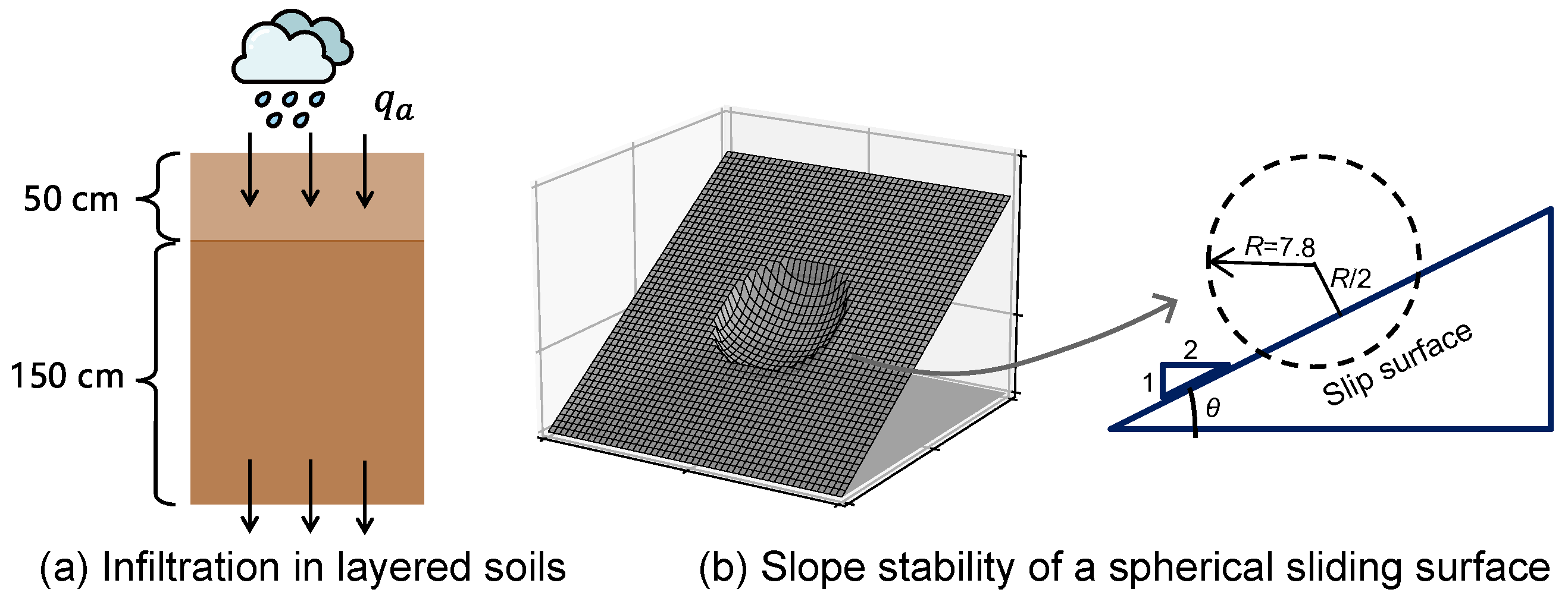
Based on the structure of the coupled model, this study aims to validate not only its individual submodules but also the effectiveness of the coupling mechanism between soil moisture and stress. Therefore, we will examine the soil infiltration process, the three-dimensional slope stability model, and the coupling behavior using the soil-water characteristic curve (SWCC) and the soil suction stress characteristic curve (SSCC) in the following sections. We validated the infiltration-stability method through simulations of benchmark problems (see Figure 2), encompassing both the infiltration process and slope stability analysis. We employed three representative soil types in the validation tests: sand, loam, and clay, with their key parameters listed in Table 1. The hydraulic properties are determined according to the soil texture classes from the HYDRUS-1D (version 7.0) software soil catalog [43]. Additional parameters, including soil porosity ( n p ) and dry unit weight ( γ s ), are obtained from the Harmonized World Soil Database (HWSD v1.2) [44].

3.1. Validation of Variably Saturated Subsurface Flow

For one-dimensional flow based on Richards’ equation, we compared the numerical model results with analytical solutions under specific initial and boundary conditions. Thus, we applied our method to two classical benchmark problems: (i) rainfall-induced variations in soil profile moisture [45], and (ii) the Warrick problem [46] with a fixed pressure head. These problems have been widely used to validate Richards equation solvers, as analytical solutions are available [47,48]. For the first case (steady-state flow under constant precipitation) with free drainage at the lower boundary, Vanderborght et al. [45] provided the analytical solution. The boundary and initial conditions are specified as:
K + K h z z = 0 = q a ( h + z ) z z = bot = 1 h t = 0 = h 0
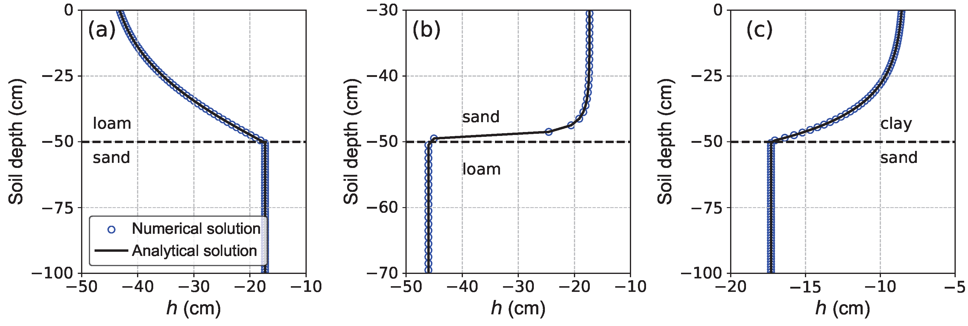
The total soil depth is 200 cm, divided into two layers filled with different soil types: an upper layer of 50 cm and a lower layer of 150 cm. The precipitation rate is set to q a = 0.5 cm · d 1 , with initial conditions of h ( z , t = 0 ) = 200 cm . The vertical spatial discretization, Δ z , along the soil depth is 1 cm. Under these conditions, the soil moisture content reaches steady-state values after sufficient simulation time. Figure 3 presents the steady-state soil pressure head (h) profiles under the aforementioned conditions for multilayered soils, comparing numerical simulations with analytical solutions. Since the saturated hydraulic conductivity of all three soil types exceeds the precipitation rate, no surface runoff occurs. The results show nearly identical pressure head profiles between the numerical and analytical solutions, confirming the rationality and accuracy of the numerical model.
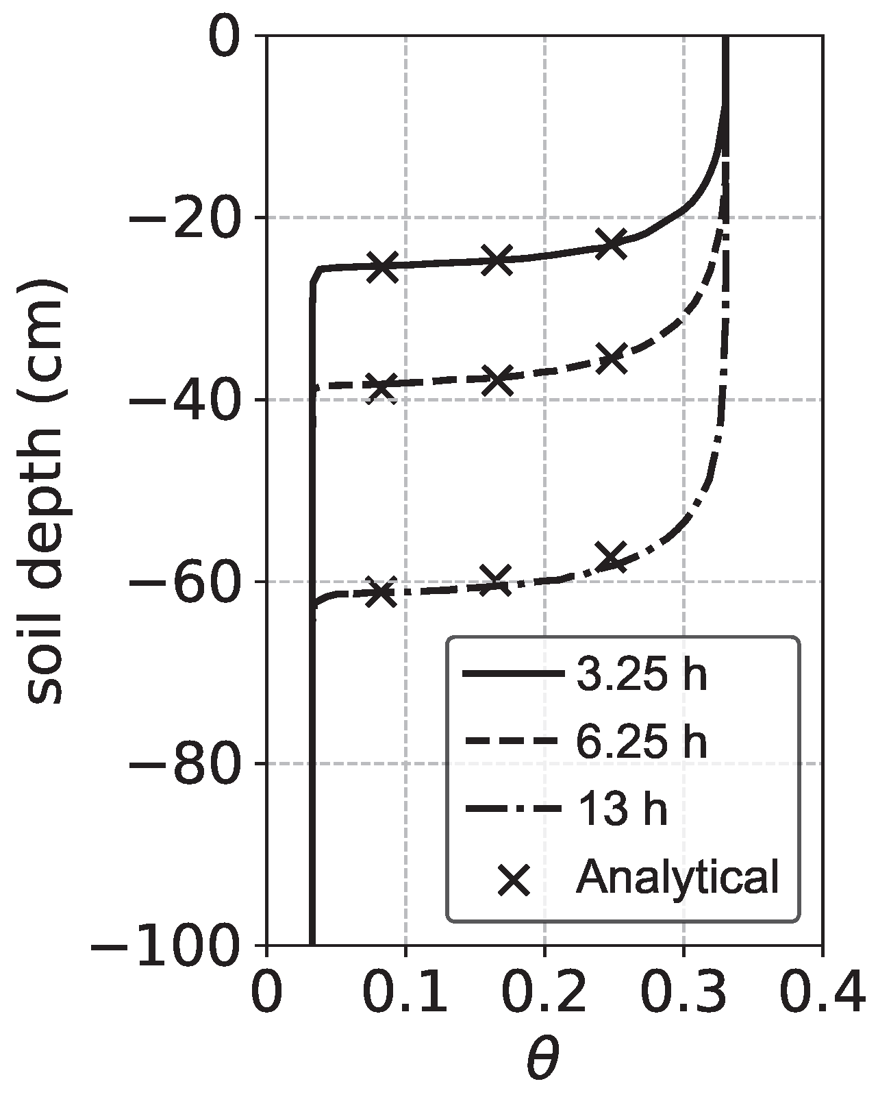
In the Warrick problem, a fixed pressure head of 0 cm is applied to the top of a soil column. The column is initially nearly dry, with a uniform water content of 0.03. A Neumann boundary condition (no-flow) is imposed at the bottom of the domain. The soil parameters used in the Warrick problem are as follows: θ r = 0 , θ s = 0.33 , K sat = 24.97 cm · d 1 , α = 0.0143 , and n = 1.56 . The same grid resolution as in the previous case was applied. As shown in Figure 4, the numerical model achieves good agreement with the analytical solution.

3.2. Validation of the Slope Stability

We validated the slope stability model using an idealized landslide scenario by computing the factor of safety ( F s ) for a spherical sliding surface (see Figure 2b). The geometric and material parameters were defined as follows: sphere radius R = 7.8 m , slope angle θ = 26.6 ° ( tan θ = 0.5 ), unit weight γ s = 9.8 kN / m 3 , friction angle ϕ = 0 , and cohesion c s = 7.644 kPa . We selected these parameters to match previous benchmark studies [41,49,50,51]. We employed a grid resolution of Δ x = Δ y = 1 m . As shown in Table 2, the computed F s values exhibit close agreement with reference solutions. Minor discrepancies observed are attributed to differences in numerical implementation and discretization schemes. This comparison confirms the validity of the proposed model for slope stability analysis.
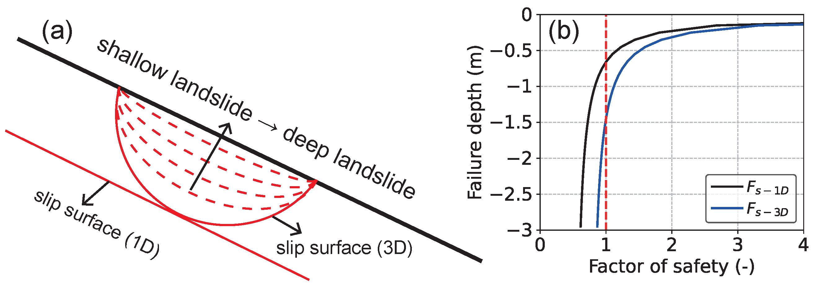
We also compared the differences between the three-dimensional (3D) and one-dimensional (1D) models in evaluating slope stability. Figure 5a illustrates the contrast between the two approaches in representing slope geometry. In the 3D model, the sliding surface is defined as the intersection between the ellipsoid and the incline, whereas in the 1D model, it is represented by an infinite slope parallel to the ground surface. Using the same soil parameters listed in Table 2, we gradually reduced the length of the minor semi-axis of the ellipsoid to simulate landslides of varying depths. For each specified landslide depth, we computed the corresponding F s ; the maximum depth of the 3D slope was set equal to that of the infinite slope. As shown in Figure 5b, the 1D model generally produced more conservative results—lower F s values, indicating poorer stability—across most depths. This finding aligns with observations reported in previous studies. Notably, the results of the two models converge for shallower landslides because, at reduced depths, the conditions approach the assumptions of an infinite slope and the 3D effects become less significant. This convergence also supports the validity of the proposed 3D method.

3.3. Coupled Response of Soil Water and F s

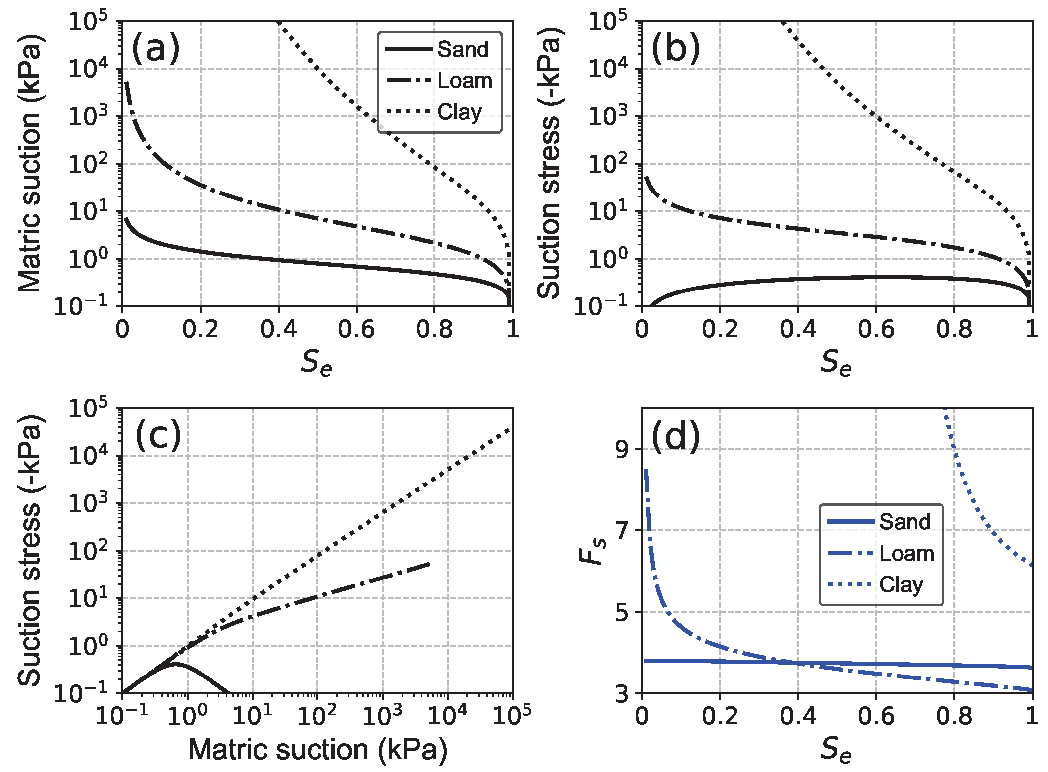
We further analyzed the variations in matric suction, suction stress, and the factor of safety ( F s ) with respect to changing effective saturation ( S e ). Figure 6 illustrates these relationships during the wetting stage. As no theoretical or reference solutions exist for direct comparison, this verification relies on analytical consistency checks. The matric suction of clay exhibited the most pronounced variation with S e , reaching extremely high values under dry conditions (see Figure 6a). In contrast, sand showed minimal matric suction variation, attaining only approximately 10 kPa even in the dry state. Loam displayed intermediate behavior in matric suction variation. All three soil types lost their matric suction completely upon full saturation ( S e = 1 ). The suction stress characteristics (see Figure 6b,c) of clay and loam followed trends similar to their matric suction, with values decreasing monotonically as S e increased. Sand, however, exhibited distinct suction stress behavior, peaking at intermediate saturation levels ( 0 < S e < 1 ). This phenomenon is primarily governed by the parameter n in the van Genuchten model.
Due to sand’s relatively stable suction stress across moisture variations, its factor of safety ( F s ) decreased only slightly with increasing effective saturation ( S e ) (see Figure 6d). For loam, F s declined rapidly during the initial wetting stage ( S e < 0.2 ), driven by significant suction stress loss, followed by a more gradual reduction until reaching its minimum at full saturation. Clay exhibited the most dramatic variation in F s : its high suction stress under dry conditions resulted in exceptionally large F s values, while its inherent cohesion maintained residual stability even at full saturation.

4. Numerical Experiments Setup

We conducted numerical experiments to simulate slope stability using realistic soil parameters derived from rainfall-induced landslide events. As detailed in Table 3, the soil parameters were derived from field measurements reported in the literature [53,54], corresponding to 140 landslides and 33 debris flow events triggered by persistent heavy rainfall during the summer of 2011. These parameters, derived from field observations or experimental studies of actual landslides, indicate that their physical characteristics accurately represent the soil properties when the slope is in an unstable state. Therefore, such data provide a more realistic reflection of the actual landslide mechanisms than do idealized or empirically derived parameters. Note that more detailed geotechnical factors, such as soil fissures, lithology, and soil biota, are not considered in this study.
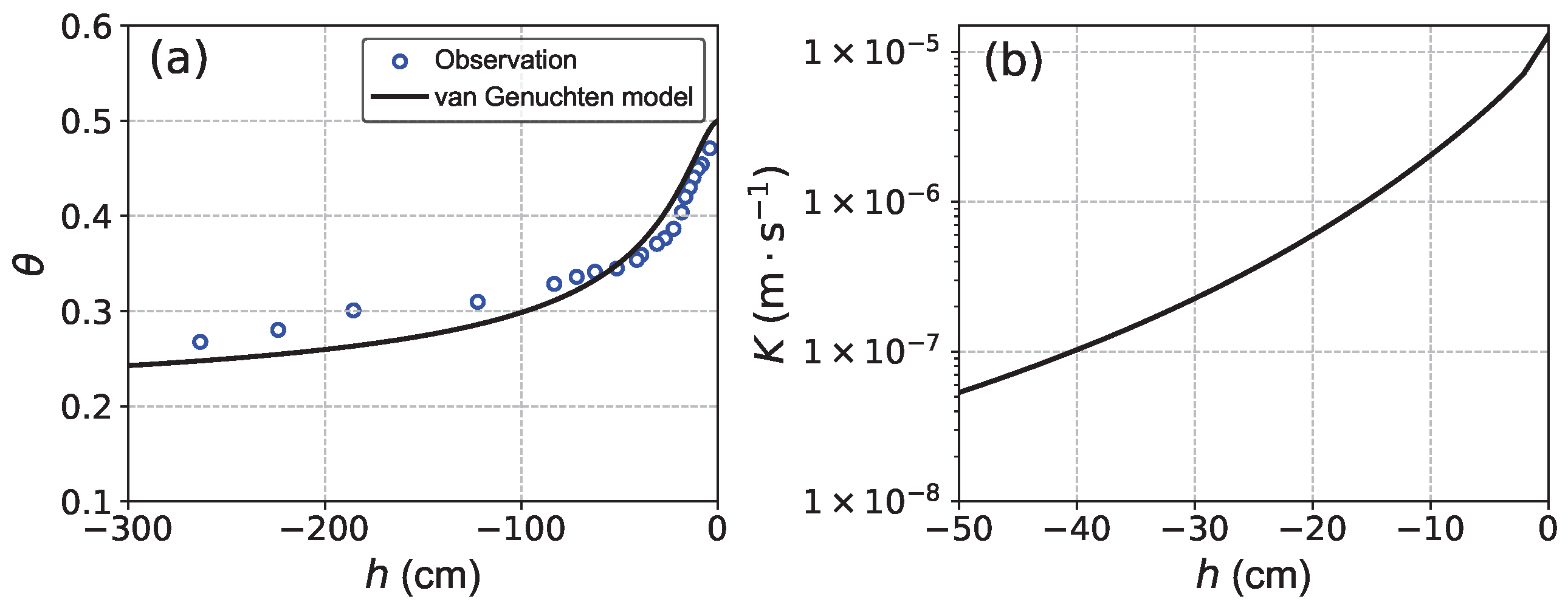
Figure 7 presents the soil-water retention curves fitted using the van Genuchten model with parameters from Table 3. The results confirm that the van Genuchten model effectively captures the moisture variation characteristics of these soils. To simulate a layered soil scenario, we introduced an additional, less permeable soil type (S2 with K sat = 112.32 cm · d 1 ) while keeping the other hydraulic parameters identical to those of the original soil (S1).
The simulated cases examined variations in soil type, hydrological initial and boundary conditions, and rainfall intensity (see Table 4). Specifically, we compared homogeneous and layered soil configurations. We define the initial conditions by the groundwater level (GWL, Table 4), ensuring hydrostatic equilibrium of soil moisture along the depth at t = 0 . We tested the bottom boundary conditions under both free drainage and zero-flux scenarios. Rainfall intensities were scaled relative to K sat and applied continuously throughout the simulation. This normalized approach highlights the relationship between rainfall input and soil infiltration capacity, making the results more general and comparable across different soil types. In addition, the simplification was made to focus on the hydrological and mechanical responses of the slope under different rainfall magnitudes and durations, while avoiding additional uncertainties associated with complex temporal variations of natural rainfall.
For all cases, the landslide geometry was modeled as an ellipsoid with three principal dimensions: the major semi-axis a e (fixed at 10 m), the minor semi-axis b e (fixed at 6 m), and the failure depth c e (varied as 1, 2, 3, and 4 m to represent different landslide thicknesses). The setup of soil thickness ensures that the model can capture the dynamics of both shallow and deep landslides. The slope had a 30 inclination, with its dip direction aligned along the major axis ( a e ). The spatial resolution was uniformly set to Δ x = Δ y = 1 m .

5. Results

5.1. Effect of Rainfall Intensity on Slope Stability

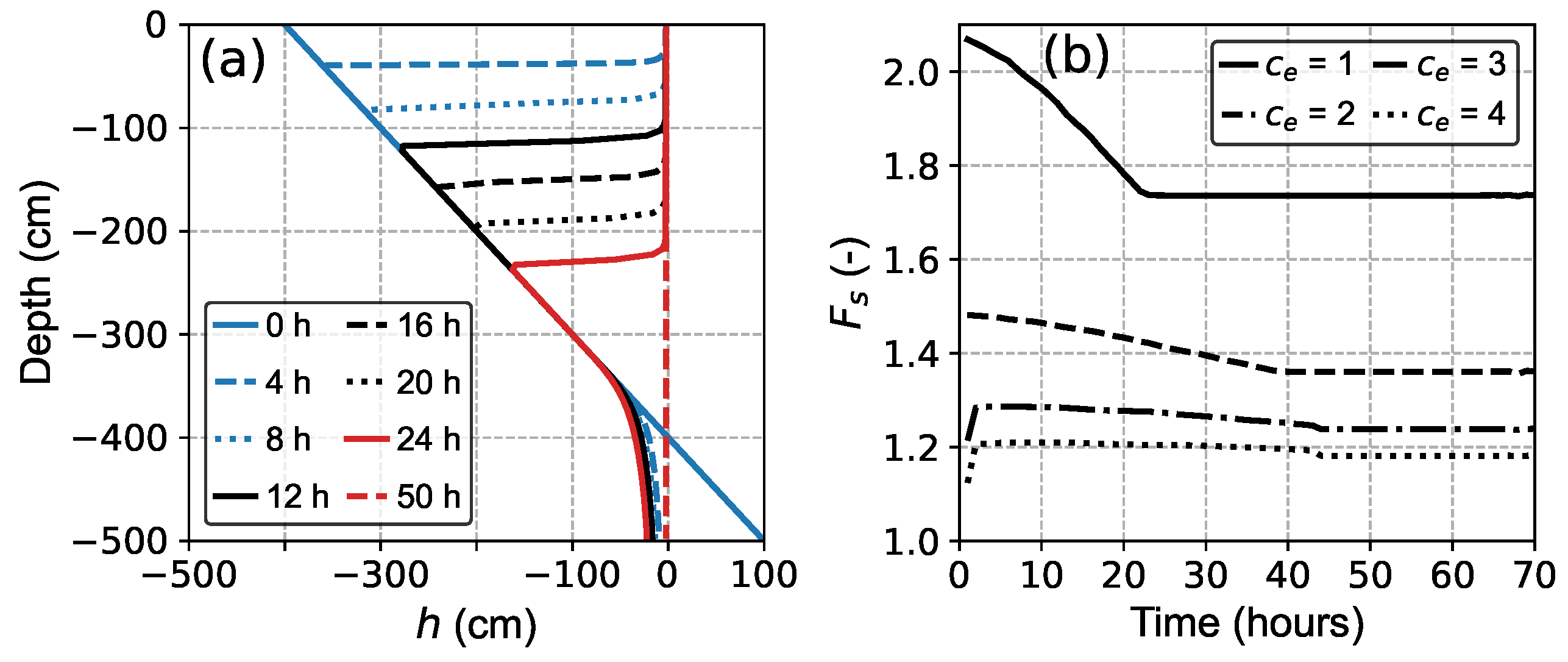
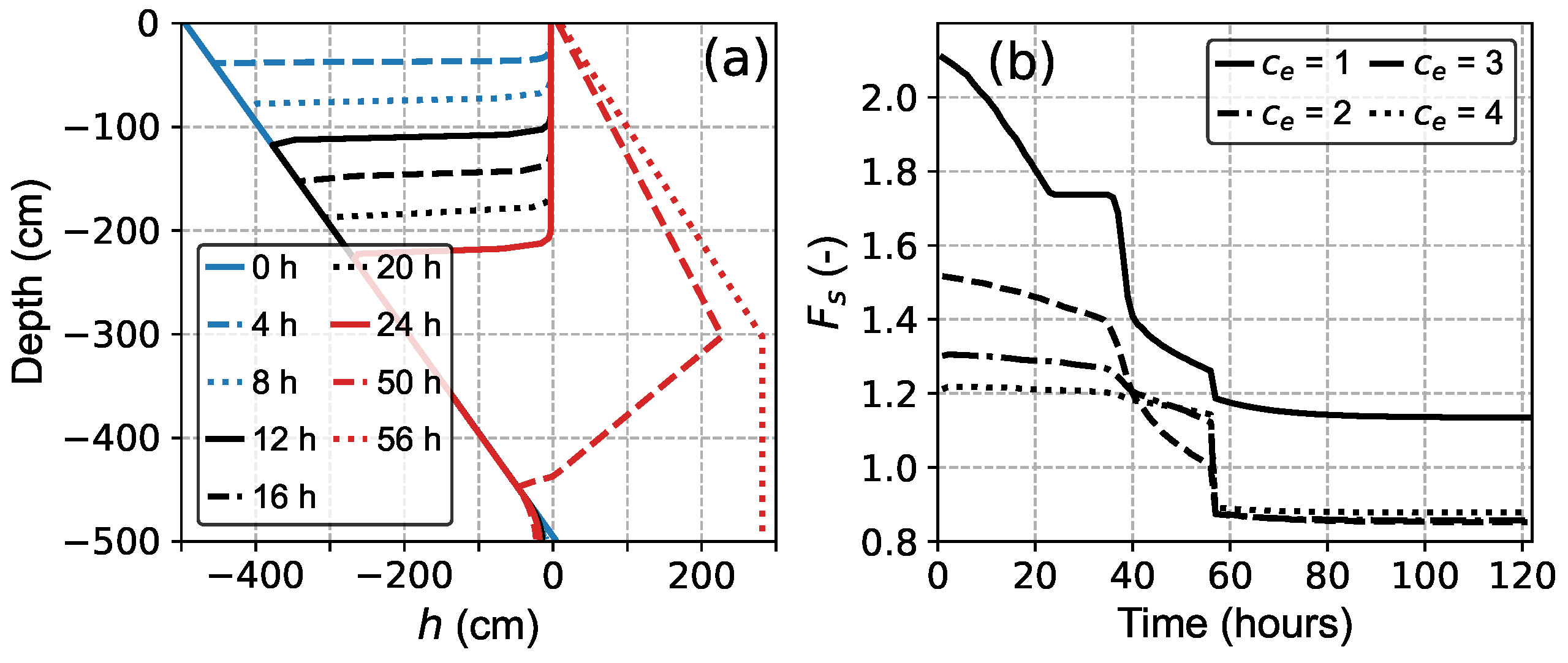
Cases 1, 2, and 3 examined the effects of rainfall intensity on slope stability, with values ranging from 0.5 K sat to 1.5 K sat . Figure 8 presents the temporal evolution of pore water pressure distribution under rainfall intensity 0.5 K sat . As shown in Figure 8a, the upper soil layer reached saturation first ( h = 0 ). At t = 8 h, approximately the upper 100 cm of soil became fully saturated, while pore water pressures in deeper layers remained similar to initial conditions ( t = 0 h), with maximum values around 400 cm. Under steady rainfall, pore water pressure evolved gradually, with complete profile saturation occurring at t = 50 h. For Case 2 with higher rainfall intensity ( 1.0 K sat ), the evolution of saturation pattern remained relatively uniform but accelerated significantly (Figure 8c). By t = 8 h, saturation extended to 150 cm depth, and near-complete saturation was achieved by t = 24 h (i.e, half the time required in Case 1). When intensity increased to 1.5 K sat (Case 3), we found the similar distributions to Case 2 (see Figure 8e). However, once rainfall intensity exceeded the saturated hydraulic conductivity, additional water failed to infiltrate deeper layers, instead forming surface ponding that generated positive pore water pressures ( h > 0 ) in upper soil layers.
In all cases, the F s decreased gradually during infiltration, converging to a steady-state value as the system reached equilibrium (see Figure 8b,d,f). The sensitivity of F s to rainfall diminished with increasing landslide thickness ( c e ), as shallow landslides exhibited more pronounced pore water pressure variations and faster responses to rainfall. Moreover, the time required for F s to converge increased with c e , reflecting delayed responses in deeper layers. This relationship was nonlinear—for instance, the convergence times for c e = 3 m and c e = 4 m were nearly identical, since thicker landslides have failure surfaces extending into deeper strata where pore pressure changes minimally affect F s . Comparison of Figure 8b,d shows that increasing intensity to 1.0 K sat accelerated F s convergence by approximately 10 h for shallow landslides ( c e = 1 m) and 20 h for deeper ones, demonstrating that higher intensities promote faster soil-water flux equilibration. In Case 3 ( 1.5 K sat , Figure 8f), F s evolution initially matched Case 2 trends but showed continued reduction beyond 10 h due to surface ponding. This effect also caused slightly greater F s reductions in deep landslides compared to Case 2. Lastly, F s converged at marginally lower values across all thicknesses when surface ponding and drainage reached balance.

5.2. Effect of Initial Conditions on Slope Stability

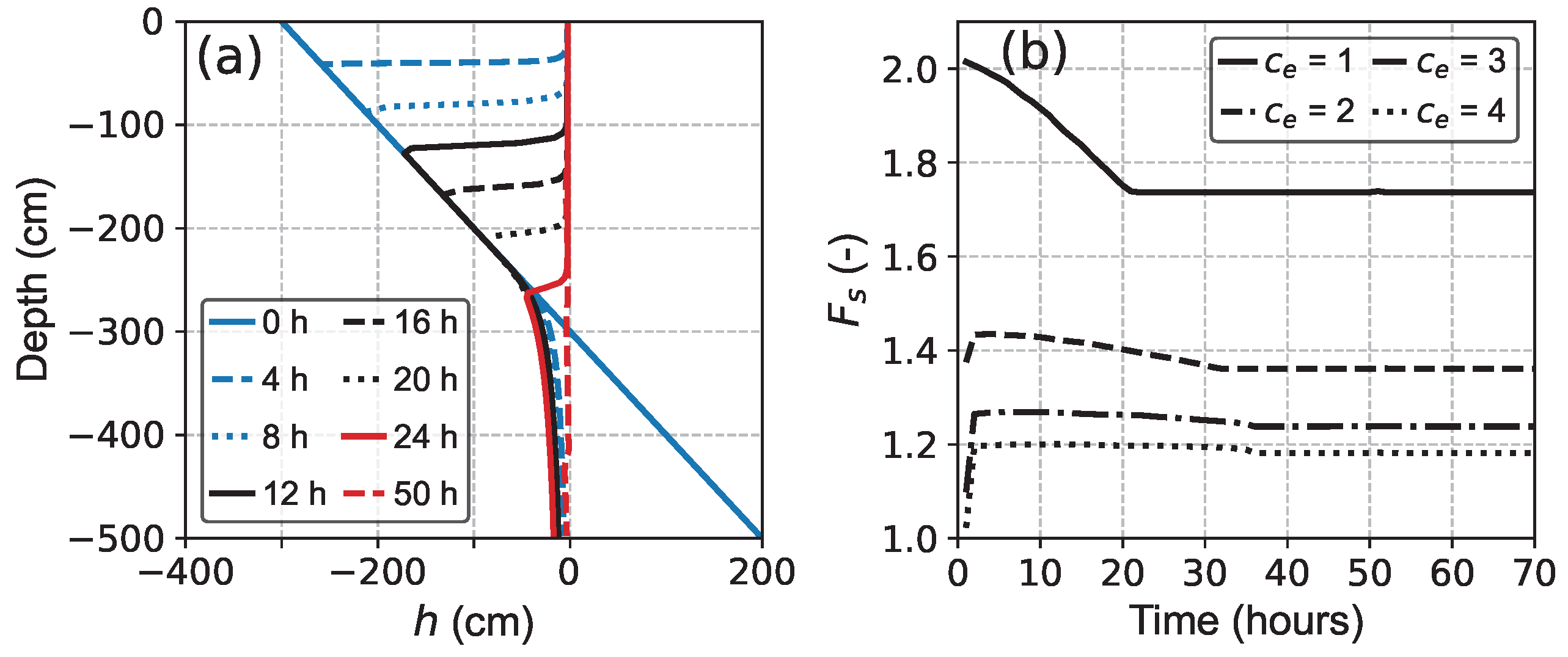
The comparative analysis of simulation results from Cases 1, 4, and 5 quantifies the influence of initial conditions. When the initial water table was raised from 500 cm to 400 cm (see Figure 9a) and 300 cm (see Figure 10a), the initial hydrostatic equilibrium of the soil profile was disrupted, resulting in elevated pore water pressures throughout the soil column. In these scenarios, the lower soil layer was saturated at the initial state. Following the onset of rainfall, the lower soil layer in Cases 4 and 5 transitioned to unsaturated conditions to accommodate the free drainage boundary condition. Compared to Case 1, the elevated initial water table did not substantially accelerate the wetting of the surface soil under identical rainfall conditions, yielding only marginal improvements in the downward propagation rate of saturation fronts. However, the raised water table maintained the lower soil layer in a near-saturated state from the onset of rainfall, thereby sustaining a substantially higher average soil moisture content throughout the rainfall event. This influence was particularly evident in the earlier development of positive pore water pressures across the soil profile.
Figure 9b and Figure 10b illustrate the slope stability evolution for Cases 4 and 5, respectively. Comparative analysis with Figure 8b reveals distinct patterns in slope stability responses to varying initial groundwater conditions. Shallow landslides exhibited minimal sensitivity to initial groundwater levels, with only slight variations in the F s at t = 0 h , attributable to differences in the initial h. In contrast, deep-seated landslides displayed a pronounced dependence on the initial water table elevation. Specifically, the time to convergence of F s decreased progressively with increasing initial water table height, advancing by approximately 5 h in Case 4 and 10 h in Case 5. This temporal shift is attributed to the expedited saturation of deeper soil layers facilitated by higher initial water tables. A notable phenomenon was observed in Case 4, where landslides with critical slip surfaces at c e = 3 m and c e = 4 m initially experienced an increase in stability, followed by a gradual decline. This non-monotonic behavior resulted from unsaturated hydrodynamic processes, wherein the saturated lower layers initially recharged the upper soil layers, thereby lowering h values, before eventual full saturation occurred under continued rainfall infiltration. When the water table was raised further in Case 5, this two-stage stability response extended to shallower landslides ( c e = 2 m ), indicating that sufficiently high initial water tables can influence the stability of even relatively shallow slope failures.

5.3. Effect of Soil Layers on Slope Stability

The S2 setup represents reduced permeability in the lower soil layers, reflecting gravitational effects in natural environments. Figure 11a shows the pore water pressure results for Case 6. Compared to Case 1 under identical hydrological conditions, we observed no difference in the upper soil layer during the initial rainfall period. As rainfall continued, the wetting front gradually advanced downward through the soil profile. Upon reaching the S2 layer (Figure 11a at t = 34 h), water accumulation occurred in the overlying S1 layer ( h > 0 ) due to the lower permeability of the underlying soil. Although the lower boundary of the S2 layer continued to drain at its permeability-controlled rate, limited drainage efficiency led to further water accumulation within the soil profile ( t = 50 h). At equilibrium ( t = 56 h), the system reached a steady state, with outflow occurring at the S2 layer’s saturated hydraulic conductivity, K sat . The hydraulic head gradient within the S2 layer vanished, while a linear distribution of h was observed in the S1 layer. This pattern arose because, in the saturated state, water in the S1 layer developed a reverse gradient to reduce the downward flow rate to match the lower K sat of the S2 layer.
The comparison of Figure 8b and Figure 11b reveals that the slope stability evolution in Case 6 is more complex. For shallow landslides, we identified six distinct stages. In the first stage, conditions resemble those of Case 1, with stability decreasing rapidly during the initial rainfall period. The second stage shows a plateau in stability similar to that observed in Case 1. However, after approximately 10 h at this plateau, F s declines sharply again, primarily due to water accumulation in the upper soil layer, which reduces internal friction resistance. During the fourth stage, F s decreases gradually as water accumulates in the lower soil layer. In the fifth stage, immediately prior to the final steady state, the rapid disappearance of the head gradient in the lower soil layer causes a sharp drop in F s . After roughly 60 h, slope stability reaches its final stable phase, with F s values lower than those in Case 1.
In contrast, deep-seated landslides undergo three distinct phases of decline. Initially, the decrease in F s mirrors the trend in Case 1 during the rainfall period. The decline becomes more gradual during the water accumulation phase, with the most pronounced decrease occurring for landslides at c e = 2 m , due to a larger portion of their failure surfaces lying within the saturated upper soil layer. Landslides with c e = 3 m and c e = 4 m depths display similar stability decline patterns. In the final hour before full convergence, all deep-seated landslides experience an abrupt drop in stability. The ultimate converged F s values are lower than those in Case 1 and indicate slope failure ( F s < 1 ).

5.4. Effect of Boundary Conditions on Slope Stability

The comparison between Case 1 and Case 7 highlights the influence of boundary conditions on slope stability during rainfall events. In both cases, the upper boundary condition—characterized by rainfall infiltration—represents a typical natural hillslope scenario. At the lower boundary, Case 1 assumes a free-drainage condition, simulating the presence of an underlying aquifer, whereas Case 7 employs a zero-flux boundary, reflecting a more common situation where an impermeable bedrock underlies the soil profile and the groundwater table is situated above this bedrock interface. As shown in Figure 12a, the evolution of hydraulic head (h) in Case 7 closely follows that of Case 1 prior to full saturation. However, once saturation is reached, the absence of drainage in Case 7 leads to rapid water accumulation within the soil column, causing markedly elevated pore water pressures in the lower strata (notably h = 500 cm ).
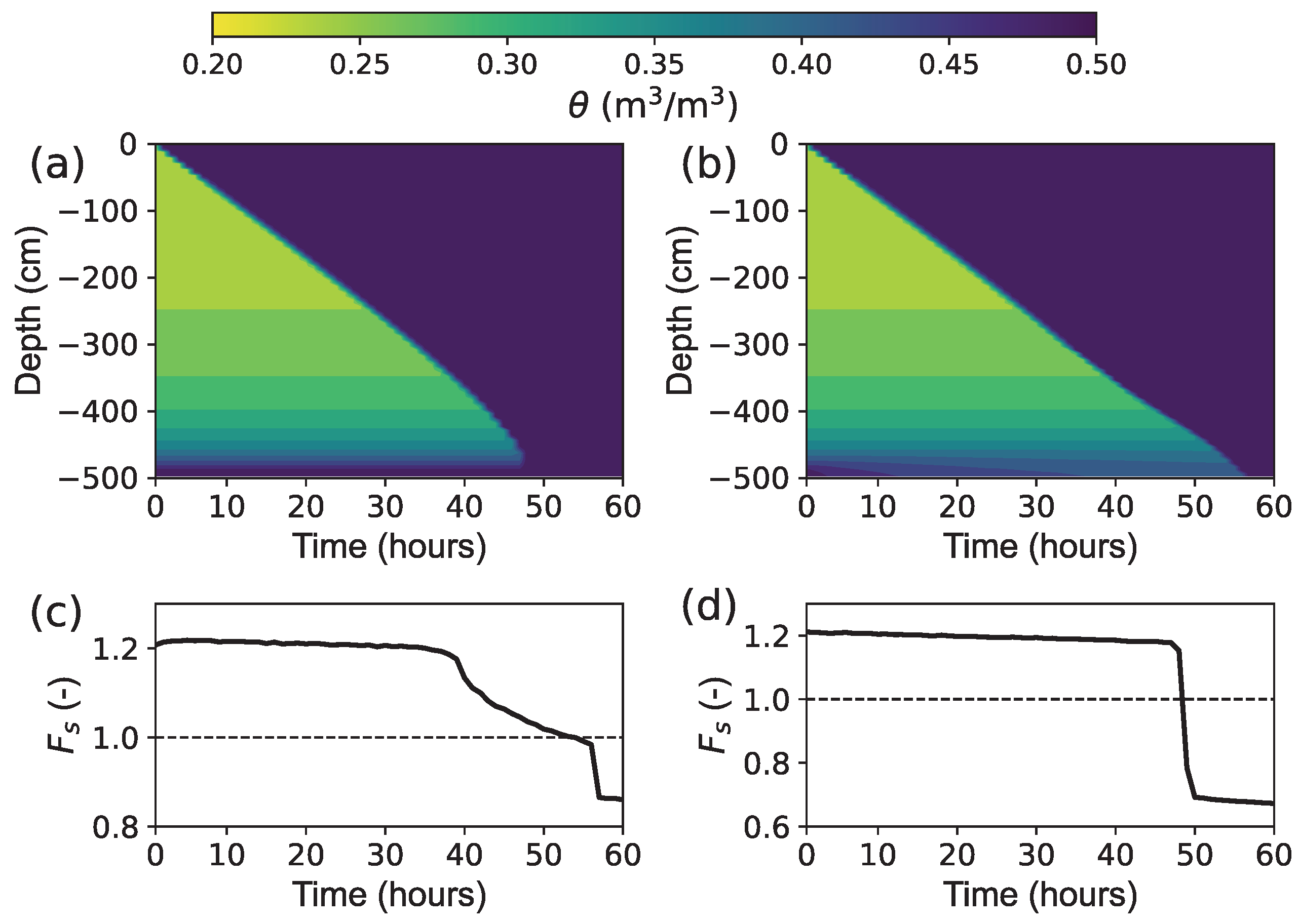
For slope stability, the F s in Case 7 exhibits a trend similar to Case 1 until approaching convergence (see Figure 12b). Around 50 h, F s in Case 7 declines sharply due to excess water accumulation and eventually converges to a steady state. In the later rainfall stages, F s in Case 7 falls substantially below that in the free-drainage scenario, with values consistently below 0.8 for deep-seated landslides, indicating a significantly more unstable slope condition. Additionally, the minimum F s was computed across all potential landslide geometries. Figure 13 presents two cases where we observed notable variations in minimum F s . In both cases, the soil water content progressed relatively uniformly until full saturation was reached. The minimum F s remained fairly stable prior to complete saturation of the upper soil layer, after which it began to change more significantly.

6. Discussion

6.1. Coupled Infiltration–Stability Model

Among various hydrological processes, soil infiltration plays a critical role in rainfall-induced landslides and constitutes a central component in developing coupled hydrological-geotechnical modeling frameworks [6]. The proposed coupled numerical model captures the essential vertical redistribution of pore water pressure under rainfall and is integrated into a 3D slope stability framework. Previous studies (e.g., [5,10,19]) have demonstrated that for many rainfall-induced landslides—particularly when slope materials are relatively homogeneous and rainfall infiltration dominates over subsurface lateral flow—the vertical infiltration assumption provides a reasonable approximation of the transient pore-pressure response. Thus, the combination of 1D infiltration modeling and 3D landslide geometry effectively balances computational accuracy with the complexity of real-world conditions. Furthermore, the use of a 3D model can mitigate the overly conservative tendencies of 1D models in most cases [22,55]. Previous work combining TRIGRS/GEOtop with Scoops3D can also simulate vertical soil profiles and three-dimensional slopes [55,56,57]. However, these studies generally pass outputs sequentially between models, reducing integration and complicating long-term maintenance and development. Moreover, Scoops3D uses a circular cross-section, which offers fewer degrees of freedom than the ellipsoidal cross-section examined here (defined by three axes). This ellipsoidal geometry provides greater flexibility for representing complex terrain, especially in shallow landslides. This approach enables efficient simulation of rainfall infiltration effects across complex three-dimensional geometries while preserving the essential hydromechanical coupling.
Compared with conceptual soil models such as the water tank (or reservoir) [23,58] approach and the commonly used one-dimensional infinite slope model [2,59], the proposed model more accurately captures key unsaturated flow dynamics and provides a more realistic, high-resolution assessment of potential failure surfaces from shallow to deep layers. Neglecting lateral flow introduces certain limitations, especially for highly anisotropic soils or topographically convergent slopes [60]. Nevertheless, the model developed in this study is designed with a flexible structure that facilitates future extensions. For lateral flow in space, only the potential gradients of the soil elements in the x and y directions need to be considered, which can be incorporated relatively easily from the 1D flow formulation. However, such an extension would substantially increase computational time [57], and the resulting performance gains might be limited. At the catchment scale in particular, the extent to which local improvements translate into global benefits remains uncertain and warrants further investigation [13].

6.2. Slope Stability Under Various Hydrological and Soil Layer Conditions

For rainfall intensities lower than K sat , increases in intensity lead to significant changes in shallow pore water pressure, consistent with predictions from most Richards-based models [25,61]. This behavior explains why the stability of shallow landslides begins to deteriorate at an early stage before reaching a steady state. The stability of deep landslides begins to decline at the onset of rainfall due to the changes in the stability of their shallow potential failure surfaces. This addresses a key limitation of the infinite slope model, which evaluates stability only at a fixed depth [55,62]. However, this phenomenon is not well represented by simplified physical models, such as the variable infiltration curve [13,58]. These models overlook unsaturated moisture migration within the soil, and focus solely on surface-to-subsurface water flux. As a result, increased rainfall intensity alters only average saturation, without capturing its spatial variability or interaction with complex slip surfaces. Moreover, heavy rainfall can result in surface ponding when the infiltration capacity of the soil is exceeded, thereby increasing soil weight and the associated sliding force. Prolonged surface–subsurface interactions could further raise the phreatic surface [63] and contribute to increased pore water pressure beneath the potential sliding surface, thereby heightening the risk of slope failure [64,65].
Lower initial soil moisture allows more rainfall to infiltrate deeply into the soil profile, potentially triggering deep-seated landslides. Due to stronger capillary forces under these conditions, changes in pore water pressure are relatively limited in the short term. However, prolonged rainfall can eventually lead to full saturation of deeper soil layers, resulting in delayed slope instability. In contrast, when initial soil moisture is relatively high, the soil capacity to store additional water is reduced, causing more rainfall to generate surface runoff. This promotes the rapid development of a potential slip surface and can lead to earlier slope failure. These findings support observed variations in failure mechanisms associated with initial soil moisture conditions—specifically, failure induced by the rise of a temporary perched water table in drier soils and by the advance of the wetting front in wetter soils [29]. Although, in theory, moisture redistribution from saturated deep soil to unsaturated shallow layers could occur via matric suction gradients, such upward migration is negligible under rainfall infiltration conditions, where gravity-driven flow dominates. Therefore, deep saturation tends to persist and continues to pose a significant landslide risk. However, this conclusion only applies to natural hillslopes, where soil moisture is influenced solely by hydrometeorological processes. For slopes within reservoir areas, reservoir operations directly interact with the groundwater in surrounding soils, thereby inducing transient alterations in hydrometeorological conditions that affect slope stability [66,67]. It is also worth noting that the relationship between initial hydrological conditions and landslide initiation is often nonlinear. Threshold effects may occur—for example, once soil moisture exceeds a certain level, the soil stability response to rainfall may intensify significantly. This provides essential information for assessing landslide early warning systems based on soil moisture [68,69,70]. The permeability of the underlying soil layer plays a pivotal role in governing slope hydrological response under rainfall. A low-permeability or impermeable layer beneath the slope may act as a hydraulic barrier, impeding downward infiltration and leading to the formation of a perched water table. This condition accelerates pore pressure build-up above the interface, which in turn reduces effective stress and promotes shallow or deep-seated failures. This confirms that horizontal drains are effective engineering measures, strategically placed to intercept perched water and enhance long-term slope resilience [71,72].

6.3. Limitations and Future Work

We adopted a fundamental numerical infiltration–stability modeling framework, assuming homogeneous surface conditions and simplified topography. While effective for capturing key mechanisms, it does not yet account for the spatial heterogeneity often present in real-world settings. Future work should incorporate complex terrain and variable hydrogeological properties to improve model applicability. Hardware-accelerated parallel computing can effectively enhance model performance and has the potential to further broaden its range of applications [73,74]. Additionally, including features such as macropore flow, root reinforcement, and evapotranspiration would extend the model to more realistic scenarios, such as cracked soils [75] or dynamic soil–vegetation–atmosphere interactions [76]. Further consideration of spatiotemporal rainfall patterns in numerical experiments would also provide significant research value. These extensions would enhance the model’s predictive capacity for natural slopes under diverse environmental conditions.

7. Conclusions

This study presents a numerical model that couples soil infiltration with 3D slope stability analysis to investigate rainfall-induced landslides. The model allows for the consideration of pore water pressure and stress distribution, which are necessary for 3D slope stability estimation. The model was validated against benchmark problems, and then utilized in numerical experiments to systematically explore the influence of various hydrological and geometric conditions on slope stability. The stability of shallow landslides is highly sensitive to rainfall intensity. For deep-seated landslides, intensity primarily affects the rate at which stability converges toward a constant value. Once rainfall intensity surpasses the soil saturated hydraulic conductivity, its additional impact on slope stability diminishes significantly. A high initial groundwater table is detrimental to slope stability, as it accelerates the weakening process, especially for deep landslides. Although upward moisture migration via matric suction gradients is theoretically possible, it is negligible during rainfall infiltration, where gravity-driven flow dominates. The permeability of the bottom boundary is a critical factor. Poor drainage efficiency leads to water accumulation and a sharp reduction in slope stability. The proposed model could potentially address limitations in existing hydrological-stability models, particularly those related to slope dimensionality, numerical computation, and complex hydrogeological boundary conditions that may occur under real-world conditions. Future research should focus on extending this model to incorporate more complex topographies and the spatial heterogeneity of soil hydrological properties.

Author Contributions

Conceptualization, G.C.; Methodology, G.C. and Y.L.; Software, G.C. and T.J.; Formal analysis, X.W. and L.H.; Investigation: G.C.; Resources, X.W. and L.H.; Data curation, Y.C. and T.J.; Writing-original draft, G.C. and T.J.; Writing—review & editing, T.J.; Visualization, L.H.; Supervision, X.W. and L.H.; Project administration, X.W.; Funding acquisition, G.C. and X.W. All authors have read and agreed to the published version of the manuscript.

Funding

This research was supported by Zhejiang Provincial Natural Science Foundation of China under Grant No. LQN25D010003 and Special Support Fund of Institutes of the Zhejiang Institute of Hydraulics and Estuary (ZIHEYS24002).

Data Availability Statement

The original contributions presented in the study are included in the article. Further inquiries can be directed to the corresponding author.

Conflicts of Interest

The authors declare no conflicts of interest.

References

  1. Alcántara-Ayala, I. Landslides in a changing world. Landslides 2025, 22, 2851–2865. [Google Scholar] [CrossRef]
  2. Zhang, K.; Xue, X.; Hong, Y.; Gourley, J.J.; Lu, N.; Wan, Z.; Hong, Z.; Wooten, R. iCRESTRIGRS: A coupled modeling system for cascading flood–landslide disaster forecasting. Hydrol. Earth Syst. Sci. 2016, 20, 5035–5048. [Google Scholar] [CrossRef]
  3. Marín-Rodríguez, N.J.; Vega, J.; Zanabria, O.B.; González-Ruiz, J.D.; Botero, S. Towards an understanding of landslide risk assessment and its economic losses: A scientometric analysis. Landslides 2024, 21, 1865–1881. [Google Scholar] [CrossRef]
  4. Sato, T.; Shuin, Y. Rainfall characteristics and magnitude control the volume of shallow and deep-seated landslides: Inferences from analyses using a simple runoff model. Geomorphology 2024, 466, 109453. [Google Scholar] [CrossRef]
  5. Lu, N.; Godt, J.W. Hillslope Hydrology and Stability; Cambridge University Press: Cambridge, UK, 2013. [Google Scholar]
  6. Bogaard, T.A.; Greco, R. Landslide hydrology: From hydrology to pore pressure. Wiley Interdiscip. Rev. Water 2016, 3, 439–459. [Google Scholar] [CrossRef]
  7. Greco, R.; Marino, P.; Bogaard, T.A. Recent advancements of landslide hydrology. Wiley Interdiscip. Rev. Water 2023, 10, e1675. [Google Scholar] [CrossRef]
  8. Rosso, R.; Rulli, M.C.; Vannucchi, G. A physically based model for the hydrologic control on shallow landsliding. Water Resour. Res. 2006, 42. [Google Scholar] [CrossRef]
  9. Godt, J.W.; Baum, R.L.; Lu, N. Landsliding in partially saturated materials. Geophys. Res. Lett. 2009, 36. [Google Scholar] [CrossRef]
  10. Baum, R.L.; Godt, J.W.; Savage, W.Z. Estimating the timing and location of shallow rainfall-induced landslides using a model for transient, unsaturated infiltration. J. Geophys. Res. Earth Surf. 2010, 115. [Google Scholar] [CrossRef]
  11. Montrasio, L.; Valentino, R. A model for triggering mechanisms of shallow landslides. Nat. Hazards Earth Syst. Sci. 2008, 8, 1149–1159. [Google Scholar] [CrossRef]
  12. Lu, N.; Şener-Kaya, B.; Wayllace, A.; Godt, J.W. Analysis of rainfall-induced slope instability using a field of local factor of safety. Water Resour. Res. 2012, 48. [Google Scholar] [CrossRef]
  13. Chen, G.; Zhang, K.; Wang, S.; Xia, Y.; Chao, L. iHydroSlide3D v1.0: An advanced hydrological–geotechnical model for hydrological simulation and three-dimensional landslide prediction. Geosci. Model Dev. 2023, 16, 2915–2937. [Google Scholar] [CrossRef]
  14. Liao, Z.; Hong, Y.; Wang, J.; Fukuoka, H.; Sassa, K.; Karnawati, D.; Fathani, F. Prototyping an experimental early warning system for rainfall-induced landslides in Indonesia using satellite remote sensing and geospatial datasets. Landslides 2010, 7, 317–324. [Google Scholar] [CrossRef]
  15. Chen, G.; Zhang, K.; Wang, S.; Chao, L. A prototype adaptive mesh generator for enhancing computational efficiency and accuracy in physically-based modeling of flood-landslide hazards. Environ. Model. Softw. 2025, 189, 106458. [Google Scholar] [CrossRef]
  16. Celia, M.A.; Bouloutas, E.T.; Zarba, R.L. A general mass-conservative numerical solution for the unsaturated flow equation. Water Resour. Res. 1990, 26, 1483–1496. [Google Scholar] [CrossRef]
  17. Srivastava, R.; Yeh, T.C.J. Analytical solutions for one-dimensional, transient infiltration toward the water table in homogeneous and layered soils. Water Resour. Res. 1991, 27, 753–762. [Google Scholar] [CrossRef]
  18. Yu, H.; Salgado, R.; Sloan, S.; Kim, J. Limit analysis versus limit equilibrium for slope stability. J. Geotech. Geoenviron. Eng. 1998, 124, 1–11. [Google Scholar] [CrossRef]
  19. Iverson, R.M. Landslide triggering by rain infiltration. Water Resour. Res. 2000, 36, 1897–1910. [Google Scholar] [CrossRef]
  20. Simoni, S.; Zanotti, F.; Bertoldi, G.; Rigon, R. Modelling the probability of occurrence of shallow landslides and channelized debris flows using GEOtop-FS. Hydrol. Processes Int. J. 2008, 22, 532–545. [Google Scholar] [CrossRef]
  21. Reid, M.E.; Christian, S.B.; Brien, D.L.; Henderson, S.T. Scoops3D: Software to Analyze 3D Slope Stability Throughout a Digital Landscape; Technical Report; US Geological Survey: Reston, VA, USA, 2015.
  22. Mergili, M.; Marchesini, I.; Rossi, M.; Guzzetti, F.; Fellin, W. Spatially distributed three-dimensional slope stability modelling in a raster GIS. Geomorphology 2014, 206, 178–195. [Google Scholar] [CrossRef]
  23. Aristizábal, E.; Vélez, J.I.; Martínez, H.E.; Jaboyedoff, M. SHIA_Landslide: A distributed conceptual and physically based model to forecast the temporal and spatial occurrence of shallow landslides triggered by rainfall in tropical and mountainous basins. Landslides 2016, 13, 497–517. [Google Scholar] [CrossRef]
  24. Brinkgreve, R.; Kumarswamy, S.; Swolfs, W.; Waterman, D.; Chesaru, A.; Bonnier, P.G.; Haxaire, A. PLAXIS 2016; PLAXIS bv: Delft, The Netherlands, 2016; pp. 1–16. [Google Scholar]
  25. Zhan, T.L.; Jia, G.; Chen, Y.M.; Fredlund, D.; Li, H. An analytical solution for rainfall infiltration into an unsaturated infinite slope and its application to slope stability analysis. Int. J. Numer. Anal. Methods Geomech. 2013, 37, 1737–1760. [Google Scholar] [CrossRef]
  26. Fan, L.; Lehmann, P.; Zheng, C.; Or, D. Rainfall intensity temporal patterns affect shallow landslide triggering and hazard evolution. Geophys. Res. Lett. 2020, 47, e2019GL085994. [Google Scholar] [CrossRef]
  27. Liu, X.; Wang, Y.; Leung, A.K. Numerical investigation of rainfall intensity and duration control of rainfall-induced landslide at a specific slope using slope case histories and actual rainfall records. Bull. Eng. Geol. Environ. 2023, 82, 333. [Google Scholar] [CrossRef]
  28. Oguz, E.A.; Depina, I.; Thakur, V. Effects of soil heterogeneity on susceptibility of shallow landslides. Landslides 2022, 19, 67–83. [Google Scholar] [CrossRef]
  29. Schilirò, L.; Poueme Djueyep, G.; Esposito, C.; Scarascia Mugnozza, G. The role of initial soil conditions in shallow landslide triggering: Insights from physically based approaches. Geofluids 2019, 2019, 2453786. [Google Scholar] [CrossRef]
  30. Richards, L.A. Capillary conduction of liquids through porous mediums. Physics 1931, 1, 318–333. [Google Scholar] [CrossRef]
  31. Mualem, Y. A new model for predicting the hydraulic conductivity of unsaturated porous media. Water Resour. Res. 1976, 12, 513–522. [Google Scholar] [CrossRef]
  32. Van Genuchten, M.T. A closed-form equation for predicting the hydraulic conductivity of unsaturated soils. Soil Sci. Soc. Am. J. 1980, 44, 892–898. [Google Scholar] [CrossRef]
  33. Vereecken, H.; Weynants, M.; Javaux, M.; Pachepsky, Y.; Schaap, M.; Genuchten, M.T.v. Using pedotransfer functions to estimate the van Genuchten–Mualem soil hydraulic properties: A review. Vadose Zone J. 2010, 9, 795–820. [Google Scholar] [CrossRef]
  34. Schaap, M.G.; Van Genuchten, M.T. A modified Mualem–van Genuchten formulation for improved description of the hydraulic conductivity near saturation. Vadose Zone J. 2006, 5, 27–34. [Google Scholar] [CrossRef]
  35. Vogel, T.; Van Genuchten, M.T.; Cislerova, M. Effect of the shape of the soil hydraulic functions near saturation on variably-saturated flow predictions. Adv. Water Resour. 2000, 24, 133–144. [Google Scholar] [CrossRef]
  36. Ippisch, O.; Vogel, H.J.; Bastian, P. Validity limits for the van Genuchten–Mualem model and implications for parameter estimation and numerical simulation. Adv. Water Resour. 2006, 29, 1780–1789. [Google Scholar] [CrossRef]
  37. van Dam, J.C.; Groenendijk, P.; Hendriks, R.F.; Kroes, J.G. Advances of modeling water flow in variably saturated soils with SWAP. Vadose Zone J. 2008, 7, 640–653. [Google Scholar] [CrossRef]
  38. Lu, N.; Likos, W.J. Suction stress characteristic curve for unsaturated soil. J. Geotech. Geoenviron. Eng. 2006, 132, 131–142. [Google Scholar] [CrossRef]
  39. Lu, N.; Godt, J.W.; Wu, D.T. A closed-form equation for effective stress in unsaturated soil. Water Resour. Res. 2010, 46. [Google Scholar] [CrossRef]
  40. Hovland, H.J. Three-dimensional slope stability analysis method. J. Geotech. Geoenviron. Eng. 1979, 105. [Google Scholar] [CrossRef]
  41. Xie, M.; Esaki, T.; Qiu, C.; Wang, C. Geographical Information System-Based Computational Implementation and Application of Spatial Three-Dimensional Slope Stability Analysis. Comput. Geotech. 2006, 33, 260–274. [Google Scholar] [CrossRef]
  42. Mergili, M.; Marchesini, I.; Alvioli, M.; Metz, M.; Schneider-Muntau, B.; Rossi, M.; Guzzetti, F. A Strategy for GIS-Based 3-D Slope Stability Modelling over Large Areas. Geosci. Model Dev. 2014, 7, 2969–2982. [Google Scholar] [CrossRef]
  43. Šimůnek, J.; Van Genuchten, M.T.; Šejna, M. The HYDRUS Software Package for Simulating Two- and Three-Dimensional Movement of Water, Heat, and Multiple Solutes in Variably-Saturated Media; Technical Manual, Version 1.0; PC Progress: Prague, Czech Republic, 2006; 241p. [Google Scholar]
  44. Wieder, W.; Boehnert, J.; Bonan, G.; Langseth, M. Regridded Harmonized World Soil Database v1.2. ORNL DAAC. 2014. Available online: https://ui.adsabs.harvard.edu/abs/2014ornl.data.1247W/abstract (accessed on 1 November 2025).
  45. Vanderborght, J.; Kasteel, R.; Herbst, M.; Javaux, M.; Thiéry, D.; Vanclooster, M.; Mouvet, C.; Vereecken, H. A set of analytical benchmarks to test numerical models of flow and transport in soils. Vadose Zone J. 2005, 4, 206–221. [Google Scholar] [CrossRef]
  46. Warrick, A.; Lomen, D.; Yates, S. A generalized solution to infiltration. Soil Sci. Soc. Am. J. 1985, 49, 34–38. [Google Scholar] [CrossRef]
  47. Li, Z.; Özgen-Xian, I.; Maina, F.Z. A mass-conservative predictor-corrector solution to the 1D Richards equation with adaptive time control. J. Hydrol. 2021, 592, 125809. [Google Scholar] [CrossRef]
  48. Phoon, K.K.; Tan, T.S.; Chong, P.C. Numerical simulation of Richards equation in partially saturated porous media: Under-relaxation and mass balance. Geotech. Geol. Eng. 2007, 25, 525–541. [Google Scholar] [CrossRef]
  49. Hungr, O.; Salgado, F.M.; Byrne, P. Evaluation of a three-dimensional method of slope stability analysis. Can. Geotech. J. 1989, 26, 679–686. [Google Scholar] [CrossRef]
  50. Gens, A.; Hutchinson, J.; Cavounidis, S. Three-dimensional analysis of slides in cohesive soils. Geotechnique 1988, 38, 1–23. [Google Scholar] [CrossRef]
  51. Lam, L.; Fredlund, D. A general limit equilibrium model for three-dimensional slope stability analysis. Can. Geotech. J. 1993, 30, 905–919. [Google Scholar] [CrossRef]
  52. Tozato, K.; Dolojan, N.L.J.; Touge, Y.; Kure, S.; Moriguchi, S.; Kawagoe, S.; Kazama, S.; Terada, K. Limit equilibrium method-based 3D slope stability analysis for wide area considering influence of rainfall. Eng. Geol. 2022, 308, 106808. [Google Scholar] [CrossRef]
  53. An, H.; Viet, T.T.; Lee, G.; Kim, Y.; Kim, M.; Noh, S.; Noh, J. Development of time-variant landslide-prediction software considering three-dimensional subsurface unsaturated flow. Environ. Model. Softw. 2016, 85, 172–183. [Google Scholar] [CrossRef]
  54. Park, D.W.; Nikhil, N.V.; Lee, S.R. Landslide and Debris Flow Susceptibility Zonation Using TRIGRS for the 2011 Seoul Landslide Event. Nat. Hazards Earth Syst. Sci. 2013, 13, 2833–2849. [Google Scholar] [CrossRef]
  55. Tran, T.V.; Alvioli, M.; Lee, G.; An, H.U. Three-dimensional, time-dependent modeling of rainfall-induced landslides over a digital landscape: A case study. Landslides 2018, 15, 1071–1084. [Google Scholar] [CrossRef]
  56. He, J.; Qiu, H.; Qu, F.; Hu, S.; Yang, D.; Shen, Y.; Zhang, Y.; Sun, H.; Cao, M. Prediction of spatiotemporal stability and rainfall threshold of shallow landslides using the TRIGRS and Scoops3D models. Catena 2021, 197, 104999. [Google Scholar] [CrossRef]
  57. Rangarajan, S.; Rahardjo, H.; Satyanaga, A.; Li, Y. Influence of 3D subsurface flow on slope stability for unsaturated soils. Eng. Geol. 2024, 339, 107665. [Google Scholar] [CrossRef]
  58. He, X.; Hong, Y.; Vergara, H.; Zhang, K.; Kirstetter, P.E.; Gourley, J.J.; Zhang, Y.; Qiao, G.; Liu, C. Development of a coupled hydrological-geotechnical framework for rainfall-induced landslides prediction. J. Hydrol. 2016, 543, 395–405. [Google Scholar] [CrossRef]
  59. Cui, H.; Ji, J.; Hürlimann, M.; Medina, V. Probabilistic and physically-based modelling of rainfall-induced landslide susceptibility using integrated GIS-FORM algorithm. Landslides 2024, 21, 1461–1481. [Google Scholar] [CrossRef]
  60. Kim, J.; Mohanty, B.P. Influence of lateral subsurface flow and connectivity on soil water storage in land surface modeling. J. Geophys. Res. Atmos. 2016, 121, 704–721. [Google Scholar] [CrossRef]
  61. Pham, K.; Kim, D.; Choi, H.J.; Lee, I.M.; Choi, H. A numerical framework for infinite slope stability analysis under transient unsaturated seepage conditions. Eng. Geol. 2018, 243, 36–49. [Google Scholar] [CrossRef]
  62. Milledge, D.; Griffiths, D.; Lane, S.; Warburton, J. Limits on the validity of infinite length assumptions for modelling shallow landslides. Earth Surf. Process. Landf. 2012, 37, 1158–1166. [Google Scholar] [CrossRef]
  63. Wang, J.; Wang, Z.; Sun, G. Phreatic surface calculation and stability analysis of three-dimensional slopes under rainfall infiltration. Bull. Eng. Geol. Environ. 2024, 83, 51. [Google Scholar] [CrossRef]
  64. Wasowski, J.; Lamanna, C.; Gigante, G.; Casarano, D. High resolution satellite imagery analysis for inferring surface–subsurface water relationships in unstable slopes. Remote Sens. Environ. 2012, 124, 135–148. [Google Scholar] [CrossRef]
  65. Ye, X.; Zhu, H.H.; Wang, J.; Zhang, Q.; Shi, B.; Schenato, L.; Pasuto, A. Subsurface multi-physical monitoring of a reservoir landslide with the fiber-optic nerve system. Geophys. Res. Lett. 2022, 49, e2022GL098211. [Google Scholar] [CrossRef]
  66. Xia, M.; Ren, G.M.; Zhu, S.S.; Ma, X.L. Relationship between landslide stability and reservoir water level variation. Bull. Eng. Geol. Environ. 2015, 74, 909–917. [Google Scholar] [CrossRef]
  67. Kafle, L.; Xu, W.J.; Zeng, S.Y.; Nagel, T. A numerical investigation of slope stability influenced by the combined effects of reservoir water level fluctuations and precipitation: A case study of the Bianjiazhai landslide in China. Eng. Geol. 2022, 297, 106508. [Google Scholar] [CrossRef]
  68. Wicki, A.; Lehmann, P.; Hauck, C.; Seneviratne, S.I.; Waldner, P.; Stähli, M. Assessing the potential of soil moisture measurements for regional landslide early warning. Landslides 2020, 17, 1881–1896. [Google Scholar] [CrossRef]
  69. Marino, P.; Peres, D.J.; Cancelliere, A.; Greco, R.; Bogaard, T.A. Soil moisture information can improve shallow landslide forecasting using the hydrometeorological threshold approach. Landslides 2020, 17, 2041–2054. [Google Scholar] [CrossRef]
  70. Abraham, M.T.; Satyam, N.; Rosi, A.; Pradhan, B.; Segoni, S. Usage of antecedent soil moisture for improving the performance of rainfall thresholds for landslide early warning. CATENA 2021, 200, 105147. [Google Scholar] [CrossRef]
  71. Rahardjo, H.; Hritzuk, K.; Leong, E.; Rezaur, R. Effectiveness of horizontal drains for slope stability. Eng. Geol. 2003, 69, 295–308. [Google Scholar] [CrossRef]
  72. Sun, H.y.; Ge, Q.; Yu, Y.; Shuai, F.x.; Lü, C.c. A new self-starting drainage method for slope stabilization and its application. Bull. Eng. Geol. Environ. 2021, 80, 251–265. [Google Scholar] [CrossRef]
  73. Alvioli, M.; Baum, R.L. Parallelization of the TRIGRS model for rainfall-induced landslides using the message passing interface. Environ. Model. Softw. 2016, 81, 122–135. [Google Scholar] [CrossRef]
  74. Chen, G.; Zhang, K.; Wang, S.; Jia, T. PHyL v1.0: A parallel, flexible, and advanced software for hydrological and slope stability modeling at a regional scale. Environ. Model. Softw. 2024, 172, 105882. [Google Scholar] [CrossRef]
  75. Luo, Y.; Hou, X.; Zhang, J.; Wang, Y.; Hu, M.; Jiang, G.; Tang, C.S. Exploring the effects of weather-driven dynamics of desiccation cracks on hydrological process of expansive clay slope: Insights from physical model test. J. Hydrol. 2025, 656, 133011. [Google Scholar] [CrossRef]
  76. Zhang, B.; Tian, L.; He, C.; He, X. Response of erosive precipitation to vegetation restoration and its effect on soil and water conservation over China’s Loess Plateau. Water Resour. Res. 2023, 59, e2022WR033382. [Google Scholar] [CrossRef]
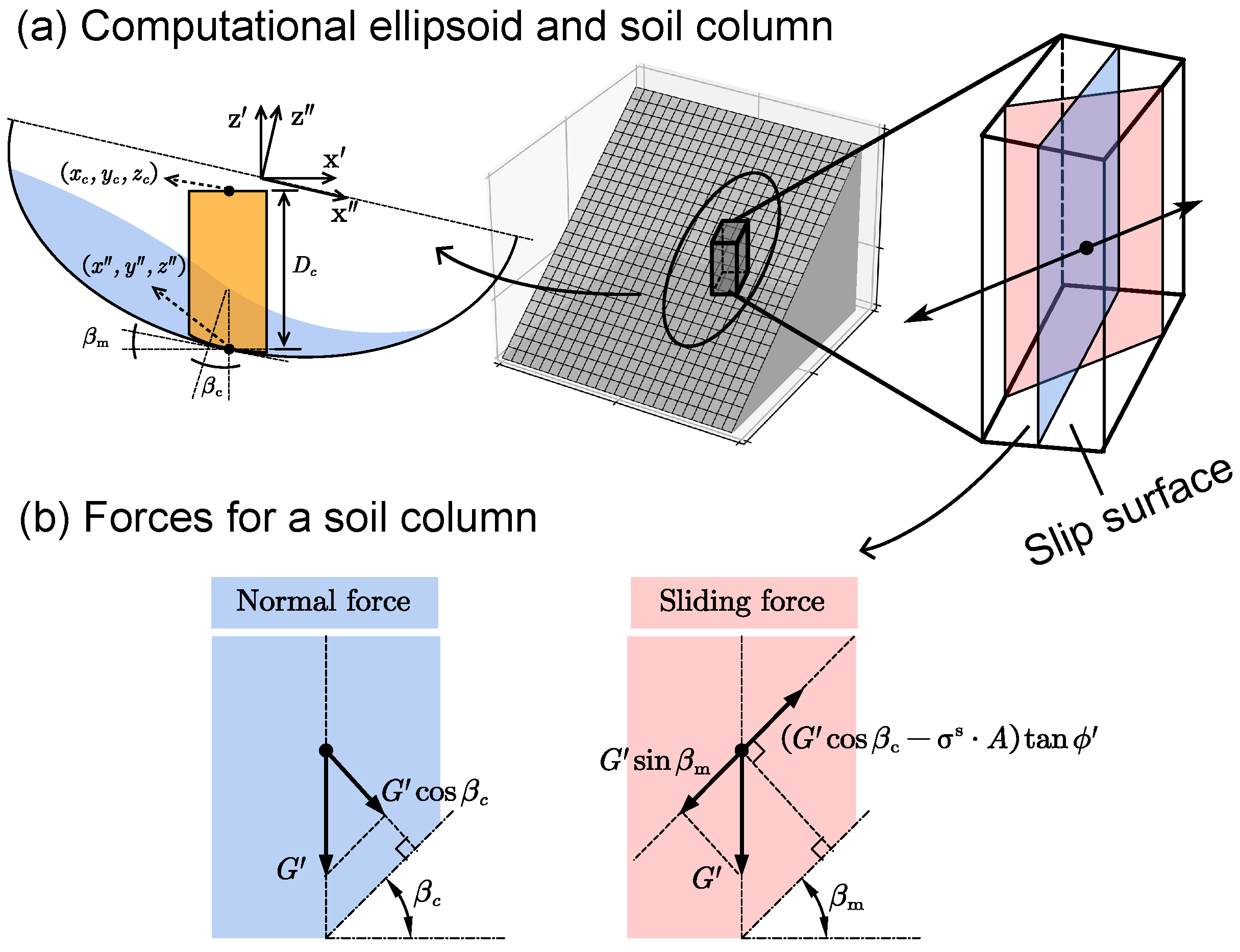
Figure 1. Theoretical framework of 3D slope stability model: (a) features of a potential failure under a longitudinal section; (b) forces acting at a soil column.
Water 17 03316 g001
Figure 2. Benchmarking problems of (a) infiltration in layered soils and (b) slope stability of a spherical sliding surface.
Water 17 03316 g002
Figure 3. Comparison between numerical and analytical solutions of soil-water pressure head profiles under a steady rainfall rate of q a = 0.5 cm · d 1 for layered soils: (a) loam-sand; (b) sand-loam; (c) clay-sand.
Water 17 03316 g003
Figure 4. Simulation results (water content profiles) of Warrick’s problem against the analytical solution.
Water 17 03316 g004
Figure 5. (a) Comparison between 3D and 1D (infinite) slope failure scenarios on an inclined slope, illustrating various sliding surfaces from shallow to deep failures. (b) Comparison of calculated slope stability results—factor of safety ( F s )—between the 3D and 1D models, corresponding to the failure depths shown in (a).
Water 17 03316 g005
Figure 6. (a) SWCC for typical soils, (b) SSCC for typical soils in terms of the effective degree of saturation, (c) SSCC for the typical soils in terms of matric suction, and (d) factor of safety for typical soils in terms of the effective degree of saturation.
Water 17 03316 g006
Figure 7. (a) Fitted volumetric water content versus observations; (b) soil hydraulic conductivity as a function of pressure head.
Water 17 03316 g007
Figure 8. Simulated results for Case 1, Case 2, and Case 3. (a) Pressure head profiles in Case 1; (b) factor of safety in Case 1; (c) pressure head profiles in Case 2; (d) factor of safety in Case 2; (e) pressure head profiles in Case 3; (f) factor of safety in Case 3.
Water 17 03316 g008
Figure 9. Simulated results for Case 4. (a) Pressure head profiles; (b) factor of safety.
Water 17 03316 g009
Figure 10. Simulated results for Case 5. (a) Pressure head profiles; (b) factor of safety.
Water 17 03316 g010
Figure 11. Simulated results for Case 6. (a) Pressure head profiles; (b) factor of safety.
Water 17 03316 g011
Figure 12. Simulated results for Case 7. (a) Pressure head profiles; (b) factor of safety.
Water 17 03316 g012
Figure 13. Time–depth distribution of soil water content for (a) Case 6 and (b) Case 7, with corresponding factor of safety shown in (c) and (d), respectively. The factor of safety represents the minimum value among all potential landslide geometries.
Water 17 03316 g013
Table 1. Soil parameters used for benchmark validation simulations.
Soil θ r θ s α ( cm 1 )n K sat ( cm · d 1 ) c s (kPa) ϕ ( ) n p γ s ( kN / m 3 )
Sand0.0450.430.153.010005400.4321
Loam0.0800.430.041.6501022.50.4313
Clay0.1000.400.011.1104019.50.4719.5
Table 2. Comparison of computed safety factors for a typical slope with values reported in previous studies.
Reference F s
Hungr et al. [49]1.422
Gens et al. [50]1.41
Lam and Fredlund [51]1.386∼1.472
Xie et al. [41]1.443
Mergili et al. [42]1.38
Tozato et al. [52]1.392
Reid et al. [21] (Scoops3D)1.400
This work1.408
Table 3. Soil parameters for numerical experiments.
θ r θ s α ( cm 1 )n K sat ( cm · d 1 ) λ c s (kPa) ϕ (°) γ s ( kN / m 3 )
0.180.500.051.6112.320.510.1729.6318.38
Table 4. Numerical experiments setup.
CaseVertical Depth (cm)Soil TypeInitial ConditionBottom BoundaryRainfall
1500S1 GWL = 500 cmFree drainage0.5 K sat
2500S1 GWL = 500 cmFree drainage1.0 K sat
3500S1 GWL = 500 cmFree drainage1.5 K sat
4500S1 GWL = 400 cmFree drainage0.5 K sat
5500S1 GWL = 300 cmFree drainage0.5 K sat
6300 + 200S1 + S2 GWL = 500 cmFree drainage0.5 K sat
7500S1 GWL = 500 cmZero flux0.5 K sat
Disclaimer/Publisher’s Note: The statements, opinions and data contained in all publications are solely those of the individual author(s) and contributor(s) and not of MDPI and/or the editor(s). MDPI and/or the editor(s) disclaim responsibility for any injury to people or property resulting from any ideas, methods, instructions or products referred to in the content.