Article

High-Resolution Spatiotemporal Mapping of Surface Soil Moisture Using ConvLSTM Model and Sentinel-1 Data

Department of Civil and Environmental Engineering, Morgan State University, Baltimore, MD 21251, USA
*
Author to whom correspondence should be addressed.
Water 2025, 17(22), 3300; https://doi.org/10.3390/w17223300
Submission received: 17 October 2025 / Revised: 11 November 2025 / Accepted: 12 November 2025 / Published: 18 November 2025
(This article belongs to the Section Soil and Water)

Abstract

Soil moisture plays a crucial role in hydrological processes and serves as a key driver of rainfall-induced landslides, especially in regions with steep terrain and intense precipitation. Traditional landslide risk models often oversimplify soil moisture and infiltration dynamics, which limits their predictive accuracy. This study presents a deep learning-based framework for generating high-resolution, spatiotemporal Surface Soil Moisture (SSM) maps for Prince George’s County, Maryland—a region highly susceptible to rainfall-triggered landslides—aimed at improving infiltration modeling and landslide prediction. A Convolutional Long Short-Term Memory (ConvLSTM) network integrates static spatial features (elevation, slope, soil type) with multi-temporal meteorological variables (precipitation, temperature, humidity, wind speed, evapotranspiration) and vegetation indices. The model is trained using dense SSM maps derived from Sentinel-1 SAR data processed through a change detection algorithm, providing a physically meaningful alternative to sparse in-situ observations. To address data imbalance, a two-pass patch extraction strategy was implemented to enhance representation of high-SSM conditions. The framework leverages high-performance computing resources to process large-scale, multi-temporal raster datasets efficiently. Evaluation results show strong predictive performance, with the two-day model achieving R 2 = 0.72, correlation = 0.85, RMSE = 0.154, and MAE = 0.103. The results demonstrate the model’s capability to produce fine-resolution, wall-to-wall SSM maps that capture the spatial and temporal dynamics of surface soil moisture, supporting the development of early warning systems and landslide hazard mitigation strategies.

1. Introduction

Surface Soil Moisture (SSM) is a critical component of the hydrological cycle, influencing agricultural productivity, weather forecasting, and natural hazard mitigation. In particular, it plays a pivotal role in landslide initiation by controlling pore water pressure and reducing effective stress along potential failure surfaces [1,2,3,4,5]. Rainfall-triggered landslides pose serious threats to human life, infrastructure, and ecosystems, especially in regions with steep slopes and high precipitation intensity [6,7,8,9,10,11,12,13]. As such, accurate and spatially explicit SSM data are indispensable for effective landslide hazard assessment and early warning systems [14,15,16,17,18,19,20].
Rainfall is one of the main causes of rainfall-induced landslides, which are common types of slope failures [21]. However, many previous studies have used simplified assumptions about how rainfall translates into SSM and infiltration. Some studies assume that all rainfall infiltrates or that a fixed percentage can represent infiltration, without considering factors such as slope angle, soil type, or surface conditions [22]. These simplifications often cause large errors, especially in regions with heavy rainfall, because actual infiltration is usually much lower than total rainfall [23]. Therefore, advanced modeling approaches are needed to better simulate SSM and infiltration from rainfall and more accurately assess their role in triggering landslides.
An advanced method for accurately representing SSM and infiltration processes is the use of physical models that simulate the complex interactions between surface and subsurface water flow [24,25,26,27,28]. Although these physical models can capture hydrological processes across saturated and unsaturated zones, they come with significant limitations due to high computational demands and extensive calibration requirements, making them case-specific and difficult to generalize across regions.
To overcome these challenges and enhance spatially explicit SSM estimation for slope-stability analysis, data-driven approaches have gained increasing attention. Recent advances in Machine Learning (ML) offer a promising pathway for high-resolution SSM mapping. Unlike physical models, ML techniques can rapidly adapt to different environments by analyzing historical data patterns, allowing for broader applicability and improved predictive accuracy without being constrained by case-specific physical assumptions. The efficiency, scalability, and adaptability of ML models make them a strong complement to or replacement for traditional physical models in infiltration studies. Several studies have demonstrated the use of ML algorithms—such as Random Forests, Support Vector Machines, and Artificial Neural Networks—to predict soil moisture using weather, vegetation, and soil data [29,30,31,32]. SSM is influenced by a complex interplay of spatial and temporal factors, including precipitation patterns, land surface temperature, evapotranspiration, wind, vegetation dynamics, and soil properties. Capturing these dependencies requires models that can process sequences of spatial data over time [33,34]. Although numerous studies have investigated the spatiotemporal dynamics of SSM, a common limitation is their reliance on sparse, point-based observations from networks such as SCAN (Soil Climate Analysis Network) or ISMN (International Soil Moisture Network), rather than spatially continuous datasets that are critical for large-scale environmental modeling and prediction. In particular, many studies (e.g., [35,36,37,38,39]) have applied ML techniques to estimate soil moisture at individual locations using meteorological inputs, without producing high-resolution, spatially continuous maps. This restricts the applicability of such models in domains such as hydrology and geohazard assessment—especially for landslide prediction—where accurate wall-to-wall SSM mapping at high spatial and temporal resolution is essential.
One of the primary challenges in addressing this gap lies in the computational demands associated with processing full-resolution raster datasets over hundreds of time steps and multiple input variables. Traditional ML workflows, which typically rely on loading entire rasters into memory, are not scalable for such large datasets. To address this limitation, the present study proposes an optimized deep learning architecture for spatiotemporal SSM modeling. The model is trained using high-performance computing resources, allowing efficient processing of large-scale, multi-temporal raster inputs and generation of high-resolution SSM maps suitable for downstream geohazard applications.
On the other hand, both traditional methods of SSM monitoring and supervised ML models typically rely on in-situ sensors and gravimetric sampling as sources of observation and ground-truth labels to ensure predictive reliability. While these methods provide high accuracy in a specific location, they suffer from limited spatial coverage and are prohibitively expensive to implement over large areas [40]. This spatial sparsity can lead to overfitting to particular sites and reduce the generalizability of models across diverse landscapes. Satellite remote sensing offers broader spatial coverage through missions such as SMAP, SMOS, and ASCAT [41,42]. However, the coarse spatial resolution of these products (typically 10–36 km) limits their applicability in localized studies, such as landslide risk assessment, which demands fine-scale soil moisture data.
Although various downscaling techniques have been developed to improve spatial resolution using ancillary datasets—such as the approach proposed by Liu et al. [43]—their effectiveness often remains inconsistent, particularly in heterogeneous or topographically complex environments. This study overcomes these challenges by employing Sentinel-1 backscatter data processed using a change detection model, which generates dense, high-resolution, and self-calibrated SSM maps.
To address these challenges and bridge the current gaps in SSM modeling, this study presents a novel deep learning framework for producing high-resolution spatiotemporal SSM maps. The proposed approach leverages a Convolutional Long Short-Term Memory (ConvLSTM) network to effectively learn from a combination of static variables (e.g., elevation, slope, soil texture), multi-temporal meteorological data (e.g., precipitation, temperature, wind speed, humidity, evapotranspiration) and temporal vegetation coverage. By training on dense, high-resolution Sentinel-1-derived SSM labels obtained via a self-calibrated change detection model, this study bypasses the limitations of sparse in-situ data while ensuring physically meaningful predictions. This integration of Sentinel-1-derived SSM with the ConvLSTM model represents a novel approach that addresses the aforementioned challenges and enables continuous, high-resolution SSM prediction in both space and time, rather than relying on point-based estimates. The resulting satellite–ML framework provides a vital tool for infiltration modeling, hydrological forecasting, and landslide risk assessment—particularly in data-scarce and topographically heterogeneous regions.

2. Materials and Methods

2.1. Study Area

Prince George County, located in central Maryland, serves as an ideal case study area due to its geographic diversity, varied topography, and susceptibility to extreme weather events such as heavy rainfall and landslides. The county was selected to develop and validate the ML model on a smaller scale, with plans to later extend the framework to the broader Maryland region or other states. Covering about 500 square miles, Prince George County includes a mix of urban, suburban, and rural areas, representing the land use and environmental diversity of the Mid-Atlantic region.
Geologically, the county lies within the transition zone between the Atlantic Coastal Plain and the Piedmont Plateau, resulting in complex terrain, varying slope gradients, and soil types that influence hydrological and slope stability dynamics. The climate is humid subtropical with year-round precipitation, providing suitable conditions for modeling rainfall-induced processes such as SSM variability and slope failures. Significantly, according to the most recent landslide inventories compiled by the Maryland Department of Transportation (MDOT)-State Highway Administration (SHA), the United States Geological Survey (USGS), and National Aeronautics and Space Administration (NASA), Maryland experienced 129 recorded landslides between 2008 and 2019, with the majority classified as shallow failures (Figure 1).
As shown in Figure 2a, Prince George County has experienced the highest number of landslide events in Maryland, accounting for approximately 30% of the state’s recorded occurrences. Given that this county is also one of the most densely populated in Maryland, evaluating, forecasting, and mitigating landslide hazards is critical for protecting both communities and infrastructure.
Figure 2b further highlights a strong temporal correlation between rainfall and landslide frequency, with peak events occurring in 2011, 2014, and 2018—years that also recorded the highest annual precipitation. This pattern underscores the significant role of rainfall and subsequent infiltration as primary triggering factors for landslides in the region.
In addition, Figure 2c,d illustrates the relationship between the number of landslide events and both rainfall intensity and SSM levels. The data indicates that many landslides were triggered by relatively low rainfall amounts, suggesting that certain high-risk slopes in Maryland are susceptible even to minor precipitation events. Conversely, a more pronounced trend is observed between landslide occurrence and increased SSM, highlighting the importance of subsurface hydrological conditions in slope failure. This finding reinforces the need to model and monitor SSM dynamics rather than relying solely on direct rainfall as a predictive variable.
This study aims to investigate these relationships in more depth to predict SSM by rainfall for use in future landslide studies, using Prince George County as a representative and data-rich case study area. The region’s exposure to climate-related hazards, ongoing urban development, and stormwater management challenges further justify its selection as a critical focus for developing advanced models for the prediction of landslides.

2.2. Data Preparation

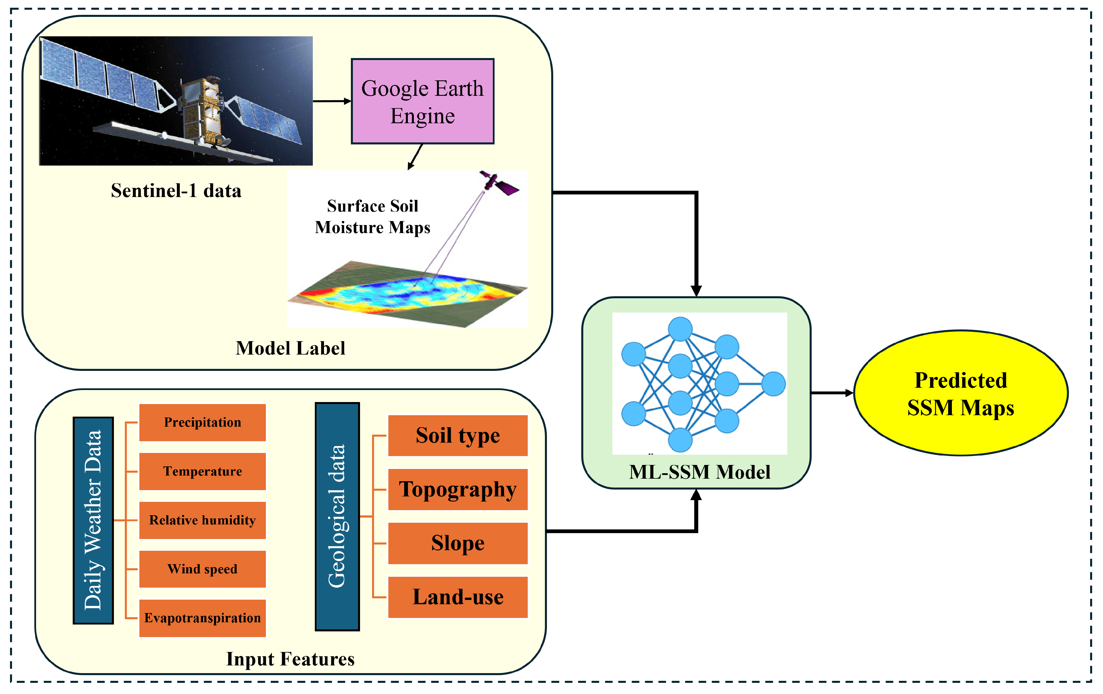
Figure 3 presents the workflow to develop a ML-based Surface Soil Moisture model (ML-SSM), utilizing SSM maps derived from Sentinel-1 satellite data. As shown in the diagram, various datasets are required to build and train the ML-SSM model, including the target variable (SSM), weather parameters, and geological characteristics. These inputs consist of spatial-temporal data, such as SSM maps, weather variables maps, land use/land cover maps, and spatially static data, such as soil type, topography, and slope maps.

2.2.1. Sentinel-1 Data to Generate SSM Maps

The target data used to evaluate the ML-SSM model consist of SSM maps generated from Sentinel-1 imagery at six-day intervals. Sentinel-1, a component of the European Space Agency’s Copernicus Program, has provided high-resolution, radar-based observations since 2014. Its C-band Synthetic Aperture Radar (SAR) sensor enables continuous data acquisition under all weather and lighting conditions [44], making it highly suitable for SSM monitoring. With two satellites, Sentinel-1A and Sentinel-1B, operating on a 12-day repeat cycle, the combination of their datasets effectively results in a six-day revisit period [45]. This frequent update cycle facilitates the generation of SSM maps every six days, supporting applications such as large-scale hydrological research and landslide hazard assessment. Sentinel-1’s Interferometric Wide (IW) mode, covering a 250 km swath at a resolution of 20 m × 22 m, ensures the precise detection of subtle surface variations [46]. In this study, SSM estimates were derived using signals recorded in vertical-vertical (VV) polarization mode, and the final maps were produced at a spatial resolution of 15 m.

2.2.2. Weather Data

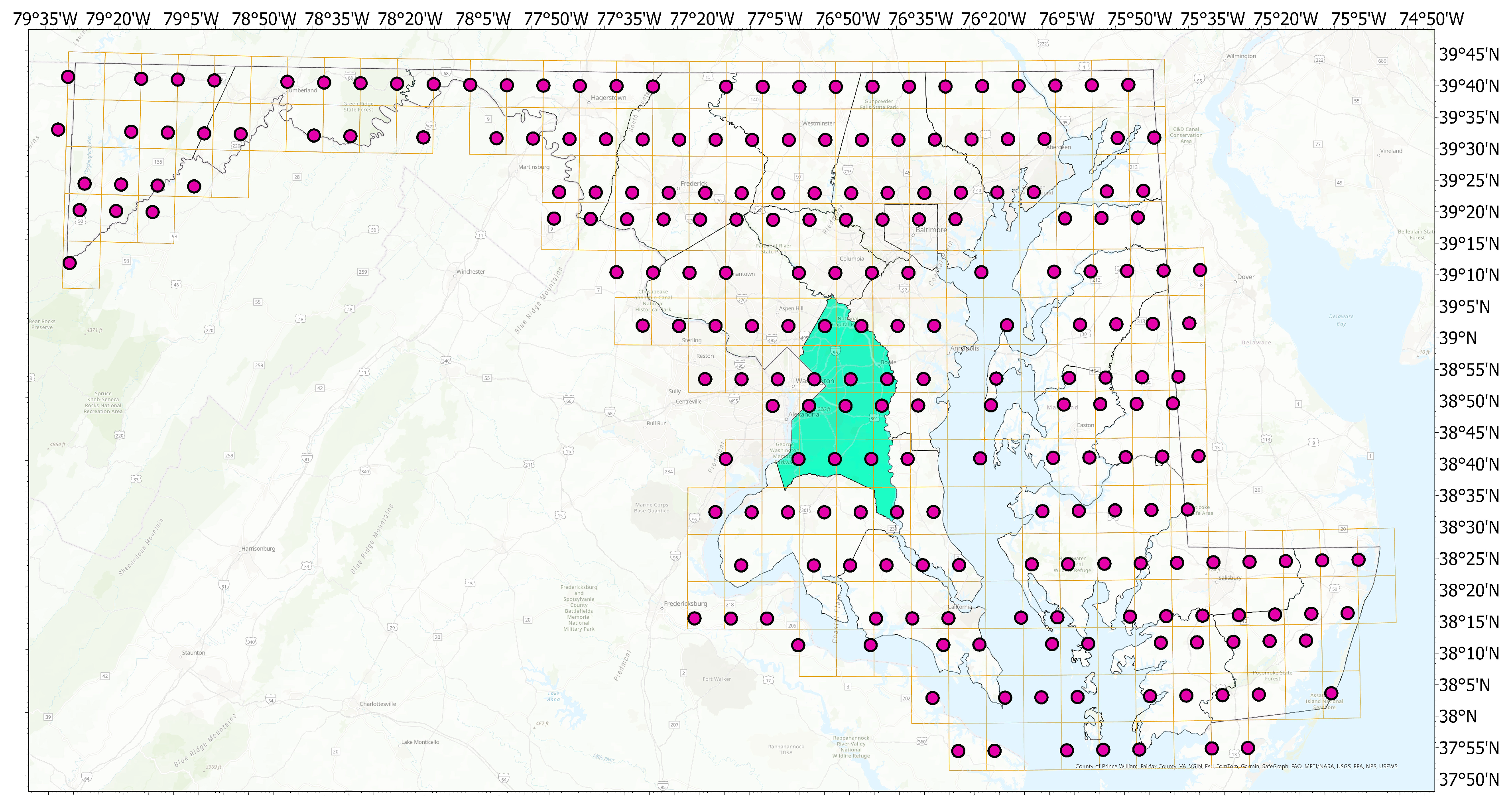
To develop the ML-SSM model, it is essential to compile a time series of daily climate variables, including precipitation, maximum and minimum temperature, relative humidity, wind speed, and evapotranspiration (ET). These datasets were obtained from the Open-Meteo database at a spatial resolution of 9 km. However, this resolution is too coarse for high-resolution spatial modeling; therefore, the datasets were interpolated and resampled to produce weather variable maps at a 15-m resolution. In this study, the Inverse Distance Weighting (IDW) method was applied to interpolate all weather variables. The IDW method is widely used and accepted for interpolating meteorological variables such as precipitation and temperature, particularly when measurement points are limited and sparsely distributed, and when spatial variation is relatively smooth [47]. The locations of the original weather data points used for interpolation are shown in Figure 4.
The final SSM observations derived from Sentinel-1 were available only at 12-day intervals (although nominally every 6 days, missing data led to using a 12-day interval). This data gap introduces some limitations in temporal consistency. To address this challenge during ML model training, the meteorological data were aligned with the available observation dates and prepared in three configurations to capture all possible temporal relationships between the weather variables and the target SSM values. The 1-day model used weather variables from the exact observation date. The 2-day model used cumulative rainfall and evapotranspiration, and averaged other variables, over the observation date and the preceding day. The 3-day model extended this to the observation date and the two preceding days. These three datasets allowed comparison of how different temporal representations of meteorological conditions affected prediction performance.
  • 1-day model: exact date values.
  • 2-day model: observation date + 1 day before.
  • 3-day model: observation date + 2 days before.

2.2.3. Geological Data

To prepare the static maps, a detailed soil map was obtained from the Maryland Soil Survey Geographic Database (SSURGO). Soil polygons located along highways that lacked attribute information on soil properties and materials were identified, and the percentages of clay, silt, and sand for these polygons were estimated using the average values from neighboring polygons. In parallel, topographic features were extracted using 1/3 arc-second LiDAR-based Digital Elevation Models (DEMs) specific to Maryland. Subsequently, the slope map was derived from the DEM using ArcGIS Pro 3.3.0 tools. To monitor vegetation dynamics over time, Normalized Difference Vegetation Index (NDVI) maps were generated using Sentinel-2 satellite imagery within the Google Earth Engine (GEE) platform.
Sentinel-2, part of the Copernicus program by the European Space Agency (ESA), provides high-resolution optical imagery with a spatial resolution of up to 10 m and a revisit time of 5 days, making it particularly suitable for vegetation analysis [48]. NDVI was calculated using the standard formula:
NDVI = NIR RED NIR + RED
where NIR and RED correspond to reflectance values from the near-infrared (Band 8) and red (Band 4) wavelengths, respectively.
In GEE platform, Sentinel-2 surface reflectance data were pre-processed to mask clouds using the QA60 band and a cloud probability threshold. NDVI was then computed for each image and temporally aggregated to generate consistent NDVI maps that match the acquisition dates of the SSM maps. These NDVI maps provide valuable information of vegetation cover, which is an essential parameter that influences SSM and rainfall infiltration [49].
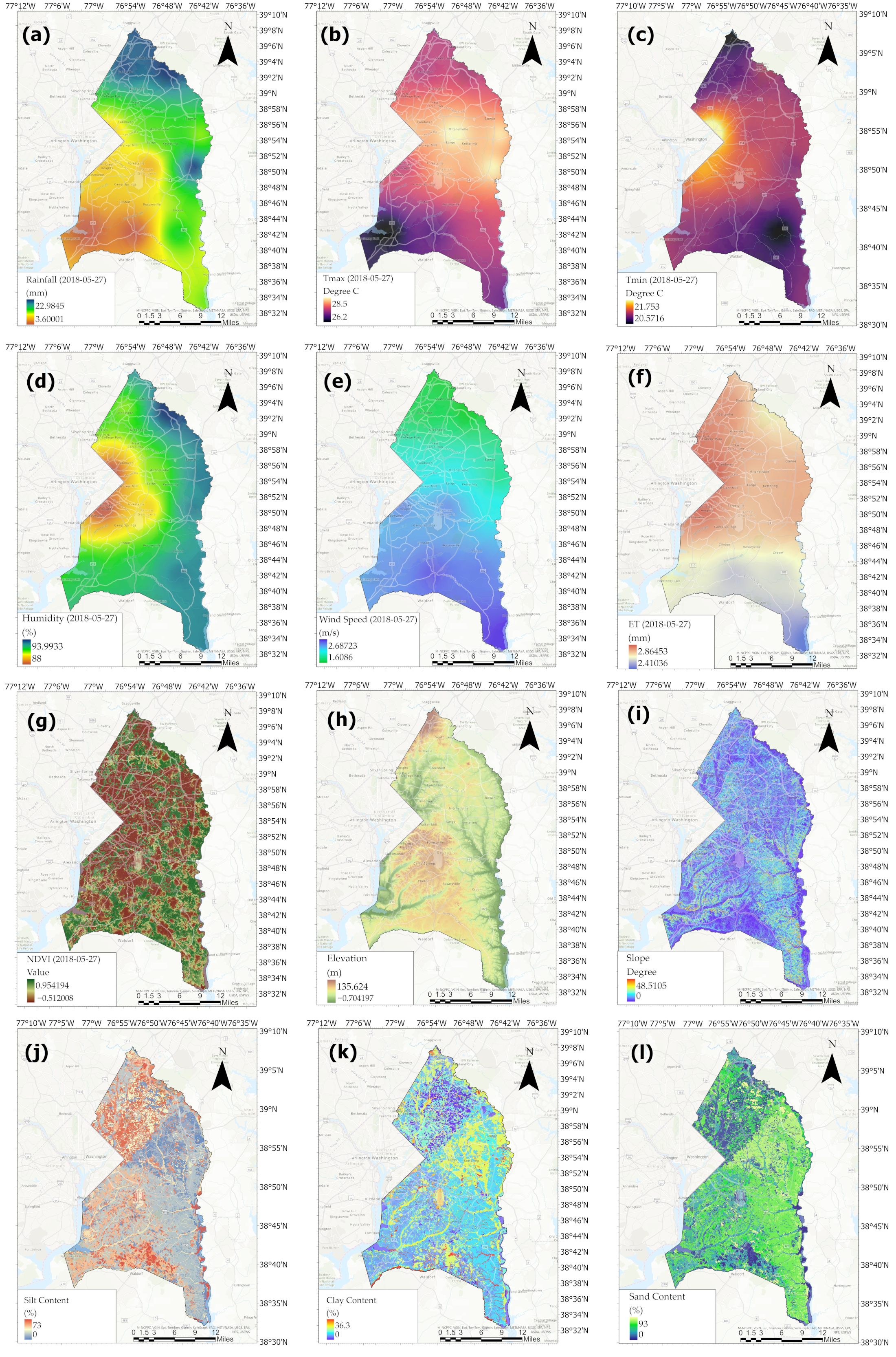
Figure 5 illustrates the spatial distribution of all input parameters used to develop the ML-SSM model for the study area. The figure includes representative maps for 27 May 2018, showing spatiotemporal variables such as rainfall, maximum and minimum temperature, humidity, wind speed, ET, and NDVI as a proxy for land use, as well as static parameters including elevation, slope, and soil texture.

2.3. Methodology

2.3.1. Producing SSM Maps Using Sentinel-1

To generate SSM maps from Sentinel-1 data as target maps for ML model, this study employs the SSM retrieval algorithm based on the TU Wien Change Detection Model [50]. This physically based model derives SSM directly from the radar backscatter coefficients ( σ 0 ), which represent the surface reflectivity.
It assumes that temporal variations in backscatter primarily reflect changes in SSM, while surface geometry, roughness, and vegetation structure are considered temporally static. The model operates using a self-calibrated pixel-based approach that employs long-term backscatter time series to determine site-specific dry and wet reference values ( σ dry 0 and σ wet 0 ). This self-calibration enables the model to adapt to local surface conditions without requiring in-situ observation data. The model has been extensively validated across different regions using ground-based measurements, demonstrating reliable performance for SSM estimation [50,51,52].
For each acquisition at time t and local incidence angle θ , the observed backscatter is normalized to a reference angle Θ and scaled between the dry and wet reference limits to derive relative SSM as a percentage:
SSM ( t ) = σ 0 ( Θ , t ) σ dry 0 ( Θ , t ) σ wet 0 ( Θ , t ) σ dry 0 ( Θ , t )
where SSM(t) is relative surface soil moisture at time t, σ 0 ( Θ , t ) is the radar backscatter coefficients at time t and normalized to a reference angle Θ , σ dry 0 is the radar backscatter coefficients at time t and normalized to a reference angle in dry soil condition and σ wet 0 is the radar backscatter coefficients at time t and normalized to a reference angle in wet soil condition.
This normalization mitigates the impact of vegetation and surface roughness by focusing on temporal changes at each pixel location, enabling consistent and reliable SSM estimates across broad regions.
The SSM retrieval algorithm is implemented using the GEE platform to generate SSM maps at six-day intervals over the study period (2016–2024). The analysis specifically uses Sentinel-1 data in vertical-vertical (VV) polarization mode. In VV mode, radar signals are both transmitted and received with vertical polarization, making the backscatter more sensitive to dielectric properties such as SSM and less affected by vegetation compared to vertical-horizontal (VH) polarization. The VH polarization, influenced more by volume scattering from vegetation, yields weaker backscatter signals and is less suitable for detecting SSM. Therefore, this study uses VV polarization to ensure more accurate and robust SSM retrieval by focusing on sensitivity to surface wetness while minimizing the vegetation interference.
In Sentinel-1 data, the orbitProperties-pass field indicates the satellite’s orbit direction relative to the Earth’s surface, with values of ASCENDING and DESCENDING. In an ASCENDING orbit, the satellite travels from south to north, typically capturing data during nighttime or early morning hours. This timing coincides with cooler, less evaporative conditions, which generally reflect higher SSM levels. In contrast, a DESCENDING orbit corresponds to the satellite moving from north to south, collecting images during daytime when increased solar radiation results in higher ET rates, often yielding lower apparent moisture levels. For SSM mapping using Sentinel-1 SAR data, both ascending and descending passes can provide valuable information on SSM. The ascending orbit is particularly useful for estimating peak moisture conditions, while descending orbit observations are helpful for analyzing moisture variability under drier conditions. Combining both orbits increases temporal resolution and improves the accuracy and reliability of SSM retrieval by capturing different hydrological states of the land surface.

2.3.2. Develop the ML-SSM Model

The ML-SSM framework consists of five key steps designed to predict SSM based on spatial and temporal environmental input.
  • Step 1: Data Preparation and Patch Extraction
Temporal raster maps of weather variables (rainfall, maximum temperature, minimum temperature, relative humidity, wind speed, and ET), NDVI, and static environmental parameters (elevation, slope, silt, sand and clay contents) were collected and spatially aligned. For each available SSM date (usually every 12 days due to missing data), a 2-step time window of input data was created and stacked with static layers, resulting in a 12-band spatiotemporal tensor. These tensors, along with the corresponding SSM maps, were divided into smaller patches (16 × 16 pixels) using a sliding window approach with a defined stride (32 pixels). Each patch represented a local spatial area with temporal context and was saved to hard disk. Global min-max normalization was applied across each variable to reduce scale sensitivity during training.
  • Step 2: Patch Dataset Management
The extracted patches were indexed and split into three non-overlapping subsets for training (80%), validation (10%), and testing (10%). A custom data generator was created to load these patches in batches during model training to avoid memory overload, and to enable efficient and scalable model development.
  • Step 3: Patch Data Generators
Custom TensorFlow Sequence generators were implemented to load the input (X) and target (y) patches from disk in batches. This ensured smooth feeding of spatio-temporal data into the model, along with random shuffling of training samples between epochs to enhance generalization and prevent overfitting.
  • Step 4: Model Architecture and Training
A ConvLSTM neural network was designed to learn both spatial and temporal patterns from the sequence of input raster patches. This model is an extension of the standard LSTM architecture, introduced by Shi et al. [53], specifically designed to model spatiotemporal sequences such as geospatial time series. Unlike traditional LSTMs, which use fully connected layers and are suitable only for one-dimensional sequences, ConvLSTM replaces matrix multiplications with convolutional operations in both the input-to-state and state-to-state transitions. This modification allows the model to preserve spatial structure while capturing temporal dynamics, making it particularly effective for tasks involving spatially distributed variables that evolve over time. This model has shown success in precipitation nowcasting [53], flood mapping [54], and soil moisture prediction [55] and is increasingly applied in geoscience domains that require fine-resolution and time-sensitive predictions.
Figure 6 presents the final model architecture adopted in this study, selected after extensive experimentation with different combinations of layers, filter sizes, and batch sizes to identify the optimal configuration. The final model takes input tensors of shape (2, 16, 16, 12), representing two consecutive time steps, each composed of 16 × 16 spatial patches with twelve environmental features (a combination of dynamic weather variables and static terrain attributes). The architecture begins with a ConvLSTM2D layer (64 filters, 5 × 5 kernel) that captures both spatial and temporal dependencies while returning the full sequence. This is followed by batch normalization and a dropout layer (rate 0.3) to improve stability and reduce overfitting. Next, a second ConvLSTM2D layer (32 filters, 3 × 3 kernel) continues the extraction of spatiotemporal features, followed by another round of batch normalization and dropout. A third ConvLSTM2D layer (16 filters, 3 × 3 kernel) then compresses the sequence into a single spatial representation. The output is further refined by a Conv2D layer (16 filters, 3 × 3 kernel, ReLU activation), which enhances local spatial features. Finally, a Conv2D output layer (1 filter, 3 × 3 kernel, sigmoid activation) generates the predicted SSM value for each pixel in the patch, normalized to the [0, 1] range.
The model was trained using the Adam optimizer and the mean absolute error (MAE) loss function, with early stopping based on validation loss. This structure allows the model to simultaneously capture how local terrain, soil type, and temporal weather dynamics influence SSM levels. Due to the large volume and high spatial–temporal resolution of the training data, the model was trained using high-performance computing resources equipped with a T4 GPU. This configuration reduced the training duration from approximately one week on a standard CPU to about two days.
  • Step 5: Model Evaluation
After training, the model’s performance was evaluated on validation and unseen test patches using MAE, root mean squared error (RMSE), and coefficient of determination (R2). The predictions were flattened and compared with the actual SSM values to assess accuracy and generalization in diverse locations and conditions.

3. Results

3.1. ML-SSM Model Performance

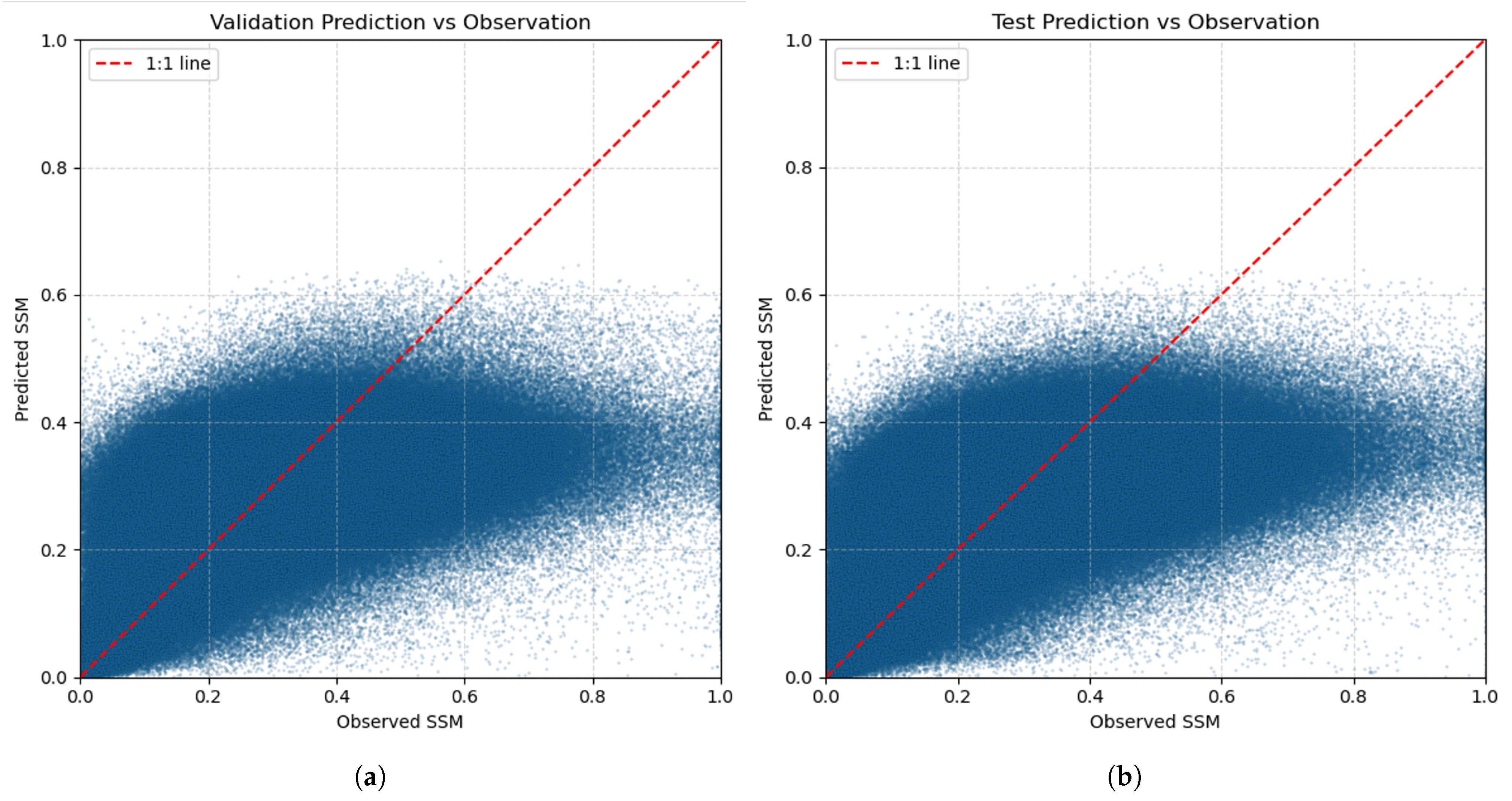
In this study, various model configurations were tested to determine the optimal architecture for accurate SSM prediction. Initially, a 2-layer ConvLSTM model was implemented, but due to its limited performance, the model was increased to five layers as shown in Figure 6. Figure 7 shows the best model performance achieved so far using 2-day weather data (cumulative rainfall and ET and average for other variables).
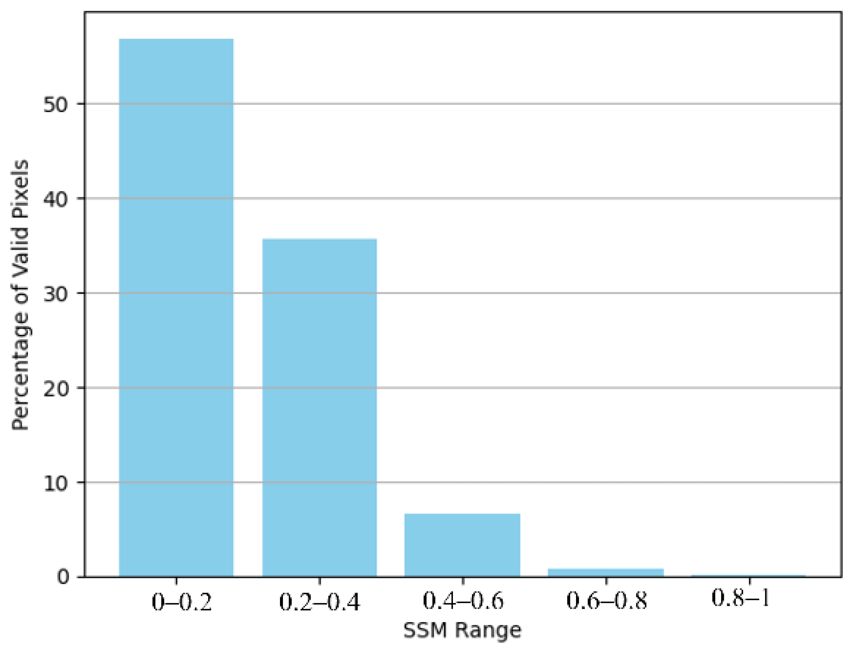
As shown in Figure 7 the model consistently underestimates SSM values above 0.6. To understand the cause of this, a histogram analysis of the training data was conducted (Figure 8). The results show that more than 97% of the SSM values are below 0.6, indicating a strong class imbalance. As a result, the model learns primarily from the majority of data in the lower SSM range, but fails to accurately predict higher values.
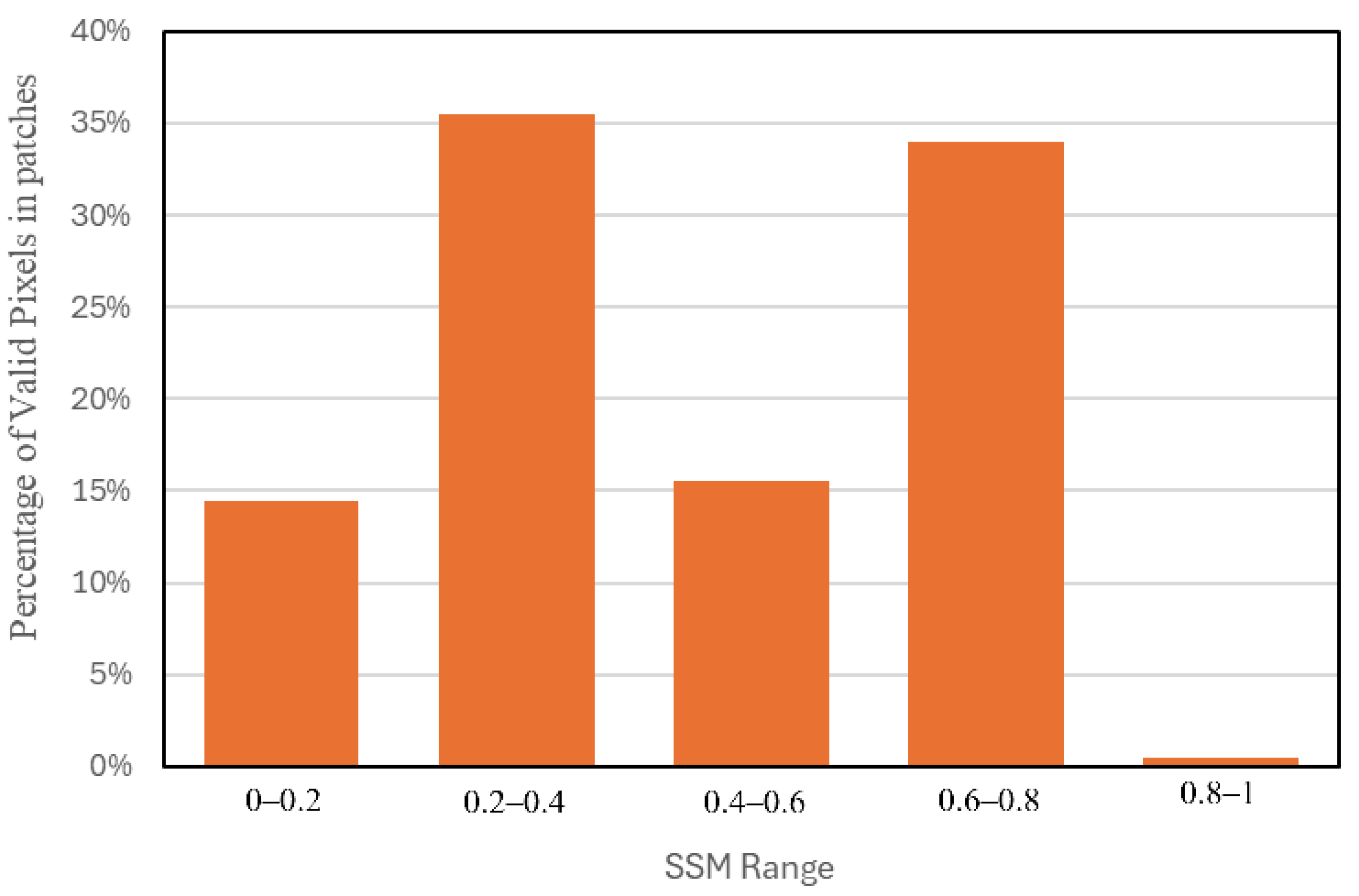
To address the natural imbalance in SSM distributions, a two-pass patch extraction strategy was implemented. By ensuring that more samples with higher SSM values are included in the training data, the model is expected to better learn the full distribution and improve prediction accuracy for underrepresented high SSM values. In the first pass of patch extraction, stratified sampling across the study domain was performed with a coarse stride (i.e., the step size of the pixel used to slide the sampling window), applying class-dependent probabilities to limit oversampling of abundant low-moisture conditions. In the second pass, the high-SSM areas (SSM > 0.6) were explicitly targeted with a dense stride, ensuring a sufficient representation of saturated soils. This approach produced a more balanced and representative training dataset, enhancing the model’s ability to generalize between common and rare hydrological states. Figure 9 shows the distribution of extracted SSM patches after rebalancing.
Table 1 summarizes the evaluation metrics of the models before and after implementing the patch rebalancing strategy. Among the models, the one trained with 2-day weather data demonstrated the highest performance, as indicated by R 2 and correlation values.
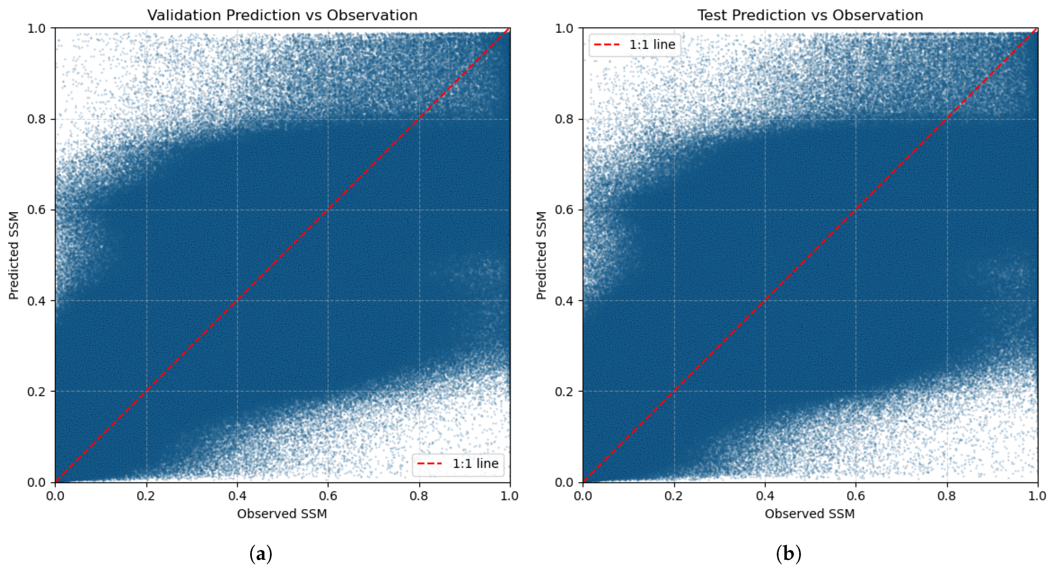
Figure 10 illustrates the predicted SSM values generated by the ML-SSM model using 2-day weather data compared to the observed SSM for both validation and test sets, following the application of the rebalancing strategy for patch generation. As shown in the figure and supported by the evaluation metrics reported in Table 1, the model performance improved substantially after implementing the imbalance correction, demonstrating higher agreement between predicted and observed SSM values and confirming the effectiveness of the patch rebalancing strategy.

3.2. Mapping of Predicted SSM Using ML-SSM Model

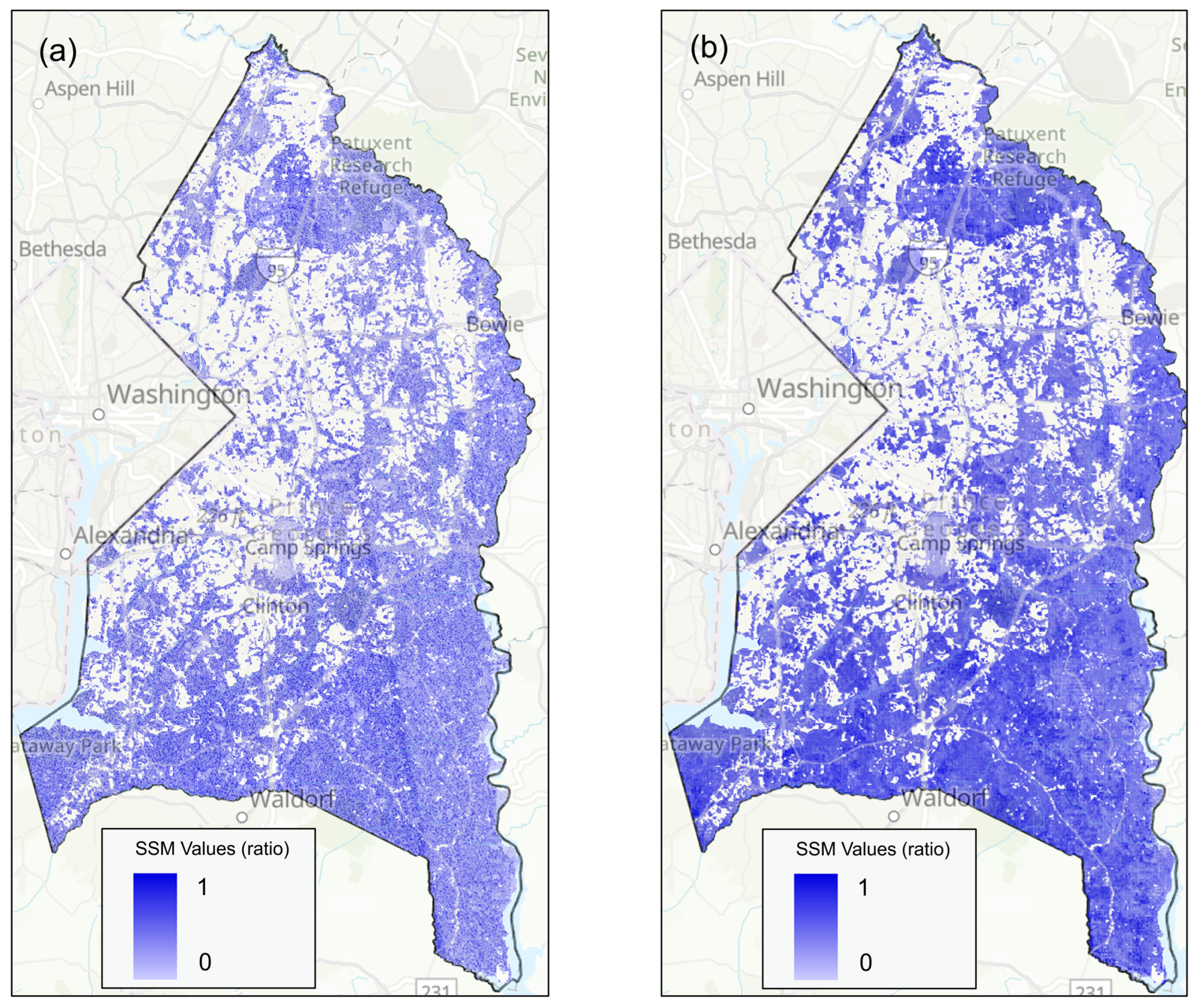
Figure 11 presents the wall-to-wall SSM map predicted by the best-performing ML-SSM model (2-day model) along with the corresponding observed SSM map for a representative date (27 May 2018). A reasonable agreement is observed between the predicted and observation SSM values in different regions of the study area.
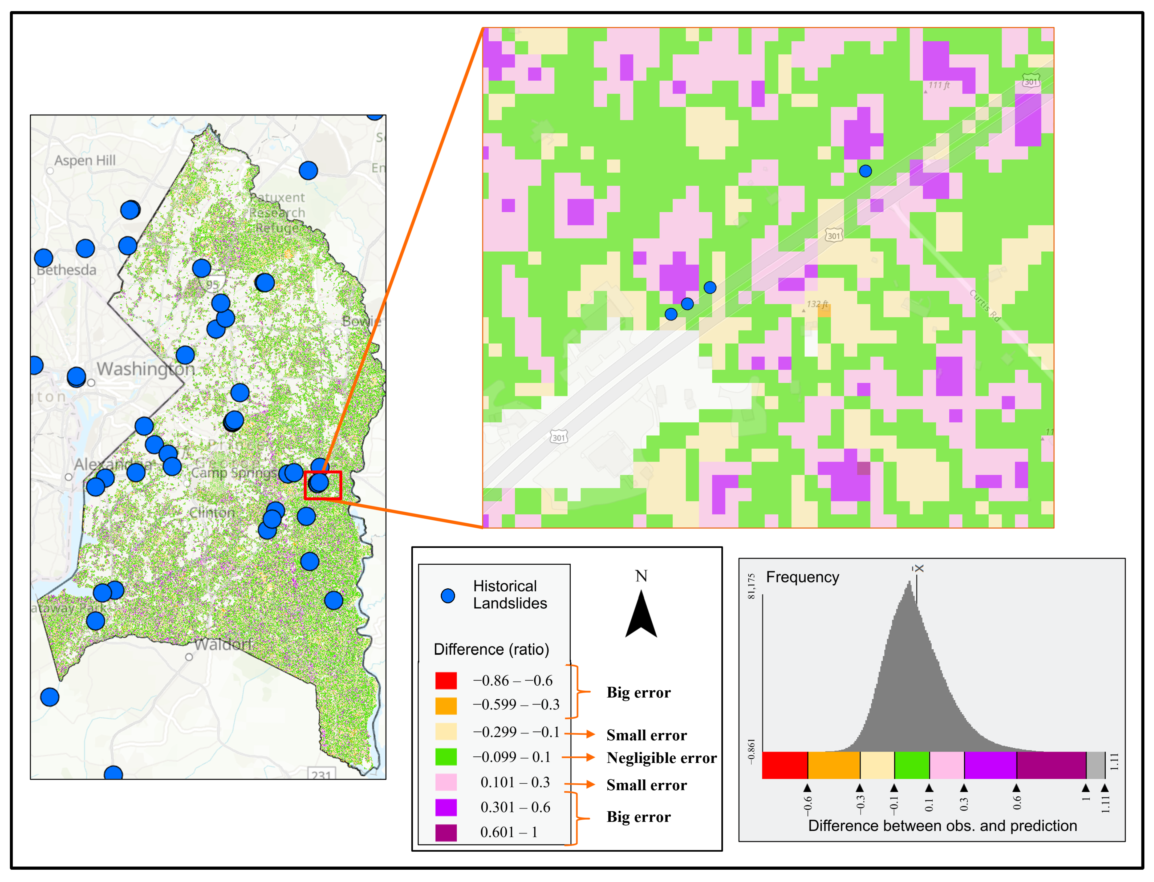
To further evaluate the performance of the ML-SSM model in spatial SSM prediction, a difference map was generated between the observed and predicted SSM values (Figure 12). In this map, negligible differences ( 0.1 to + 0.1 ) are represented in green, and the predominant green areas throughout the case study region indicate strong agreement between observations and predictions. This pattern is quantitatively supported by the histogram of all pixels in the differential map, which shows a distinct peak within the range of 0.1 to + 0.1 . To provide a more detailed view, a zoom-in of a subregion with multiple historical landslide occurrences was analyzed, revealing that all but one of these landslides fall within green areas, corresponding to negligible prediction error. These results demonstrate the reliability of the ML-SSM model in capturing rainfall-induced SSM dynamics and its potential applicability to landslide risk mapping.
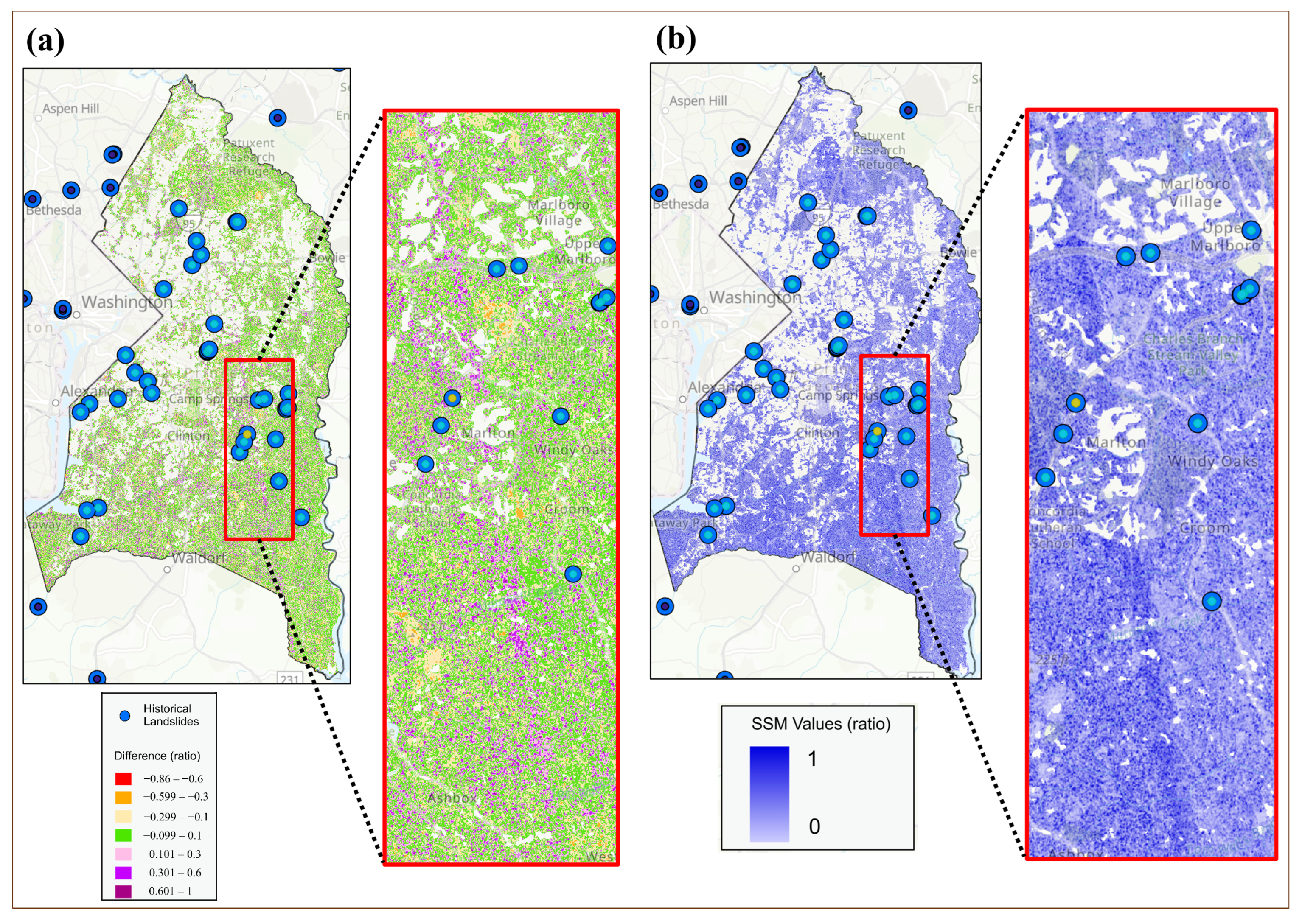
Figure 13 provides a detailed examination of regions with higher prediction error. As shown in part (a), the largest differences between the observed and predicted SSM values, represented in purple, form a distinct linear pattern. A zoom-in of this area confirms the presence of a continuous line of elevated error. To investigate the source of this discrepancy, we included the corresponding observed SSM map in part (b). The same linear feature appears in the observation data, where it consistently shows abnormally high SSM values on multiple dates. Because these SSM maps were derived from Sentinel-1 imagery within the GEE platform, this artifact likely arises from the mosaicking of satellite scenes rather than representing real hydrological conditions. Importantly, the ML-SSM model did not reproduce this linear feature (Figure 11b), as the model was trained on physical input. Therefore the model showed robustness against certain observational artifacts.

4. Conclusions

This study presents a novel deep learning framework for high-resolution spatiotemporal prediction of SSM and demonstrates its potential applicability to rainfall-induced landslide risk assessment in Prince George County, Maryland. Leveraging a ConvLSTM network, the ML-SSM model effectively integrates static terrain and soil properties with multi-temporal meteorological variables and vegetation indices to generate continuous, wall-to-wall SSM maps. The model addresses common limitations of traditional physical and statistical approaches, including sparse in-situ observations, coarse satellite resolution, and oversimplified assumptions regarding infiltration dynamics. The study evaluated three temporal configurations of the input weather data:
  • 1-day model: Uses meteorological variables from the exact observation date of the SSM map.
  • 2-day model: Uses cumulative rainfall and evapotranspiration and averages other variables over the observation date and the preceding day.
  • 3-day model: Extends this to the observation date plus the two preceding days.
Evaluation of the ML-SSM model reveals strong predictive performance, particularly after implementing a two-pass patch extraction strategy to correct class imbalance in high SSM values. Among the configurations tested, the 2-day model achieved the highest performance, with an R 2 of 0.72, a correlation of 0.85, an RMSE of 0.154 and an MAE of 0.103. The model produces SSM maps that closely match the observations derived from Sentinel-1, capturing both spatial and temporal variability in heterogeneous landscapes. Moreover, the ML-SSM framework is robust against artifacts in observational data, such as linear features arising from satellite mosaicking, demonstrating reliable performance across the study area.
These results underscore the significant potential of high-resolution SSM mapping based on ML for hydrological modeling and geohazard mitigation. By providing accurate continuous SSM estimates, the framework can improve landslide early warning systems and inform risk management in regions prone to precipitation-triggered slope failures. The scalable nature of the approach allows a broader application to other geographic areas or environmental contexts, offering a versatile tool for integrating SSM dynamics into environmental modeling and disaster preparedness strategies.
Future work will focus on estimating infiltration based on SSM mapping using the Green–Ampt equation to support physically meaningful hydrological modeling. The timing of the peak SSM will also be determined to identify periods of maximum infiltration, which are critical to assessing the starting time of the landslide. In the final phase of this research, a hybrid physics–machine learning framework will be developed to generate landslide susceptibility maps, bridging the gap between data-driven predictions and physically based slope stability assessments.

Author Contributions

Conceptualization, A.H. and Z.S.; methodology, A.H., Z.S. and Y.L.; software, A.H.; validation, A.H., Z.S. and Y.L.; formal analysis, A.H.; investigation, A.H.; resources, A.H.; data curation, A.H.; writing—original draft preparation, A.H.; writing—review and editing, A.H., Z.S. and Y.L.; visualization, A.H.; supervision, Z.S.; project administration, Z.S.; funding acquisition, Z.S. and Y.L. All authors have read and agreed to the published version of the manuscript.

Funding

This project was sponsored in part by U.S. Department of Transportation National University Transportation Center Safety 21 program (69A3552344811) and Maryland Department of Transportation/State Highway Administration (MDOT/SHA). This project is also supported by the U.S. National Science Foundation (NSF) under Grant No. 2444883 for the project titled CREST-DPSI(S): Expanding a PhD Program in Sustainable and Resilient Infrastructure Engineering.

Data Availability Statement

The datasets presented in this article are not readily available because the data are part of an ongoing study and continue to evolve as the project progresses and mixture of public domain data and generated data and the large size of data sets. Requests to access the datasets should be directed to Zhuping Sheng.

Acknowledgments

ChatGPT (GPT-5.1) is used in this paper for grammatical improvements and proofreading.

Conflicts of Interest

The authors declare no conflicts of interest.

Abbreviations

The following abbreviations are used in this manuscript:
SSMSurface Soil Moisture
MLMachine Learning
ML-SSM     Machine Learning-based Surface Soil Moisture model
MDOTMaryland Department of Transportation
SHAState Highway Administration
USGSUnited States Geological Survey
NASANational Aeronautics and Space Administration
SARSynthetic Aperture Radar
IWInterferometric Wide
VVVertical-Vertical
VHVertical-Horizontal
IDWInverse Distance Weighting method
DEMDigital Elevation Model
SSURGOSoil Survey Geographic Database
GEEGoogle Earth Engine
NDVINormalized Difference Vegetation Index
ESAEuropean Space Agency
ETEvapotranspiration
ConvLSTMConvolutional Long Short-Term Memory
MAEMean Absolute Error
RMSERoot Mean Squared Error

References

  1. Bordoni, M.; Meisina, C.; Valentino, R.; Lu, N.; Bittelli, M.; Chersich, S. Hydrological factors affecting rainfall-induced shallow landslides: From the field monitoring to a simplified slope stability analysis. Eng. Geol. 2015, 193, 19–37. [Google Scholar] [CrossRef]
  2. Galanti, Y.; Barsanti, M.; Cevasco, A.; D’Amato Avanzi, G.; Giannecchini, R. Comparison of statistical methods and multi-time validation for the determination of the shallow landslide rainfall thresholds. Landslides 2018, 15, 937–952. [Google Scholar] [CrossRef]
  3. Zhang, Z.; Zeng, R.; Meng, X.; Zhao, S.; Wang, S.; Ma, J.; Wang, H. Effects of changes in soil properties caused by progressive infiltration of rainwater on rainfall-induced landslides. Catena 2023, 233, 107475. [Google Scholar] [CrossRef]
  4. Zhang, L.; Wu, F.; Zhang, H.; Zhang, L.; Zhang, J. Influences of internal erosion on infiltration and slope stability. Bull. Eng. Geol. Environ. 2019, 78, 1815–1827. [Google Scholar] [CrossRef]
  5. Liu, Q.; Su, L.; Zhang, C.; Hu, B.; Xiao, S. Dynamic variations of interception loss-infiltration-runoff in three land-use types and their influence on slope stability: An example from the eastern margin of the Tibetan Plateau. J. Hydrol. 2022, 612, 128218. [Google Scholar] [CrossRef]
  6. Emberson, R.; Kirschbaum, D.; Stanley, T. New global characterisation of landslide exposure. Nat. Hazards Earth Syst. Sci. 2020, 20, 3413–3424. [Google Scholar] [CrossRef]
  7. Froude, M.J.; Petley, D.N. Global fatal landslide occurrence from 2004 to 2016. Nat. Hazards Earth Syst. Sci. 2018, 18, 2161–2181. [Google Scholar] [CrossRef]
  8. Nelson, S. Slope stability, triggering events, mass movement hazards. Nat. Disasters 2013. Available online: https://amser.org/r7499/slope_stability_triggering_events_mass_wasting_events (accessed on 11 November 2025).
  9. Kirschbaum, D.B.; Stanley, T.; Simmons, J. A dynamic landslide hazard assessment system for Central America and Hispaniola. Nat. Hazards Earth Syst. Sci. 2015, 15, 2257–2272. [Google Scholar] [CrossRef]
  10. Rahardjo, H.; Nistor, M.M.; Gofar, N.; Satyanaga, A.; Xiaosheng, Q.; Chui Yee, S.I. Spatial distribution, variation and trend of five-day antecedent rainfall in Singapore. Georisk Assess. Manag. Risk Eng. Syst. Geohazards 2020, 14, 177–191. [Google Scholar] [CrossRef]
  11. Cevasco, A.; Pepe, G.; Brandolini, P. The influences of geological and land use settings on shallow landslides triggered by an intense rainfall event in a coastal terraced environment. Bull. Eng. Geol. Environ. 2014, 73, 859–875. [Google Scholar] [CrossRef]
  12. Glade, T.; Anderson, M.G.; Crozier, M.J. Landslide Hazard and Risk; Wiley Online Library: Hoboken, NJ, USA, 2005; Volume 807. [Google Scholar]
  13. Zêzere, J.L.; Trigo, R.M.; Trigo, I.F. Shallow and deep landslides induced by rainfall in the Lisbon region (Portugal): Assessment of relationships with the North Atlantic Oscillation. Nat. Hazards Earth Syst. Sci. 2005, 5, 331–344. [Google Scholar] [CrossRef]
  14. Bogaard, T.; Greco, R. Invited perspectives: Hydrological perspectives on precipitation intensity-duration thresholds for landslide initiation: Proposing hydro-meteorological thresholds. Nat. Hazards Earth Syst. Sci. 2018, 18, 31–39. [Google Scholar] [CrossRef]
  15. Kim, J.H.; Fourcaud, T.; Jourdan, C.; Maeght, J.L.; Mao, Z.; Metayer, J.; Meylan, L.; Pierret, A.; Rapidel, B.; Roupsard, O.; et al. Vegetation as a driver of temporal variations in slope stability: The impact of hydrological processes. Geophys. Res. Lett. 2017, 44, 4897–4907. [Google Scholar] [CrossRef]
  16. Özçelik, F.V.; Selçuk, M.E. Parametric Analysis of Factors that Affects the Rainfall Induced Slope Stability. Turk. J. Geosci. 2022, 3, 49–57. [Google Scholar] [CrossRef]
  17. Wu, L.; Zhou, J. Rainfall Infiltration in Unsaturated Soil Slope Failure; Springer Nature: Berlin/Heidelberg, Germany, 2023. [Google Scholar] [CrossRef]
  18. Chen, R.; Chen, H.; Chen, K.; Zhung, H. Simulation of a slope failure induced by rainfall infiltration. Environ. Geol. 2009, 58, 943–952. [Google Scholar] [CrossRef]
  19. Mukhlisin, M.; Taha, M.R. Numerical model of antecedent rainfall effect on slope stability at a hillslope of weathered granitic soil formation. J. Geol. Soc. India 2012, 79, 525–531. [Google Scholar] [CrossRef]
  20. Zhang, J.; Huang, H.W.; Zhang, L.M.; Zhu, H.H.; Shi, B. Probabilistic prediction of rainfall-induced slope failure using a mechanics-based model. Eng. Geol. 2014, 168, 129–140. [Google Scholar] [CrossRef]
  21. Guzzetti, F.; Reichenbach, P.; Ardizzone, F.; Cardinali, M.; Galli, M. Estimating the quality of landslide susceptibility models. Geomorphology 2006, 81, 166–184. [Google Scholar] [CrossRef]
  22. Tung, Y.K.; Zhang, H.; Ng, C.W.W.; Kwok, Y. Transient seepage analysis of rainfall infiltration using a new conjunctive surface-subsurface flow model. In Proceedings of the 57th Canadian Geotechnical Conference and the 5th Joint CGS-IAH Conference, Quebec, QC, Canada, 24–27 October 2004; Volume 7, pp. 17–22. [Google Scholar]
  23. He, W.; Ishikawa, T.; Zhu, Y. Wide/narrow-area slope stability analysis considering infiltration and runoff during heavy precipitation. Soils Found. 2023, 63, 101248. [Google Scholar] [CrossRef]
  24. Chiu, Y.Y.; Chen, H.E.; Yeh, K.C. Investigation of the influence of rainfall runoff on shallow landslides in unsaturated soil using a mathematical model. Water 2019, 11, 1178. [Google Scholar] [CrossRef]
  25. Dolojan, N.L.J.; Moriguchi, S.; Hashimoto, M.; Terada, K. Mapping method of rainfall-induced landslide hazards by infiltration and slope stability analysis: A case study in Marumori, Miyagi, Japan, during the October 2019 Typhoon Hagibis. Landslides 2021, 18, 2039–2057. [Google Scholar] [CrossRef]
  26. Cui, H.; Ji, J.; Hürlimann, M.; Medina, V. Probabilistic and physically-based modelling of rainfall-induced landslide susceptibility using integrated GIS-FORM algorithm. Landslides 2024, 21, 1461–1481. [Google Scholar] [CrossRef]
  27. Chansorn, R.; Chotpantarat, S.; Klongvessa, P. Hydrological model of landslide risk in Huai Nam Phung subbasin, Thailand. Bull. Eng. Geol. Environ. 2023, 82, 140. [Google Scholar] [CrossRef]
  28. Hosseinizadeh, A.; Sheng, Z.; Qian, S.; Liu, Y. Separating Infiltration and Runoff from Precipitation over the Anacostia River Watershed, Maryland. In Proceedings of the World Environmental and Water Resources Congress 2024, Milwaukee, WI, USA, 19–22 May 2024; pp. 1595–1607. [Google Scholar] [CrossRef]
  29. Chaudhary, S.K.; Srivastava, P.K.; Gupta, D.K.; Kumar, P.; Prasad, R.; Pandey, D.K.; Das, A.K.; Gupta, M. Machine learning algorithms for soil moisture estimation using Sentinel-1: Model development and implementation. Adv. Space Res. 2022, 69, 1799–1812. [Google Scholar] [CrossRef]
  30. Chrysanthopoulos, E.; Kallioras, A. Temporal and geographic extrapolation of soil moisture using machine learning algorithms. Catena 2025, 257, 109156. [Google Scholar] [CrossRef]
  31. Acharya, U.; Daigh, A.L.; Oduor, P.G. Machine learning for predicting field soil moisture using soil, crop, and nearby weather station data in the Red River Valley of the North. Soil Syst. 2021, 5, 57. [Google Scholar] [CrossRef]
  32. Gill, M.K.; Asefa, T.; Kemblowski, M.W.; McKee, M. Soil moisture prediction using support vector machines 1. JAWRA J. Am. Water Resour. Assoc. 2006, 42, 1033–1046. [Google Scholar] [CrossRef]
  33. Mittelbach, H.; Seneviratne, S.I. A new perspective on the spatio-temporal variability of soil moisture: Temporal dynamics versus time-invariant contributions. Hydrol. Earth Syst. Sci. 2012, 16, 2169–2179. [Google Scholar] [CrossRef]
  34. Brocca, L.; Melone, F.; Moramarco, T.; Morbidelli, R. Spatial-temporal variability of soil moisture and its estimation across scales. Water Resour. Res. 2010, 46, W02516. [Google Scholar] [CrossRef]
  35. Houben, T.; Ebeling, P.; Khurana, S.; Schmid, J.S.; Boog, J. Machine-learning based spatiotemporal prediction of soil moisture in a grassland hillslope. Vadose Zone J. 2025, 24, e70011. [Google Scholar] [CrossRef]
  36. Jiang, P.; Niu, G.; Li, G. Soil Moisture Prediction Based on Long Short-Term Memory Networks and Meteorological Data. Res. Sq. 2024. [Google Scholar] [CrossRef]
  37. Wang, Y.; Shi, L.; Hu, Y.; Hu, X.; Song, W.; Wang, L. A comprehensive study of deep learning for soil moisture prediction. Hydrol. Earth Syst. Sci. Discuss. 2023, 28, 917–943. [Google Scholar] [CrossRef]
  38. Ahmad, S.; Kalra, A.; Stephen, H. Estimating soil moisture using remote sensing data: A machine learning approach. Adv. Water Resour. 2010, 33, 69–80. [Google Scholar] [CrossRef]
  39. Senyurek, V.; Lei, F.; Boyd, D.; Kurum, M.; Gurbuz, A.C.; Moorhead, R. Machine learning-based CYGNSS soil moisture estimates over ISMN sites in CONUS. Remote Sens. 2020, 12, 1168. [Google Scholar] [CrossRef]
  40. Vereecken, H.; Huisman, J.; Pachepsky, Y.; Montzka, C.; Van Der Kruk, J.; Bogena, H.; Weihermüller, L.; Herbst, M.; Martinez, G.; Vanderborght, J. On the spatio-temporal dynamics of soil moisture at the field scale. J. Hydrol. 2014, 516, 76–96. [Google Scholar] [CrossRef]
  41. Entekhabi, D.; Njoku, E.G.; O’Neill, P.E.; Kellogg, K.H.; Crow, W.T.; Edelstein, W.N.; Entin, J.K.; Goodman, S.D.; Jackson, T.J.; Johnson, J.; et al. The Soil Moisture Active Passive (SMAP) mission. Proc. IEEE 2010, 98, 704–716. [Google Scholar] [CrossRef]
  42. Batchu, V.; Nearing, G.; Gulshan, V. A machine learning data fusion model for soil moisture retrieval. arXiv 2022, arXiv:2206.09649. [Google Scholar] [CrossRef]
  43. Liu, Y.; Jing, W.; Wang, Q.; Xia, X. Generating high-resolution daily soil moisture by using spatial downscaling techniques: A comparison of six machine learning algorithms. Adv. Water Resour. 2020, 141, 103601. [Google Scholar] [CrossRef]
  44. Torres, R.; Snoeij, P.; Geudtner, D.; Bibby, D.; Davidson, M.; Attema, E.; Potin, P.; Rommen, B.; Floury, N.; Brown, M.; et al. GMES Sentinel-1 mission. Remote Sens. Environ. 2012, 120, 9–24. [Google Scholar] [CrossRef]
  45. Miranda, N.; Torres, R.; Geudtner, D.; Pinheiro, M.; Potin, P.; Gratadour, J.B.; O’Connell, A.; Bibby, D.; Navas-Traver, I.; Cossu, M. Sentinel-1 First Generation Status, Past and Future. In Proceedings of the IGARSS 2023—2023 IEEE International Geoscience and Remote Sensing Symposium, Pasadena, CA, USA, 16–21 July 2023; IEEE: New York, NY, USA, 2023; pp. 4560–4563. [Google Scholar] [CrossRef]
  46. Massart, S.; Vreugdenhil, M.; Bauer-Marschallinger, B.; Navacchi, C.; Raml, B.; Wagner, W. Mitigating the impact of dense vegetation on the Sentinel-1 surface soil moisture retrievals over Europe. Eur. J. Remote Sens. 2024, 57, 2300985. [Google Scholar] [CrossRef]
  47. Li, J.; Heap, A.D. A Review of Spatial Interpolation Methods for Environmental Scientists; Geoscience Australia: Canberra, Australia, 2008. [Google Scholar]
  48. Drusch, M.; Del Bello, U.; Carlier, S.; Colin, O.; Fernandez, V.; Gascon, F.; Hoersch, B.; Isola, C.; Laberinti, P.; Martimort, P.; et al. Sentinel-2: ESA’s optical high-resolution mission for GMES operational services. Remote Sens. Environ. 2012, 120, 25–36. [Google Scholar] [CrossRef]
  49. Pettorelli, N.; Vik, J.O.; Mysterud, A.; Gaillard, J.M.; Tucker, C.J.; Stenseth, N.C. Using the satellite-derived NDVI to assess ecological responses to environmental change. Trends Ecol. Evol. 2005, 20, 503–510. [Google Scholar] [CrossRef]
  50. Wagner, W.; Lemoine, G.; Rott, H. A method for estimating soil moisture from ERS scatterometer and soil data. Remote Sens. Environ. 1999, 70, 191–207. [Google Scholar] [CrossRef]
  51. Bauer-Marschallinger, B.; Freeman, V.; Cao, S.; Paulik, C.; Schaufler, S.; Stachl, T.; Modanesi, S.; Massari, C.; Ciabatta, L.; Brocca, L.; et al. Toward global soil moisture monitoring with Sentinel-1: Harnessing assets and overcoming obstacles. IEEE Trans. Geosci. Remote Sens. 2018, 57, 520–539. [Google Scholar] [CrossRef]
  52. van Hateren, T.C.; Chini, M.; Matgen, P.; Pulvirenti, L.; Pierdicca, N.; Teuling, A.J. On the potential of Sentinel-1 for sub-field scale soil moisture monitoring. Int. J. Appl. Earth Obs. Geoinf. 2023, 120, 103342. [Google Scholar] [CrossRef]
  53. Shi, X.; Chen, Z.; Wang, H.; Yeung, D.Y.; Wong, W.k.; Woo, W.c. Convolutional LSTM network: A machine learning approach for precipitation nowcasting. In Proceedings of the Advances in Neural Information Processing Systems, Montreal, QC, Canada, 7–12 December 2015; Curran Associates, Inc.: Vancouver, BC, Canada, 2015; Volume 28, pp. 802–810. [Google Scholar]
  54. Ulloa, N.I.; Yun, S.H.; Chiang, S.H.; Furuta, R. Sentinel-1 spatiotemporal simulation using convolutional LSTM for flood mapping. Remote Sens. 2022, 14, 246. [Google Scholar] [CrossRef]
  55. ElSaadani, M.; Habib, E.; Abdelhameed, A.; Bayoumi, M. Assessment of a Spatiotemporal Deep Learning Approach for Soil Moisture Prediction. Front. Artif. Intell. 2021, 4, 636234. [Google Scholar] [CrossRef] [PubMed]
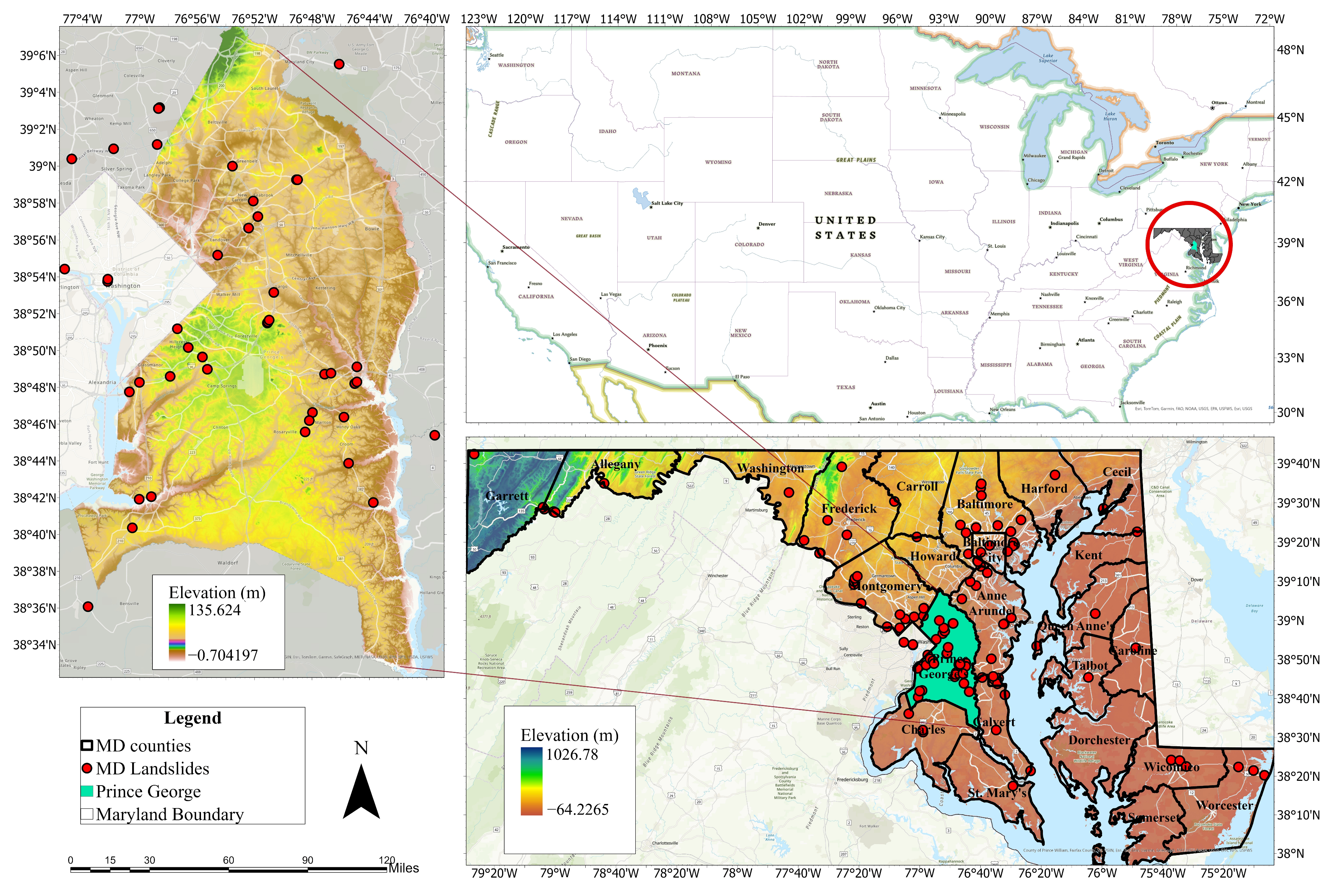
Figure 1. Historical landslide location in Maryland and the selected case study area, Prince George County.
Water 17 03300 g001
Figure 2. Landslide analysis in Maryland: (a) Number of landslides by county; (b) Annual precipitation vs. number of landslides; (c) Three-day cumulative rainfall vs. number of landslides; (d) Surface soil moisture (from Open-Meteo) vs. number of landslides.
Water 17 03300 g002
Figure 3. Workflow chart of the research.
Water 17 03300 g003
Figure 4. Spatial distribution of weather observation points from the Open-Meteo database used for interpolation.
Water 17 03300 g004
Figure 5. Input data to ML-SSM model: (a) Rainfall; (b) Maximum temperature; (c) Minimum temperature; (d) Relative humidity; (e) Wind speed; (f) Evapotranspiration; (g) NDVI; (h) Elevation; (i) Slope angle; (j) Silt content; (k) Clay content; (l) Sand content.
Water 17 03300 g005
Figure 6. ConvLSTM model architecture used in the ML-SSM framework.
Water 17 03300 g006
Figure 7. Predicted SSM values by ML-SSM model using the 2-day weather data versus observed SSM for (a) Validation set and (b) Test set.
Water 17 03300 g007
Figure 8. Original SSM data histogram and distribution.
Water 17 03300 g008
Figure 9. SSM data histogram and distribution using two-pass patch extraction strategy.
Water 17 03300 g009
Figure 10. Predicted SSM values by ML-SSM model using the 2-day weather data versus observed SSM for (a) Validation set and (b) Test set after applying the rebalancing strategy for patch generation.
Water 17 03300 g010
Figure 11. Wall to wall SSM maps for (a) observation data and (b) predicted values using 2-day ML-SSM model in 27 May 2018.
Water 17 03300 g011
Figure 12. Difference between prediction and observation SSM maps in 27 May 2018.
Water 17 03300 g012
Figure 13. Zoom-in view of (a) the difference between prediction and observation SSM maps and (b) observation SSM map in 27 May 2018.
Water 17 03300 g013
Table 1. Model performance metrics before and after rebalancing.
MetricRebalance1-Day Model2-Day Model3-Day Model
Training Validation Test Training Validation Test Training Validation Test
R2Before0.21350.20350.20760.19360.18340.19170.19920.18960.1970
After0.71700.71370.71660.72240.71730.71710.72040.71220.7151
RMSEBefore0.14920.15040.14980.15110.15230.15130.15060.15180.1508
After0.15200.15300.15190.15230.15370.15410.15280.15500.1547
MAEBefore0.11390.11480.11460.11480.11570.11510.11480.11560.1152
After0.10160.10210.10140.10210.10290.10330.10290.10450.1040
CorrelationBefore0.46640.45720.45960.45100.44150.44850.45220.44330.4492
After0.84710.84520.84690.85080.84770.84890.84890.84420.8459
Note: The bold values are for better models (higher R 2 and Correlation and lower error RMSE and MAE).
Disclaimer/Publisher’s Note: The statements, opinions and data contained in all publications are solely those of the individual author(s) and contributor(s) and not of MDPI and/or the editor(s). MDPI and/or the editor(s) disclaim responsibility for any injury to people or property resulting from any ideas, methods, instructions or products referred to in the content.