Abstract
This article presents an analysis of the changes in hydrogeological parameters considering borehole efficiency. The first part presents the initial assumptions and methodology for determining hydraulic and hydrogeological parameters. Then, the results of parameter changes analysis are presented for 40 cases of water wells which have been occurring over several decades of their operation. The tested wells were drilled in porous aquifers—Quaternary and Neogene sands—as well as fissured aquifers—Cretaceous marls, Jurassic limestones and marls, and Triassic limestones and dolomites. They were divided into groups depending on the type of aquifer medium and the nature of the damage. Group 1 includes wells where water contamination occurred and where changes in hydraulic parameters suggested damage of a critical nature. Group 2 includes wells with a marked increase inflow resistance where advanced clogging was proposed. In Group 3, the changes were similar, but the extent was not as advanced. The efficiency curves analysis and step-drawdown test results made it possible to determine parameters such as hydraulic conductivity, penetration ratio, well-screen transmissivity and current critical well-yield. The calculation methodology used indicates the types and causes of damage and allows a preliminary assessment of the chance of rehabilitating the object in accordance with the principle of sustainable management of environmental resources and technical assets. Alternatively, it allows for the selection of more detailed or invasive diagnostic tests.
1. Introduction
Water wells play a crucial role in hydrogeological studies, providing essential data for evaluating groundwater resources and system dynamics. The efficiency of a well directly influences the accuracy of hydrogeological parameter assessments, including hydraulic conductivity, transmissivity and penetration ratio. Poorly performing wells can cause significant errors in data interpretation, leading to incorrect conclusions regarding aquifer properties and water availability. Additionally, efficiency-related issues can help identify structural defects such as clogging, casing corrosion or improper well development. This article explores the relationship between well efficiency, the reliability of hydrogeological assessments and defect detection, highlighting the need for proper well construction, maintenance and performance monitoring.
Efficiency is a technical term describing the effect achieved in relation to the effort expended. In the case of a hydrogeological borehole, the efficiency factor can be expressed as the ratio between the water table depression in the aquifer and the depression measured inside the borehole. The difference in position of the water table is known as the well-loss, which is a measure of hydraulic losses. Furthermore, it explains the difference between the theoretical water table and the actual state.
The condition of the borehole can be assessed in various ways. The most common methods are visual inspections using a TV camera, geophysical measurements and tests, pumping tests, etc.
The assessment of the effectiveness of well development was proposed by Walton [1]. The author has suggested a classification of wells based on the non-laminar loss coefficient. The well efficiency curves were proposed by Bierschenk [2] based on 46 wells drilled in Iran and the State of Washington, USA. This study notes that technical efficiency is influenced by the natural transmissivity of the aquifer. Kurtulus et al. [3]. proposed a tabular classification based on the non-laminar well-loss coefficient and the P power exponent.
There are many publications which have focused on the non-laminar well-loss coefficient as the value of this component that is influenced only by technical factors. These include the drilling method, borehole diameter, penetration ratio, well-screen type and clogging progression [4,5,6,7].
Houben noticed that “the single most important contributor to drawdown is commonly the aquifer. Its hydraulic conductivity can only be improved slightly through development” [8]. Since laminar aquifer loss is a factor dependent on hydrogeological conditions, this component was omitted from the assessment of borehole efficiency. Many methods for processing measurement data can be found in the literature, e.g., [1,9,10,11,12,13,14,15], as well as methods for determining aquifer drawdown and well-loss, e.g., [16,17,18,19].
An important groundwater abstraction assessment technique is the step-drawdown test (SDT). An SDT typically involves pumping at a constant rate Q, while continuously monitoring water level drawdown S within the abstraction well. Eventually, the water level is expected to reach a quasi-steady state. Once this occurs, the abstraction rate is increased and held constant until a new quasi-steady state is achieved [20].
An SDT is a single-well test in which the well is pumped at a low constant discharge rate until the drawdown within the well-tube stabilizes. Then, the procedure is repeated at a higher constant discharge rate for at least three steps. The duration of each step should be equal for 30 to 120 min. The details for data collection and solving the equations are presented in [21].
Polak et al. [22] noticed that maintaining a constant flow rate is not necessary. The water table decrease inside the well-tube interacts with a pump head increase, in accordance with the slope of the pump curve. This causes a decrease in a flow rate. The drawdown interacts with flow velocity v in any circular cross-section L with a diameter 2r, where the well is the central point of the system. The flow rate increase limits further increase in drawdown. The time required to stabilize the conditions therefore depends on the rate of propagation of the cone of depression, i.e., on the permeability of both the well-filter and the aquifer. An SDT duration is dependent on both hydrogeological and hydraulic conditions, including the slope of the pump curve. It can take from 12 min to a few hours.
Paper [23] presents a method for conducting an SDT for a partially penetrating well with irregular (non-linearly increasing) pumping rates. The new coefficient, the pumping rate varying index α, was introduced to indicate the pumping rate difference (ΔQ) between the two steps.
The method and the research presented in the next sections of this paper have certain limitations. They can be applied to wells that capture one aquifer. Otherwise, multilevel pumping test is required. The basis for further research is that the reference SDT is usually conducted during the acceptance of the borehole from the contractor.
2. Methods
A calculation scheme for quasi-steady-state conditions, simplified from the actual groundwater flow conditions, describes the movement of groundwater into a well. It assumes that the well is fully penetrated and that the borehole diameter is relatively small. The borehole operates at a constant pumping rate in a homogeneous aquifer with infinite extent. The aquifer, in this case, has a constant thickness. Water flow is laminar and radial. The water inflow into a well for a confined aquifer is described by the Dupuit [24] equation as follows:
For an unconfined aquifer, the equation takes the following form:
where
- K—hydraulic conductivity, [LT−1]
- m—thickness of confined aquifer, [L]
- R—radius of influence zone, [L]
- r—borehole diameter, [L]
- H—hydraulic head of unconfined aquifer, [L]
- S—water table depression, [L].
The observed drawdown indicates a lowering of the water table in the well, not in the aquifer. The relationship between well drawdown and flow rate is described by the Rorabaugh [25] equation:
where
- B—linear well-loss coefficient, [TL−2]
- C—non-linear well-loss coefficient, [T2L−5]
- SL—linear drawdown, [L]
- P—exponent can assume values of 1.5 to 3.5, depending on Q, [-].
These types of conditions are usually observed in wells capturing water from a fractured aquifer and at relatively high flow rates. The efficiency η of a well can then be described by the equation:
The form of a marked function can be described in the following way [26]:
where
A special case is the state in which the exponent of the power P is 2. The equation follows a form that is consistent with the notation previously proposed by Jacob [27]. Methods for determining the parameters of the equation are described in numerous publications [17,28,29,30,31].
The efficiency curve of the opening reaches its maximum, equal to 100%, at a flow rate of 0. As the well-yield increases, the efficiency decreases. The deflection of the curve depends on the ratio of the turbulent flow coefficient to the laminar flow coefficient α. This means that the efficiency of the borehole is determined by factors depending on the construction of the borehole and the degree of filter clogging, as well as the natural permeability of the aquifer. However, the permeability is a constant or slowly changing value over time.
Establishing the efficiency curve allows us to assess hydraulic and hydrogeological parameters for any period of the well’s life. It is possible to evaluate the degree of degradation of the borehole as well as the changes in the aquifer over any given period by comparing the results. Considering the following:
it is possible to determine the hydraulic conductivity of the aquifer. In particular, corrections for the well penetration ratio b and the efficiency corresponding to the well-yield must also be considered.
where
- b—penetration ratio of the aquifer, [-]
- η—well efficiency corresponding to pumping rate in steady-state flow, [-].
According to Forchheimer [32], the aquifer penetration ratio for a confined aquifer can be expressed as follows:
where
- l—length of well screen, [L].
In an unconfined aquifer, the value of the penetration ratio can be calculated by the formula:
Formulas (8) and (9) contain values that are significantly dependent on pumping rate. In addition to water table depression, which can be measured directly, there is also the radius of influence zone R. It is defined as the boundary of the cone of depression and means the distance from the centre of a well to the point where there is no lowering of the water table or potentiometric surface [33] or beyond which drawdown is negligible or unobservable [34]. The radius of influence is determined by indirect measurement in an observation well or approximated arithmetically.
The Sichardt formula for the radius of influence for confined aquifers [35], when well efficiency is taken into account, has the following form:
The Kusakin formula for unconfined aquifers [33], when well efficiency is taken into account, has the following form:
where
- B, Q—in consistent units of measurement,
- K—the hydraulic conductivity in m/s.
The calculation of parameters K and R can be performed using the successive approximation method. According to Louwyck et al. [36], the original Sichardt formula estimates the radius of influence by simply considering the aquifer hydraulic conductivity and drawdown in the pumping well. It tends to underestimate the extent of the cone of depression. However, the results of model research carried out by El-Hames [37] indicate that the results produced by the Sichardt and Kusakin methods are not accurate and are greatly overexaggerated, leading to much bigger values of the radius of influence.
It should be noted here that the authors mentioned above omit the well efficiency ratio in their considerations due to their neglecting hydraulic losses. This leads to different and inappropriate conclusions. It should be emphasized that the results of calculations performed using the original Sichadt and Kusakin formulas are correct only for wells with a high hydraulic efficiency ratio.
Taking into account the previous considerations, the final Dupuit–Forchheimer formula for both types of aquifers can be written as:
for a confined aquifer, and:
for an unconfined aquifer.
The extent of the cone of depression, in both cases, is slightly underestimated, as it does not take into account the extent of the non-linear flow zone. Motyka and Wilk [38] showed that the radius of a non-linear zone usually develops directly around the well, especially for fractured karstic rocks. Since its extent is small when compared to the extent of the linear flow zone, this value can be disregarded.
2.1. Specific Drawdown of the Well
The specific drawdown of the well is the ratio of the observed depression to the flow rate. It can be expressed by the formula:
For correctly constructed and equipped wells, the function S/Q = f(Q) can take one of three shapes. Their types are illustrated in Figure 1. If the exponent P in Equation (3) takes a value equal to 1, then the flow follows the Dupuit assumption (Curve 1). When the exponent of power is equal to 2, the flow is linear in the aquifer and mixed in the gravel-pack zone (Curve 2). The final case is the most common, which involves the development of turbulence into an aquifer near-borehole zone (Curve 3).
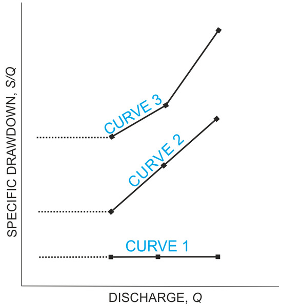
Figure 1.
Typical drawdown curve types, based on those recommended by Atkinson et al. [39]; solid line—misured, dash line—suspected.
When considering the efficiency of the well η, it is worth noting that the specific drawdown is representing the aquifer laminar flow coefficient B, as follows.
2.2. Specific Well-Yield
The specific yield q1 is the opposite of the specific drawdown of the well, also called the productivity of the well. When η = 1, the specific yield expresses both the conductivity of the aquifer T and the well T′. In other words, if a well has 100% efficiency, its well-yield is equal to the aquifer transmissivity. This case is represented by Line (Curve) 1 in Figure 1. It could be expressed as follows:
When the efficiency of the well η < 1, the ratio Q/S expresses the specific well-yield T′ only. Considering well efficiency, the hydraulic properties of the aquifer can be determined as follows:
An example of the results is shown in the figure below (Figure 2).
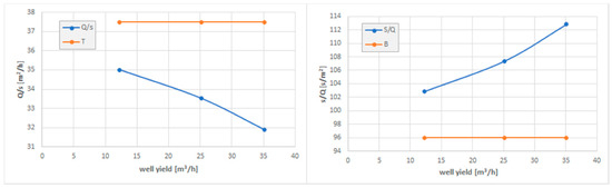
Figure 2.
Transmissivity T and linear well-loss coefficient B for the chosen water well (for better readability, T expressed in m2/h, B expressed in s/m2).
This implies that T and B are constant values regardless of the pumping rate, as well as q(T) ≥ q1(T′). The cases represent Lines (Curves) 2 and 3 in Figure 1.
2.3. Aquifer Penetration Ratio
Once the hydraulic conductivity has been calculated, it is possible to evaluate the aquifer penetration ratio b. For confined aquifers, this is equal to:
Considering Equation (19), it can be written that:
For an unconfined aquifer, it could be described as follows:
It follows that the penetration ratio can be determined by considering the well efficiency at the current pumping rate in relation to steady-state conditions, i.e., when the cone of depression is fully stabilized.
2.3.1. Well Transmissivity
It is worth noting that, when the efficiency of the well is considered, the specific well-yield T′ is related to the aquifer transmissivity T that follows:
2.3.2. Critical Well-Yield
As can be seen above, the well-screen penetration ratio contributes to a reduction in well-screen transmissivity. The critical flow rate is decreased because of this reduction. With this in mind, a correction can be made to the permissible well-yield formula. Therefore, the critical water velocity for wells operating temporarily (with operational interruptions) formula defined by Sichardt [35] requires correction, as follows:
On the other hand, Truelsen’s formula for wells operating continuously (24 h per day) [40] can be written as the following:
Finally, appropriate to the mode of operation, the critical well-yield Qcrit is as follows:
where
- D—borehole diameter, [L]
- L—well-screen length, [L].
3. Materials
The study material contained wells that featured both fissure and porous aquifers. All wells were numbered from 1 to 40. In the following sections of this paper, these symbols are used uniformly on schematic maps, in figures and in tables.
Firstly, the initial parameters were determined in the following sequence: B and C, K and R, Qcrit, T, T′, b. For this purpose, archival material was used, which included the results of step-drawdown tests carried out after the drilling work was completed. In each case, a final step-drawdown test was carried out to identify the cause of the problem.
The Q and S data samples from all 40 boreholes are fitted using Equation (3). The coefficient of determination of the models is R2 > 0.95. The geometry of the boreholes and the lithology of the aquifers are derived from drilling data.
If the SDT data samples contained errors regarding Equation (3), the experiments were repeated. Correctly verified SDT results were not repeated.
The wells in which the tests were carried out were located in various regions of Poland. They belonged to various groundwater reservoirs and differed in depth and construction. During the preliminary analysis, no spatial correlation was found in terms of borehole efficiency. Their locations are shown on a schematic map—Figure 3.
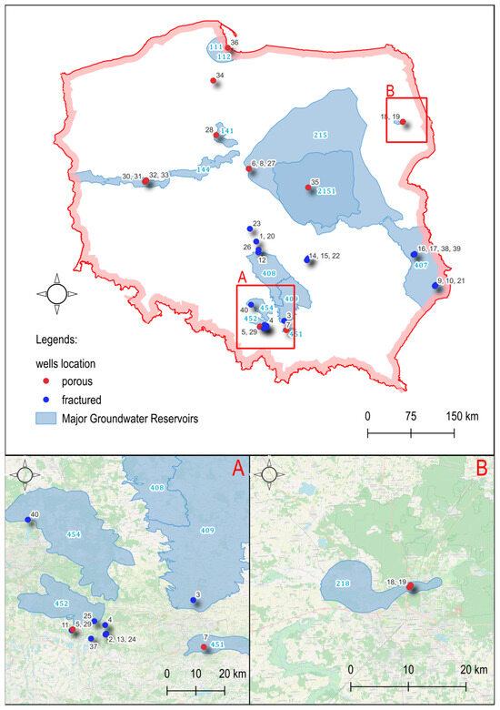
Figure 3.
Location of tested water wells. Explanations: Major Grandwater Reservoirs (MGR): No 111, 112—well 36 (quarternery sands); No. 141—well 28 (quarternery sands); No. 144—wells 30, 31, 32, 33 (quarternery sands); No. 215—wells 6, 8, 27, 35 (quarternery sands); No. 218—wells 18, 19 (quarternery sands); No. 407—wells 9, 10, 16, 17, 21, 38, 39 (cretaceous marls); No. 408—well 12 (jurassic limestones); No. 409—well 3 (cretaceous marls); No. 451—well 7 (neogene sands); No. 452—well 25 (triasic dolomites and limestones); No. 454—well 40 (triasic limestones). The local aqiufer out of MGR: wells 5, 29, 34, 37—quarternery sands; wells 1, 2, 4, 13, 14, 15, 20, 22, 23, 24, 26—jurrasic limestones; well 11—carboniferous sandstones.
3.1. Fractured Aquifers
The study sample consisted of wells supplying water to a public water supply system. Generally, they operate temporarily, supplying the retention reservoirs. The calculations carried out revealed that only 3 out of 25 wells had an initial efficiency equal to 1. All these boreholes (wells no. 1, 14, and 39) encountered rock layers of considerable thickness and secondary porosity by solution opening. Two of them are open-hole wells, and the last one has been equipped with a high perforated well screen. It is possible to conclude that, initially, the water supply followed the Dupuit scheme in these cases. However, in all cases, the efficiency was determined using Equation (5). Figure 4 shows the initial efficiency curves, and then the final curves are shown in Figure 5. Coloured points on this figure are critical well-yields relating to Table 1.
Figure 4.
Initial efficiency curves for water wells in fractured aquifers.
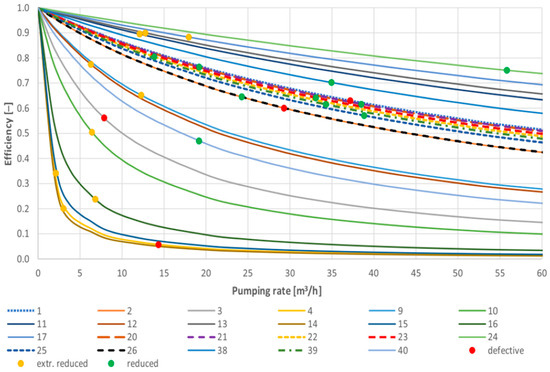
Figure 5.
Final efficiency curves of water wells in fractured aquifers.

Table 1.
Hydraulic parameters for fractured aquifer wells marked in blue in Figure 3.
Repetition of pumping tests indicated that all wells had significant hydraulic resistance coefficients. Therefore, the efficiency curves have been re-determined using Equation (5). Hydrogeological parameters were then calculated and analyzed. Considering the final and initial parameters of each site, the results were compared, and an interpretation was made of the changes that occurred during the period of operation.
3.2. Porous Aquifers
Similarly to above, wells were supplying water for public purposes. The calculations carried out revealed that only 2 of the 15 wells had an initial efficiency equal to 1. In both cases, the seasonal presence of bacteria and microorganisms in the water was observed during the operation time. It can be assumed that the high efficiency was related to the failure of the annular borehole seal between the near-surface aquifers and the production aquifer. Figure 6 shows the initial efficiency curves, and then the final curves are shown in Figure 7. Coloured points on this figure are critical well-yields relating to Table 2.
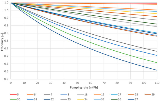
Figure 6.
Initial efficiency curves for water wells in porous aquifers; vertical axis from 0.5 to 1.0.
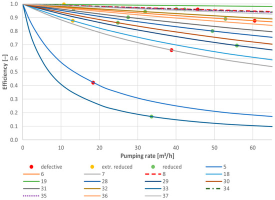
Figure 7.
Final efficiency curves of water wells in porous aquifers.
Table 2.
Hydraulic parameters for porous aquifer wells marked in red in Figure 3.
4. Results
Using initial efficiency curves, the following initial hydrogeological parameters were determined: hydraulic conductivity K, aquifer transmissivity T, and well-screen penetration ratio b (Figure 8 and Figure 9).
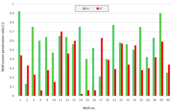
Figure 8.
Initial (bo) and final (bf) fractured aquifers penetration ratio.
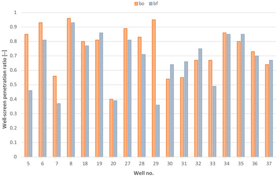
Figure 9.
Initial (bo) and final (bf) porous media penetration ratio.
The repeated pumping test was performed at no less than three step-drawdown steps. The objective was to update efficiency curves and estimates of hydrogeological parameters. By comparing the results obtained, the causes of the failures were determined, and the possibility of renovating or reconstructing the boreholes was assessed.
The study of the wells was conducted in three groups, bearing in mind the causes of inefficiency noticed by the water public supplier during many years of operation. These were primarily the following:
- The appearance of bacteria, microorganisms, and mechanical pollutants in the water (Group 1).
- Significant reduction in operational performance was observed in (Group 2).
- Moderate reduction in operational parameters (Group 3).
The calculation’s results are summarized in Table 1 and Table 2. The data presented include the final parameters characterizing the test facilities after the end of the operating period. The average lifetime, between pumping tests, is more than 38 years.
- Wells in Group 1 are characterized by a reduction in laminar flow resistance coefficient over time.
- Wells in Group 2, except well 15, are characterized by a very high increase in the turbulent flow resistance coefficient. Reduction in the laminar flow resistance coefficient were detected in only three wells (no. 14, 15, and 16). However, this did not result in water contamination.
- In wells in Group 3, changes in coefficients B and C are not as significant as in Groups 1 and 2.
5. Discussion
A decrease in laminar flow resistance may be related to the removal of residual muds at the beginning of the operational stage or to well-seal damage. In this second case, the origin of the pollution in the surface water or shallow unconfined layer seepage is concerning. At the same time, there is usually an increase in the borehole efficiency and the well penetration ratio.
A natural process concerned with well operation is well-screen clogging. It manifests itself in the form of increased hydraulic resistance coefficients, where, unlike coefficient C, coefficient B is slow-loading. So, a stable increase in the B value over time is a natural and expected process. However, the reduction in the turbulent flow resistance C coefficient is also observed, as an effect of well-screen or well-seal disintegration.
The analysis of wells in Group 1 (no. 1 ÷ 8), in which water contamination occurred, shows that some major changes in parameters took place:
- -
- There was a significant decrease in the penetration ratio b in almost all the wells (with the exception of well no. 2).
- -
- In all the wells drilled in porous aquifer, the well-yield increased, while in the fissured aquifer, the well-yield increased only in one well.
- -
- Efficiency increased significantly, with the exception of wells no. 2 and no. 8.
- -
- There was an improvement in laminar flow conditions in all the wells.
The deterioration in the physicochemical and bacteriological quality parameters of the water is caused by well-seal damage. As a result, water from contaminated aquifers has entered the system.
The analysis of wells in Group 2 (no. 9 ÷ 19) shows that some wells have similar parameter changes to those in Group 1. However, there is no water quality deterioration. These are wells 9, 10, 14, 15, 16. The following changes have occurred in these wells:
- -
- a decrease in the penetration ratio;
- -
- there was a moderate increase in laminar flow resistance and an improvement in hydraulic conductivity K, in wells no. 9 and 10;
- -
- there was a decrease in laminar flow resistance in wells 14, 15, and 16.
Wells no. 14, 15, and 16 are very interesting cases. Despite initially positive hydraulic parameters, the hydraulic conductivity of the aquifer was improved and the boreholes became clogged. This is manifested by a very low final penetration ratio. In each case, the direct cause was an overestimation of the well-yield and operation at too high a hydraulic gradient, i.e., low efficiency. These three above-mentioned wells had a critical well-yield of 17% of the primary pumping rate. The other wells in Figure 10, which experienced a reduction in their critical well-yield, have a well-yield of 60% of the initial pumping rate.
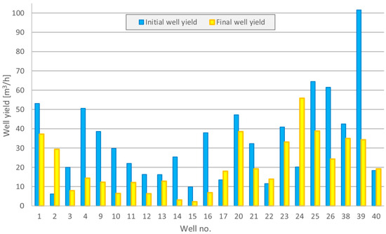
Figure 10.
Initial and final well-yields, fractured aquifers.
In the remaining wells in Group 2, the changes are not so significant. In some wells, for example no. 20 and 22, there was a slight decrease in the penetration ratio at the expense of hydraulic conductivity improvement.
The largest increase in critical well-yield is in wells no. 2 and 24. These wells are located a short distance from each other and water is extracted from the same karstic formations. The removal of backfill from the between-gap spaces may explain the increase in water flow velocity. On the other hand, in well no. 24, there is a significant improvement in all technical parameters, and it is not affected in water quality.
A similar situation occurs in a porous medium (Figure 11). Wells no. 7 and 8 are examples of such a situation; however, they are not close to each other. In both cases, there was a reduction in linear and turbulent resistance and an improvement in hydraulic conductivity K and aquifer transmissivity T. In both cases, the critical well-yield was overestimated. Their initial operation was carried out with low efficiency and a high hydraulic gradient. This resulted in well-seal disintegration—examined by subsequent geophysical research.
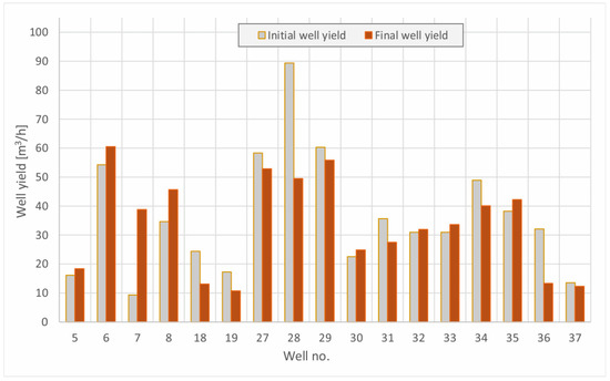
Figure 11.
Initial and final well-yields, porous media.
Well no. 8 is located close to borehole no. 27, the pumping rate of which was estimated correctly and has been stable over years. The same applies to well no. 29. In both cases (no. 27 and 29), only minor ageing-caused changes can be observed.
By analyzing the efficiency curves, it can be concluded that the wells of Group 3 have relatively high efficiencies and critical well-yields at the end of their lifetime. The changes in hydraulic parameters are less significant. These wells have the highest chance of a positive renovation outcome.
These interesting insights provide an analysis of performance parameters. In wells drilled in fractured aquifers, the average critical well-yield amounted to 92.4 m3/h with an average efficiency of 60%. In wells in porous media, the average critical well-yield was only 39.0 m3/h with an efficiency as high as 90%.
It is observed that the average well-yields decrease over time in wells drilled in fractured strata. In Group 1 wells, the average reduction is only 32%, which is associated with a failure of the wells. The average well-yield reduction in Group 2 achieved 62%, and in Group 3, 29%.
In contrast to the above, in wells completed in porous aquifers belonging to Group 1, a 32% well-yield increase was observed. This is the effect of well damage. However, in Groups 2 and 3, there was a well-yield decrease of 43% and 18%, respectively.
6. Conclusions
The method presented in this paper has certain limitations. The basis for the research is the reference step-drawdown test. The reference SDT should be conducted for a single well with a single well-screen that capture one aquifer. Otherwise, a multilevel pumping test is required.
After the completion of the drilling work, the determination of hydrogeological parameters takes place. The pumping test objective is to determine the critical and operational parameters of the well. The reference data allow us to compare the next SDT results and identify a change in direction.
In this study, the efficiency of 40 wells was re-analyzed. Only three of them had an efficiency close to 1.0 (100%). In the remaining 37 cases, incorrectly marked hydrogeological parameters had a negative impact on operational parameters. This could be a result of the premature degradation of the wells.
Due to the ageing of the wells under consideration, the initial parameters have changed. A comparison of the corrected parameters can be used as a basis for inferring the types of physical processes taking place. Determining the hydraulic resistance coefficients in laminar and turbulent flow is a first indication of the degree of filter clogging. To correctly identify the parameters, it is fundamental to establish the course of the well efficiency curve. It is then possible to calculate hydrogeological parameters, e.g., permeability K, conductivity T, or the aquifer penetration ratio b.
After many years of operation, step-drawdown tests were carried out again. Taking efficiency into account, parameters were recalculated, including the well-screen penetration ratio, permeability, and conductivity. This provided a preliminary assessment of the conditions for the continued use of the well.
The results of the research presented in this paper indicate that the most common cause of accelerated degradation and damage to boreholes is overestimating the pumping rate. This causes a high hydraulic gradient and excessive well-loss. In porous strata, damage to the borehole-seal usually occurs. In fractured strata, fine particles are also washed out of the fissure space and the filter becomes clogged. In karstic strata, the aquifer may become unblocked, which sometimes results in an uncontrolled inflow of poor-quality water.
The presented method is suitable for use as a preliminary solution. Since it is non-invasive, it is not cost-intensive. The step-drawdown test can be carried out during a technological break using standard equipment and measurement devices. Additionally, it requires analytical calculations and interpretation of the results achieved.
In the next stages of the work, the results can be further detailed by using invasive investigation methods, such as TV-inspection or geophysical methods. These require the removal of the pumping system and involve higher costs. They involve special technical resources, such as advanced measuring equipment. They are also significantly more time-consuming.
In numerous instances, the method presented in this approach may be sufficient to identify the type of damage and to pre-select repair methods. This is confirmed by the results of subsequent TV-inspections and geophysical surveys, which allowed for detailed identification of the type of clogging and the locations of the damage. However, in cases where only a reduction in filter permeability was identified, geophysical surveys were not necessary to carry out the renovation.
The results of the calculations and analyses presented in this paper confirm the usefulness of the method applied for the preliminary diagnosis of the causes of abnormal well performance. It can be concluded that this method may be useful in technical inspection and repair planning, which are the basic parts of sustainable water resource management.
Author Contributions
Conceptualization, K.P.; methodology, K.P.; software, K.P.; validation, K.P. and K.K.-O.; formal analysis, K.K.-O.; investigation, K.P. and K.K.-O.; data curation, K.P.; writing—original draft preparation, K.P.; writing—review and editing, K.K.-O.; visualization, K.K.-O.; supervision, K.P. All authors have read and agreed to the published version of the manuscript.
Funding
The study has internal support from the Polish Ministry of Science and Higher Education, as part of the subsidy to the AGH University of Science and Technology in Krakow, Faculty of Civil Engineering and Resource Management (no. 16.16.100.215/B500).
Data Availability Statement
The original contributions presented in this study are included in the article. Further inquiries can be directed to the corresponding author.
Acknowledgments
The authors greatly appreciate the helpful and constructive review comments from the anonymous reviewers.
Conflicts of Interest
The authors declare no conflicts of interest.
References
- Walton, W.C. Selected analytical methods for well and aquifer evaluation. In Bulletin Illinois State Water Survey; Illinois State Water Survey: Champaign, IL, USA, 1962; Volume 49. [Google Scholar]
- Bierschenk, W.H. Determining well efficiency by multiple step-drawdown tests. In International Association of Scientific Hydrology Publication; International Association of Scientific Hydrology: Wallingford, UK, 1963; pp. 493–507. [Google Scholar]
- Kurtulus, B.; Yaylım, T.N.; Avşar, O.; Kulac, H.F.; Razack, M. The Well Efficiency Criteria Revisited—Development of a General Well Efficiency Criteria (GWEC) Based on Rorabaugh’s Model. Water 2019, 11, 1784. [Google Scholar] [CrossRef]
- Houben, G.J. The influence of well hydraulics on the spatial distribution of well incrustations. Ground Water 2006, 44, 668–675. [Google Scholar] [CrossRef]
- Henry, J.; Ramey, J.R. Well-Loss Function and the Skin Effect: A Review. In Recent Trends in Hydrogeology; Narasimhan, T.N., Ed.; Geological Society of America: Boulder, CO, USA, 1982. [Google Scholar]
- van Beek, C.G.E.M.; Breedveld, R.J.M.; Juhász-Holterman, M.; Oosterhof, A.; Stuyfzand, P.J. Cause and prevention of well bore clogging by particles. Hydrogeol. J. 2009, 17, 1877–1886. [Google Scholar] [CrossRef]
- Van Beek, K.; Breedveld, R.; Stuyfzand, P. Preventing two types of well clogging. J.-Am. Water Work. Assoc. 2009, 101, 125–134. [Google Scholar] [CrossRef]
- Houben, G.J. Hydraulics of water wells—Head losses of individual components. Hydrogeol. J. 2015, 23, 1659–1675. [Google Scholar] [CrossRef]
- Lennox, D.H. Analysis of Step-Drawdown Test. J. Hydraul. Div. Proc. Am. Soc. Civ. Eng. 1966, 92, 25–48. [Google Scholar]
- Clark, L. The Analysis and Planning of Step Drawdown Tests. Q. J. Eng. Geol. Hydrogeol. 1977, 10, 125–143. [Google Scholar] [CrossRef]
- Birsoy, Y.K.; Summers, W.K. Determination of aquifer parameters from step tests and intermittent pumping data. Ground Water 1980, 18, 137–146. [Google Scholar] [CrossRef]
- Gupta, A.D. On Analysis of Step-Drawdown Data. Groundwater 1989, 27, 874–881. [Google Scholar] [CrossRef]
- Avci, C.B. Parameter Estimation for Step-Drawdown Tests. Ground Water 1992, 30, 338–342. [Google Scholar] [CrossRef]
- Kawecki, M.W. Meaningful Interpretation of Step-Drawdown Tests. Ground Water 1995, 33, 23–32. [Google Scholar] [CrossRef]
- Shekhar, S. An approach to interpretation of step drawdown tests. Hydrogeol. J. 2006, 14, 1018–1027. [Google Scholar] [CrossRef]
- Barker, J.A.; Herbert, R. Hydraulic tests on well screens. Appl. Hydrogeol. 1992, 92, 7–19. [Google Scholar] [CrossRef]
- Avci, C.B.; Ciftci, E.; Sahin, A.U. Identification of aquifer and well parameters from step-drawdown tests. Hydrogeol. J. 2010, 18, 1591–1601. [Google Scholar] [CrossRef]
- Mawlood, D.K.; Mustafa, J.S. Analyse the Well Losses and Aquifer Losses on the Pumping Test Results. ZANCO J. Pure Appl. Sci. 2016, 28, s61–s67. [Google Scholar]
- Houben, G.J.; Kenrick, M.A.P. Step-drawdown tests: Linear and nonlinear head loss components. Hydrogeol. J. 2022, 30, 1315–1326. [Google Scholar] [CrossRef]
- Mathias, S.A.; Todman, L.C. Step-drawdown tests and the Forchheimer equation. Water Resour. Res. 2010, 46, 4. [Google Scholar] [CrossRef]
- Kruseman, G.P.; de Ridder, N.A. Analysis and Evaluation of Pumping Test Data, 2nd ed.; International Institute for Land Reclamation and Improvement: Wageningen, The Netherlands, 1990; pp. 199–215. ISBN 978-9070754204. [Google Scholar]
- Polak, K.; Klich, J.; Kaznowska-Opala, K. The method of wells’ efficiency estimation. In Proceedings of the IMWA Congress, Aachen, Germany, 4–11 September 2011. [Google Scholar]
- Chen, C.; Tao, Q.; Wen, Z.; Wörman, A.; Jakada, H. Step-drawdown test for identifying aquifer and well loss parameters in a partially penetrating well with irregular (non-linear increasing) pumping rates. J. Hydrol. 2022, 614, 128652. [Google Scholar] [CrossRef]
- Dupuit, J. Études Théoriques et Pratiques sur le Mouvement des Eaux Dans les Canaux Découverts et à Travers les Terrains Perméables, 2nd ed.; Dunot: Paris, France, 1863; p. 304. [Google Scholar]
- Rorabaugh, M.J. Graphical and Theoretical Analysis of Step Drawdown Test of Artesian Well. Proc. Am. Soc. Civ. Eng. 1953, 79, 1–23. [Google Scholar]
- Polak, K.; Górecki, K.; Kaznowska-Opala, K. The dynamics of water wells efficiency reduction and ageing process compensation. Water 2019, 11, 117. [Google Scholar] [CrossRef]
- Jacob, C.E. Drawdown test to determine effective radius of artesian well. Trans. Am. Soc. Civ. Eng. 1947, 112, 1047–1064. [Google Scholar] [CrossRef]
- Labadie, J.W.; Helweg, O.J. Step-drawdown test analysis by computer. Ground Water 1975, 13, 46–52. [Google Scholar] [CrossRef]
- Helweg, O.J. General Solution to the Step-Drawdown Test. Ground Water 1994, 32, 363–366. [Google Scholar] [CrossRef]
- Singh, S.K. Well Loss Estimation: Variable Pumping Replacing Step Drawdown Test. J. Hydraul. Eng. 2002, 128, 343–348. [Google Scholar] [CrossRef]
- Singh, S.K. Identifying Head Loss from Early Drawdowns. J. Irrig. Drain. Eng. 2008, 134, 107–110. [Google Scholar] [CrossRef]
- Forchheimer, P. Hydraulic, 3rd ed.; B. G. Teubner: Leipzig-Berlin, Germany, 1930. (In German) [Google Scholar]
- Hansen, C.V. Description and Evaluation of Selected Methods Used to Delineate Wellhead-Protection Areas around Public-Supply Wells near Mt. Hope, Kansas; USGS Water-Resources Investigations Report 90-4102; U.S. Geological Survey: Denver, CO, USA, 1991. [Google Scholar]
- Bear, J. Hydraulics of Groundwater; McGraw Hill: New York, NY, USA, 1979. [Google Scholar]
- Kyrieleis, W.; Sichardt, W. Grundwasserabsenkung Bei Fundierungsarbeiten; Springer: Berlin/Heidelberg, Germany, 1930. (In German) [Google Scholar]
- Louwyck, A.; Vandenbohede, A.; Libbrecht, D.; Van Camp, M.; Walraevens, K. The Radius of Influence Myth. Water 2022, 14, 149. [Google Scholar] [CrossRef]
- El-Hames, A.S. Development of a simple method for determining the influence radius of a pumping well in steadystate condition. J. Groundw. Sci. Eng. 2019, 8, 97–107. [Google Scholar] [CrossRef]
- Motyka, J.; Wilk, Z. Calculated radius of nonlinear zone around fissured-karstified rocks tapping well. Przegląd Geol. 1984, 32, 90–94. (In Polish) [Google Scholar]
- Atkinson, L.C.; Gale, J.E.; Dudgeon, C.R. New Insight to the Step-Drawdown Test in Fractured-Rocks Aquifers. Appl. Hydrogeol. 1994, 2, 9–18. [Google Scholar] [CrossRef]
- Misstear, B.; Banks, D.; Clark, L. Water Wells & Boreholes; John Wiley and Sons Ltd.: Chichester, UK, 2006. [Google Scholar]
Disclaimer/Publisher’s Note: The statements, opinions and data contained in all publications are solely those of the individual author(s) and contributor(s) and not of MDPI and/or the editor(s). MDPI and/or the editor(s) disclaim responsibility for any injury to people or property resulting from any ideas, methods, instructions or products referred to in the content. |
© 2025 by the authors. Licensee MDPI, Basel, Switzerland. This article is an open access article distributed under the terms and conditions of the Creative Commons Attribution (CC BY) license (https://creativecommons.org/licenses/by/4.0/).