Article

Dual-Objective Pareto Optimization Method of Flapping Hydrofoil Propulsion Performance Based on MLP and Double DQN

by
Jingling Zhang
*,
Xuchen Qiu
,
Wenyu Chen
,
Ertian Hua
and
Yajie Shen
College of Mechanical Engineering, Zhejiang University of Technology, Hangzhou 310023, China
*
Author to whom correspondence should be addressed.
Water 2025, 17(22), 3290; https://doi.org/10.3390/w17223290
Submission received: 24 October 2025 / Revised: 11 November 2025 / Accepted: 14 November 2025 / Published: 18 November 2025

Abstract

To address the inherent complexities of underwater operating environments and achieve the design of a highly efficient, energy-saving flapping hydrofoil, this paper proposes an intelligent agent-based model for real-time parametric optimization. A non-parametric surrogate model based on a Multilayer Perceptron (MLP) is established using data samples of multi-dimensional flapping hydrofoil geometric parameters obtained through Computational Fluid Dynamics (CFD) simulations. An improved Double Deep Q-Network (DDQN) algorithm incorporating Pareto frontier information is deployed within the surrogate model to obtain the Pareto optimal solution set for propulsion efficiency and average input power, and a set of propulsion parameter combinations with error ranges between 0.24% and 1.27% across continuous intervals was obtained. Experimental results demonstrate that the proposed MLP-DDQN method is capable of learning the domain-wide optimal solution within the experimental environment, satisfying the Pareto optimality between propulsion efficiency and average input power. Further analysis of the flow field around the flapping hydrofoil under the obtained optimal parameter combination revealed that the presence of stable and continuously attached vortex structures on the wing surface is the intrinsic mechanism responsible for its superior propulsion performance.

1. Introduction

With the growing demand for marine resource exploration and underwater operations, efficient and flexible underwater propulsion systems have become a key research focus [1]. Compared to propellers [2], flapping hydrofoils have emerged as a major research subject in the design of underwater vehicles due to their excellent fluid adaptability and energy conversion efficiency [3]. As a core propulsion component, the hydrodynamic performance of flapping hydrofoils directly determines the overall system performance. Therefore, investigating the propulsion performance of the flapping hydrofoil and the underlying flow mechanism responsible for the enhanced performance is of great significance for developing efficient underwater propulsion systems [4].
The influence of geometric parameters on hydrodynamic performance has consistently been a focal point of research [5]. Previous studies have demonstrated that specific structural configurations, such as the pitch-axis location and leading-edge shape, are crucial for optimizing key performance metrics, including thrust, power coefficient, and propulsion efficiency [6]. Zhao et al. [7] investigated the propulsion performance of NACA 0015, examining the influence of pivotal factors such as the pivot position, maximum thickness, and maximum angle of attack on its hydrodynamic performance. Their study determined that specific structural configurations of the flapping hydrofoil can effectively enhance its cavitation resistance and reduce flow field instability. Zhang et al. [8] conducted a study on the hydrodynamic performance of a three-dimensional flapping hydrofoil, simulating the flow field variations in NACA 0012 under different parameters, including aspect ratios, tip ratios, and forward-swept and back-swept shapes. Through comparative analysis, they identified optimized geometric design parameters for the flapping hydrofoil structure. Gupta et al. [9] demonstrated that the hydrodynamic performance and stability of flapping hydrofoils improve with reduced relative thickness and increased curvature of the leading and trailing edge. Guo et al. [10] conducted hydrodynamic model experiments on a three-dimensional flapping hydrofoil with different leading-edge configurations, investigating their hydrodynamic performance under various oscillating frequencies and analyzing the influence of different leading-edge structures on hydrofoil performance. Zhe et al. [11] introduced vortex-generator (VG) flow-control concepts into tidal-turbine blade design and used CFD to examine how geometric parameters of VGs affect the hydrodynamic performance of NACA 4418.
In recent years, with the rapid development of intelligent optimization algorithms and machine learning technologies, there has been an increasing number of studies focused on integrating these technologies with the optimization of flapping hydrofoil hydrodynamic performance [12]. Song et al. [13] employed an integrated approach combining the Taguchi experimental, neural networks, and CFD to systematically investigate the influence of parameters, including aspect ratio, heaving amplitude, pitching amplitude, and flapping frequency, on the propulsion performance of a three-dimensional NACA 0012. Najafi et al. [14] utilized an artificial neural network (ANN) to predict key performance parameters under different Froude numbers (Fr) and hydrofoil types, with the aim of identifying suitable hydrofoils between two hulls of catamarans. Wang [15] proposed a novel static fluid-structure interaction (FSI) tool based on deep learning, which efficiently solves the FSI problem and demonstrates its capability in accurately predicting the elastic deformation of a flexible hydrofoil. Yang et al. [16] constructed a non-parametric model generalizing across operational environments based on a Gaussian Process Regression (GPR) algorithm and employed Deep Reinforcement Learning (DRL) to acquire the globally optimal combination of motion parameters for flapping hydrofoil propulsion within the entire defined domain under experimental conditions. Kostas et al. [17] developed an optimization framework based on an isogeometric boundary element method (BEM) potential flow solver for hydrofoil geometric parameter optimization.
Although the CFD simulation provides high accuracy in analyzing the hydrodynamic performance of the flapping hydrofoil under various parametric conditions, extensive simulation experiments are highly time-consuming [18]. Furthermore, no definitive correlation has been established between the hydrodynamic performance and geometric parameters, such as the pitch-axis location and curvature [19]. Therefore, rapidly identifying the coupled geometric parameters that correspond to optimal hydrodynamic performance within a defined domain holds significant research value.
To establish an accurate model for flapping hydrofoil motion and account for the strongly nonlinear effects of the underwater environment, this paper employs the MLP for nonlinear modeling of flapping hydrofoil propulsion. Concurrently, the DDQN is used to enable autonomous optimization through the interaction between the underwater flapping hydrofoil and its environment. This paper proposes an MLP-DDQN collaborative optimization method, which utilizes the MLP to construct a flapping hydrofoil surrogate model and incorporates the DDQN algorithm to efficiently identify optimal geometric parameters that maximize propulsion performance and meet specific performance requirements, even under small-sample conditions. This approach offers an efficient and reliable solution for the intelligent design of underwater propulsion systems.

2. Flapping Hydrofoil Propulsion Problem

As the core actuating component of the underwater propulsion system, the geometric features of the flapping hydrofoil directly influence its hydrodynamic performance. The NACA four-digit series airfoils, developed by the U.S. National Advisory Committee for Aeronautics (NACA), are widely used in such research due to their parametric design specifications and extensive experimental data [20]. Therefore, this paper selects the NACA four-digit series as the baseline model for the two-dimensional hydrofoil. Taking the NACA 4418 as an example, its profile and key geometric parameters are illustrated in Figure 1.
By dividing the maximum thickness t, maximum camber f, location of maximum camber x f , and from Figure 1 by the chord length c, their corresponding dimensionless parameters are obtained: namely, relative thickness t * = t / c , relative camber f * = f / c , and location of relative camber x f * = x f / c . The pitch-axis location is defined as x p * = x p / c .
The motion of the flapping hydrofoil primarily consists of coupled heave and pitch, and is governed by the following equations of motion [21]:
y ( t ) = y ( 0 ) sin ( ω t )
θ ( t ) = θ ( 0 ) sin ( ω t + ϕ )
where y ( t ) is the heave displacement of the flapping hydrofoil, θ ( t ) is the pitch angle of the flapping hydrofoil, y ( 0 ) and θ ( 0 ) are their amplitudes, and ϕ is the phase lag between heave and pitch motion.
In the study of the flapping hydrofoil, the instantaneous thrust coefficient C T ( t ) and instantaneous lift coefficient C L ( t ) are key metrics for evaluating the hydrodynamic performance of the flapping hydrofoil, and are defined as follows:
C T ( t ) = F x ( t ) 1 2 ρ U 2 c s
C L ( t ) = F y ( t ) 1 2 ρ U 2 c s
where F x ( t ) is the instantaneous thrust in the horizontal direction, F y ( t ) is the instantaneous thrust in the vertical direction, ρ is the fluid density, U 2 is the mean incoming velocity, and s is the span length.
Over one flapping period, the mean thrust coefficient C T ¯ and mean lift power C L ¯ are defined as follows:
C T ¯ = 1 T t t + T C T ( t ) d t
C L ¯ = 1 T t t + T C L ( t ) d t
This paper addresses the optimization of propulsion performance for the flapping hydrofoil with respect to a set of geometric parameters, denoted as [ x p * , t * , x f * , f * ]. The symbols and admissible ranges of these parameters are summarized in Table 1. We adopt the averaged input power P in ¯ and the propulsion efficiency η as the propulsion performance metrics.
The mean power coefficient C P ¯ is defined as follows:
C P ¯ = 1 T t t + T C P ( t ) d t = 2 P in ¯ ρ U 3 c
where C P ( t ) is the instantaneous power coefficient, and P in ¯ reflects the energy consumption of the flapping hydrofoil motion, which is defined as follows:
P in ¯ = 1 T t t + T F y ( t ) y ˙ ( t ) + M ( t ) θ ˙ ( t ) d t
where M ( t ) is the instantaneous torque of the flapping hydrofoil around the center of rotation.
Ultimately, the propulsion efficiency η quantifies the capability of the flapping hydrofoil to convert input energy into propulsive power, which is defined as follows:
η = C T ¯ C P ¯

3. Numerical Method

3.1. Control Equations and Turbulence Modeling

During flapping, vortices are repeatedly generated and shed from the hydrofoil surface, requiring accurate resolution of near-wall boundary-layer dynamics. The Reynolds time-averaged Navier–Stokes (RANS) method is well suited to capturing boundary-layer separation and reattachment with relatively modest mesh requirements and exhibits robust convergence in iterative solvers. Therefore, this paper employs the Reynolds time-averaged Navier–Stokes (RANS) equations to capture the two-dimensional incompressible turbulent flow field. The governing equations for the flow motion are as follows [22]:
u ¯ i x i = 0 , i = 1 , 2
u ¯ i t + u ¯ j u ¯ i x j = 1 ρ p ¯ x i + x j γ + γ t u ¯ i x j + u ¯ j x i
where u ¯ i denotes the fluid velocity components; x i represents the control coordinates; p is the fluid pressure; t denotes the time; γ is the kinematic viscosity; γ t = c μ k 2 / ε is the turbulent viscosity coefficient (with c μ represents the model constant); k stand for the turbulent kinetic energy; and ε is the turbulent dissipation rate.
To more accurately capture the complex characteristics of such flow fields, the realizable k- ε turbulence model was employed in this study to solve the above Reynolds time-averaged Navier–Stokes (N-S) equations; the corresponding literature can be found in [23].

3.2. Computational Domain and Meshing

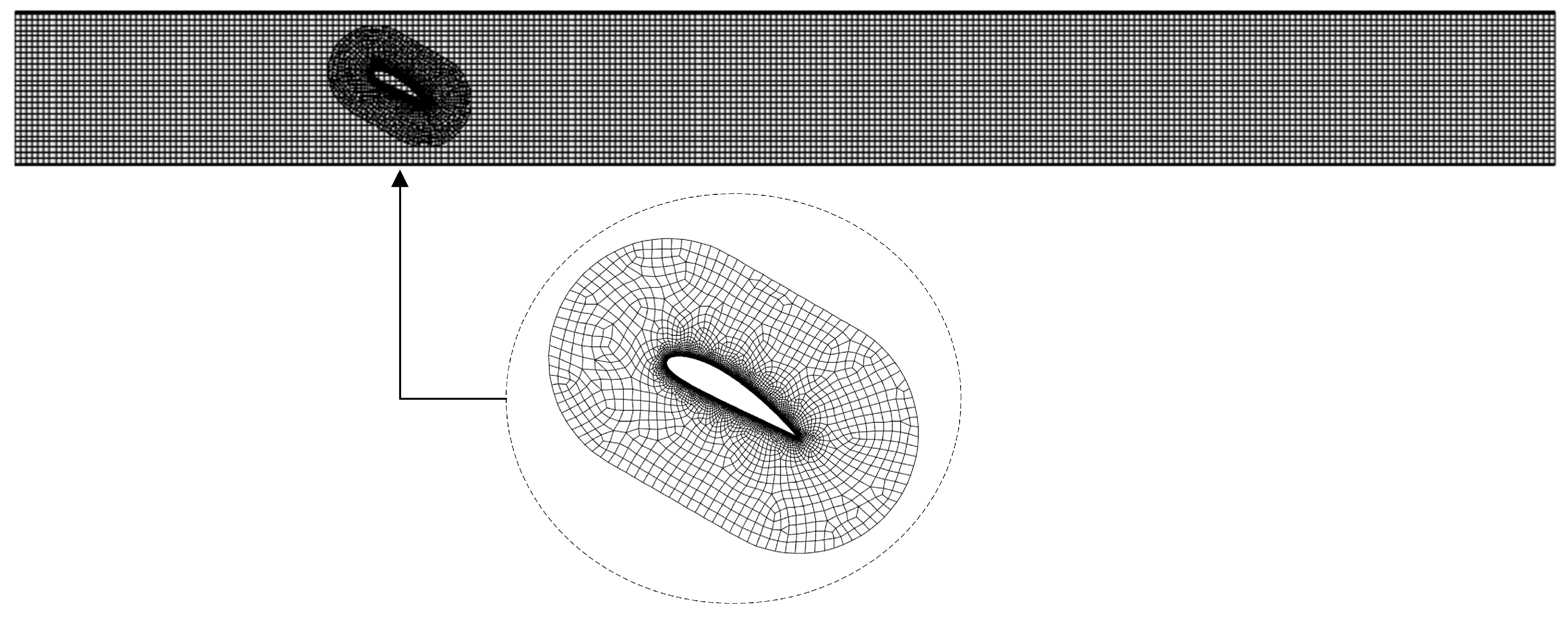
The size of the computational domain and the influence of far-field boundary conditions cannot be neglected. To ensure full wake development around the hydrofoil, the downstream extent is commonly set to 20 c , where c denotes the chord length. In this study, the total length in the x-direction is 8 m , with 6 m extending in the positive x-direction, and the hydrofoil is centered at the origin. To emulate the effect of channel banks relevant to riverine propulsion, the channel width is set to 0.9 m . The grid division of the computational domain is shown in Figure 2.
To capture the transient flow during hydrofoil motion, dynamic meshing was performed using an overset-grid approach. An elliptical deforming subdomain centered on the pitch axis was discretized with an unstructured quadrilateral mesh, while the remainder of the domain employed a structured grid. To better resolve the near-wall boundary layer along the hydrofoil and solid walls, a prismatic inflation layer was applied with a first-layer height of 0.0572 mm , a growth rate of 1.2 , and 15 layers in total.
To assess grid independence, simulations were performed on meshes of three densities: 2.25 × 10 4 (coarse), 3.6 × 10 4 (medium), and 7.2 × 10 4 (fine) cells. The results are shown in Figure 3. The temporal evolution of the instantaneous thrust coefficient obtained with the medium and fine meshes exhibits close agreement, indicating that further refinement has a negligible effect on the solution. Therefore, to balance accuracy and computational cost, the medium mesh is adopted for subsequent simulations.

3.3. Numerical Method Validation

Numerical simulations of hydrofoil propulsion were performed in Ansys Fluent 2022R1 using the realizable k- ε turbulence model and an overset-grid technique. A pressure-inlet boundary condition was prescribed at the domain entrance to represent quiescent water, and a pressure-outlet was applied at the exit. The hydrofoil surface and channel banks were modeled as stationary walls. Hydrofoil motion was imposed via a user-defined function (UDF). Pressure–velocity coupling employed the coupled algorithm and spatial discretization used the second-order upwind scheme. The time step was chosen to be smaller than the ratio of the minimum grid size to the characteristic flow speed and was adaptively adjusted during the computation to maintain numerical stability.
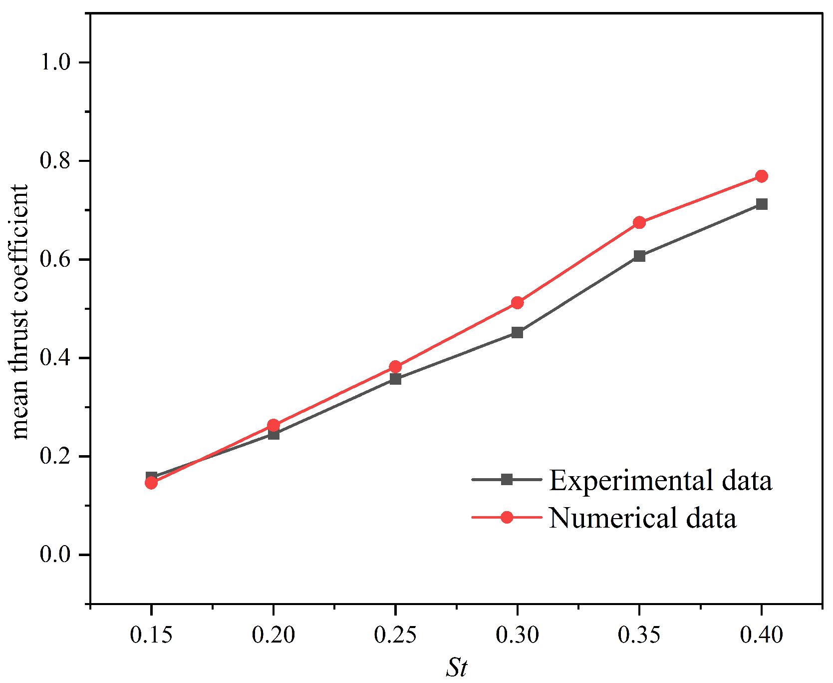
To verify the reliability of the numerical methodology, according to the experimental study on the propulsive performance of flapping hydrofoils in the literature [24], a corresponding simulation model is established to evaluate the propulsion performance of the flapping hydrofoil. The numerical method employed herein is validated by comparison with the experimental results reported in [24], with the computational model and simulation parameters matched to the experimental conditions in that study: the chord length c = 0.1 m ; the mean incoming velocity U 2 is taken as 0.4 m / s ; the phase difference ϕ = 90 ; the heave amplitudes y 0 = 0.075 m ; the maximum angle of attack α max = 20 ; the Reynolds number R e = 4.0 × 10 4 .
Figure 4 shows that the numerical calculation results in this paper are consistent with the experimental results and exhibit the same trends, confirming the effectiveness of the adopted numerical method.

4. Methodology

4.1. Overview of MLP-DDQN Framework

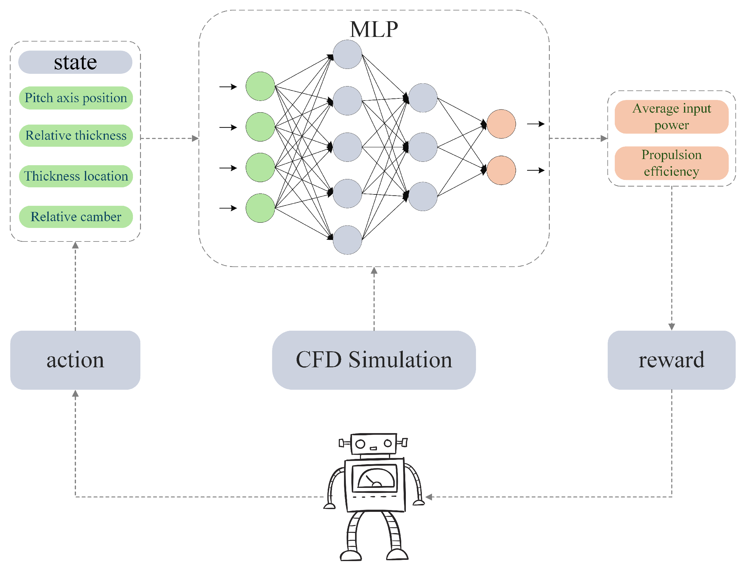
Although traditional CFD simulations accurately resolve flow fields, vortex evolution, and hydrodynamic loads of the flapping hydrofoil, their high computational cost makes them impractical for large-scale, iterative, parametric optimization. Moreover, deep reinforcement learning (DRL) methods that rely on online interaction with such high-cost simulators suffer from prohibitive sample complexity. To address these challenges, we propose a collaborative optimization framework, the MLP-DDQN method, which couples an MLP surrogate model with an enhanced DDQN augmented by Pareto-front information. The MLP efficiently learns the nonlinear mapping from geometric-parameter space to performance metrics, yielding a high-fidelity, low-cost surrogate that replaces the original CFD environment. This surrogate enables rapid prediction of key performance metrics for candidate parameter sets and provides real-time environment feedback to the RL agent. Guided by Pareto-front information, the agent performs dual-objective optimization of propulsion efficiency and averaged input power.
The core workflow comprises three phases: (i) systematic sampling of hydrodynamic performance under different hydrofoil configurations via parameterized CFD simulations; (ii) training an MLP-based surrogate model to learn the nonlinear mapping from geometric parameter combinations to propulsion metrics; and (iii) deploying an improved DDQN algorithm within the surrogate environment to perform global optimization over the geometric design space. The proposed MLP–DDQN framework is illustrated in Figure 5. In this framework, the MLP-based surrogate acts as a compact model of the hydrodynamic environment, mapping each geometric state to the corresponding averaged input power P in and propulsive efficiency η , from which the reinforcement-learning reward is computed. The agent’s observed state is a normalized geometric parameter vector s t = [ x p * , t * , x f * , f * ] representing the current hydrofoil configuration. A 12-dimensional discrete action space is adopted, where each action perturbs one or several components of s t by a prescribed step size.

4.2. MLP for Hydrofoil Parameter-Performance Mapping

4.2.1. Introduction to MLP Model

The Multilayer Perceptron (MLP) is a feedforward neural network comprising an input layer, one or more hidden layers, and an output layer, each consisting of multiple neurons [25,26,27,28]. The input layer receives external signals and passes them to the first hidden layer; thereafter, each layer takes the previous layer’s outputs as inputs, applies an affine transformation with learnable weights W and biases b , and then a nonlinear activation to produce its output.
Given a training dataset of N samples { ( x i , y i ) } i = 1 N , the MLP defines via layer-wise forward propagation a nonlinear mapping f θ : X Y with parameters θ = { W , b } . For each sample, the network is trained to minimize the discrepancy between predictions y ^ i = f θ ( x i ) and ground-truth labels y i , measured by a regression loss function ( y ^ i , y i ) that is differentiable with respect to the network parameters θ . Gradients of L ( θ ) with respect to θ are computed by backpropagation and used by a gradient-based optimizer to update the network parameters. Accordingly, the empirical risk minimization objective is
min L ( θ ) = 1 N i = 1 N y ^ i , y i .

4.2.2. MLP Architecture and Training

For geometric parameter combinations, the MLP accurately captures the complex mapping relationships between geometric parameters and propulsion performance metrics through nonlinear transformations in its hidden layers, thereby providing efficient environmental feedback for reinforcement learning agents.
This paper constructs a data-driven MLP surrogate with three hidden layers: the input layer takes a four-dimensional feature vector; the hidden layers contain 128, 64, and 32 neurons, respectively; and the output layer produces a single performance prediction. To improve training stability, a residual connection projects the input directly to the third hidden layer, alleviating vanishing-gradient effects. Batch-normalization layers are included to reduce overfitting and enhance generalization. During training, we optimize the Huber loss to improve robustness to noisy targets, and use the AdamW optimizer with an initial learning rate of 0.001, together with a learning-rate scheduler to accelerate convergence and avoid poor local minima.

4.3. DDQN Incorporating Pareto Frontier Information

4.3.1. Introduction to Deep Reinforcement Learning

Deep reinforcement learning (DRL) integrates deep neural networks with the reinforcement-learning framework to learn decision policies through continual interaction between an agent and its environment [29,30,31,32]. The decision-making problem is modeled as a Markov decision process (MDP) S , A , P , R , γ , where S is the state space (the agent observes s t S ), A is the action space (the agent selects a t A according to a policy π ( a | s ) ), P ( s t + 1 s t , a t ) denotes the state-transition probability, R ( s t , a t ) is the reward function, and γ [ 0 , 1 ] is the discount factor. At each discrete time step t, the agent observes the current state s t , samples an action a t π ( · | s t ) , and upon executing a t receives a scalar reward r t = R ( s t , a t ) together with the next state s t + 1 . This interaction generates experience tuples ( s t , a t , r t , s t + 1 ) , which are used to update the parameters of the decision policy or value function. The objective of DRL is to learn a policy that maximizes the expected cumulative discounted return:
G t = k = 0 γ k r t + k .

4.3.2. DDQN for Hydrofoil Optimization

This paper proposes an improved DDQN algorithm that embeds Pareto-front information into the training process. The detailed workflow is summarized in Algorithm 1. To handle the two propulsion objectives—averaged input power P in and propulsive efficiency η , we first construct a coarse approximation of the Pareto front in the objective space using the MLP surrogate. Specifically, the surrogate is evaluated on a set of representative geometric designs, and the corresponding pairs ( P in , η ) are filtered by non-domination to obtain an archive F 0 of Pareto-optimal candidates. From this archive, we identify an engineeringly acceptable region in the objective space and define two thresholds: a maximum admissible power τ p and a minimum acceptable efficiency τ e .
Algorithm 1 DDQN with Pareto Optimization
Require: 
Hydrofoil design parameters P , constraint function C , performance models f P in ¯ , f η , Pareto thresholds τ p , τ e
1:
Initialize replay buffer D , online network Q θ , target network Q θ
2:
for episode = 1 , 2 , , E  do
3:
      Sample initial design s 0 P
4:
      for  t = 0 , 1 , , T max  do
5:
            Select action a t via ϵ -greedy policy from Q θ ( s t )
6:
            Execute a t , observe s t + 1 , and predict:
7:
                 P in ¯ f P in ¯ ( s t + 1 ) , η f η ( s t + 1 )
8:
            Compute reward with Pareto bonus:
9:
                 r t ( η × 100 P in ¯ / 10 ) + β · I [ P in ¯ < τ p η > τ e ]
10:
            Store transition ( s t , a t , r t , s t + 1 ) in D
11:
            Standard DDQN Update:
12:
                Sample minibatch B D
13:
                Compute target y j = r j + γ Q θ ( s j + 1 , arg max a Q θ ( s j + 1 , a ) )
14:
                Update θ via gradient descent on 1 | B | ( y j Q θ ( s j , a j ) ) 2
15:
                Soft update: θ τ θ + ( 1 τ ) θ
16:
      end for
17:
      Pareto Front Analysis:
18:
      for all valid designs s P  do
19:
            if  f P in ¯ ( s ) < τ p f η ( s ) > τ e  then
20:
                 Update Pareto front F F { ( s , f P in ¯ ( s ) , f η ( s ) ) }
21:
            end if
22:
      end for
23:
      Save F
24:
end for
Within the DDQN framework, the current state s t is the normalized geometric parameter vector, and the agent selects an action a t that updates the design to s t + 1 . After querying the MLP surrogate for the corresponding performance metrics O P = P in ( s t + 1 ) and O η = η ( s t + 1 ) , the reward is decomposed into a base scalarization term and a Pareto-aware bonus.
The base reward linearly combines the two objectives as follows:
R b = 100 O η 1 10 O P
where R b measures the trade-off between propulsive efficiency and averaged input power for the updated design.
The Pareto-front bonus incorporates the threshold information and is defined as follows:
R p = β I P in ( s t + 1 ) < τ p η ( s t + 1 ) > τ e
where β > 0 is a bonus coefficient and I [ · ] denotes the indicator function.
In conclusion, the total reward at time step t is then given by the following:
R t = R b + R p
This study employs the DDQN architecture with a learning rate of 1 × 10 4 to reduce training oscillations and mitigate divergence. Exploration follows an ε -greedy policy: the initial exploration rate is set to 0.9 to ensure sufficient random exploration in early training, and is linearly annealed to 0.1 to gradually shift toward experience-driven exploitation, thereby balancing exploration and exploitation.

4.3.3. MLP-DDQN for the Fluid Solver

Although DRL can, in principle, train directly within flapping hydrofoil propulsion simulators to discover optimal parameter combinations, its practical deployment is hindered by prohibitive cost. Each CFD evaluation for a hydrofoil propulsion case may require hours, while effective DRL training typically demands thousands of samples, leading to extreme cumulative compute and wall time. Consequently, applying DRL for end-to-end parameter optimization poses substantial engineering feasibility challenges.
In this paper, we introduce an MLP surrogate to learn the mapping from hydrofoil geometry to propulsion performance, and employ an improved DDQN algorithm for optimization on the surrogate. To realize cooperative dual-objective optimization, we incorporate Pareto-front information to refine the solution set. A database linking geometric parameters to hydrodynamic responses is constructed via CFD, and the MLP is trained to approximate the mapping from the geometric parameter combinations to performance metrics. Within the DDQN framework, the agent’s observed state is a normalized vector of hydrofoil parameters, and the objective is to identify Pareto-optimal trade-offs between propulsion efficiency η and averaged input power P in ¯ . The agent conducts autonomous policy search guided by a reward shaping term that biases exploration toward the Pareto front, thereby achieving coordinated improvement in both efficiency and power consumption.

5. Results and Discussion

In this paper, we employ a two-dimensional rigid flapping hydrofoil. Apart from the geometric parameters to be optimized, the following motion parameters are fixed: chord length c = 0.3 m ; flapping frequency f = 1 Hz ; angular frequency ω = 2 π rad s 1 ; heave amplitude y ( 0 ) = 0.5 c ; pitch amplitude θ ( 0 ) = 30 .
All experiments are performed on an Intel Core i5–14600KF CPU @ 3.50 GHz with 32 GB RAM running Windows 11. The code is implemented in Python (version 3.11.5).

5.1. MLP Surrogate Model

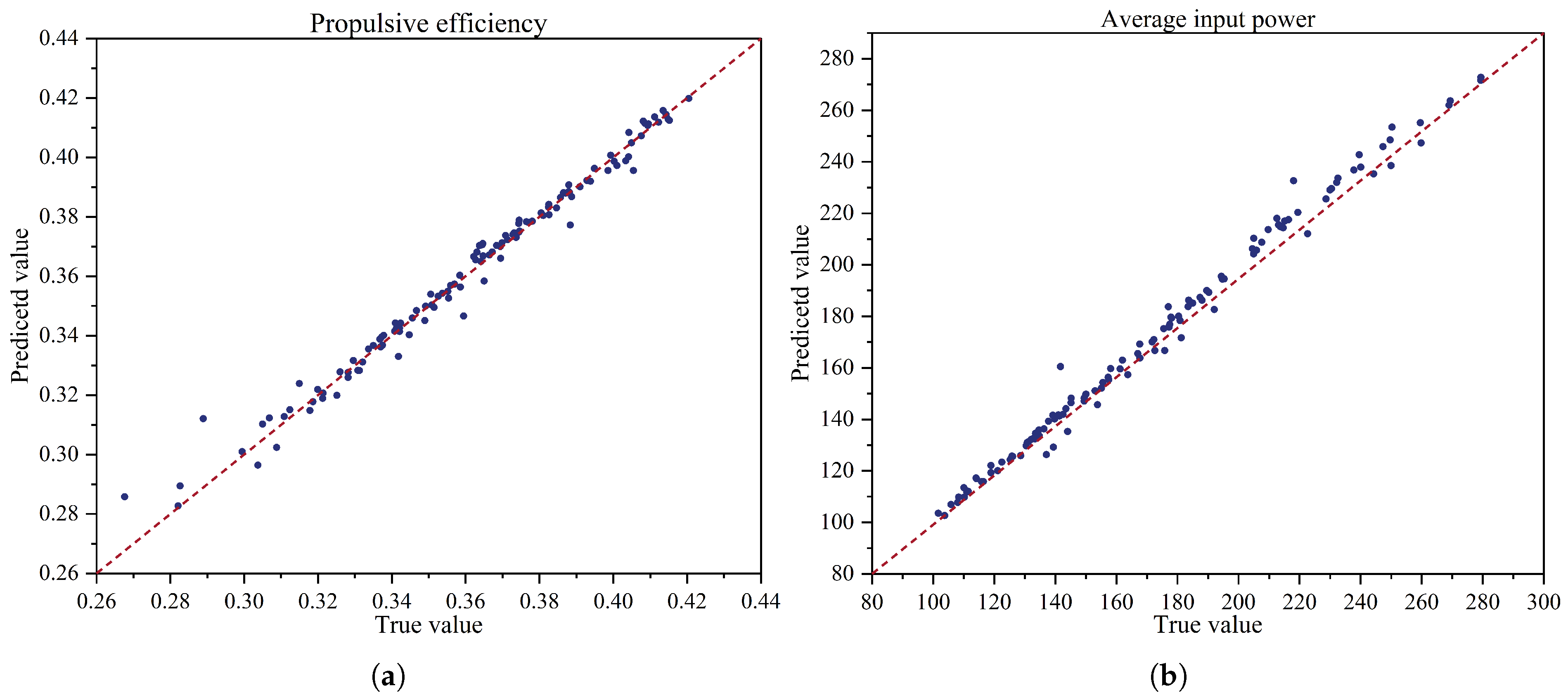
A non-parametric MLP surrogate is constructed to map geometric parameters to propulsion performance metrics. The dataset is generated via CFD simulations, with the flapping-hydrofoil geometric parameters serving as input features and the averaged input power and propulsive efficiency as targets. In total, 624 samples are collected over the design space, and the dataset is randomly split in an 8:2 ratio into a training set and a validation set. During training, the network parameters are optimized using adaptive gradient-based methods with appropriate regularization to enhance generalization and stabilize convergence. The evolution of the training and validation losses exhibits similar decreasing trends and eventually stabilizes at comparably low values, indicating that the surrogate does not suffer from severe overfitting. Parity plots of MLP predictions versus ground truth on the validation set are shown in Figure 6.
In Figure 6a, the MLP surrogate exhibits strong predictive performance on the validation set for propulsive efficiency: the scatter points cluster tightly about the reference line ( y = x ). As shown in Figure 6b, the predictions for averaged input power are similarly accurate. Although a few outliers appear, they constitute less than 2 % of all samples. Overall, more than 95 % of predictions fall within an acceptable error range, indicating that the model effectively captures the nonlinear mapping between airfoil geometry and propulsion performance. The detailed performance metrics of the MLP surrogate are reported in Table 2.
In terms of predictive accuracy, the surrogate exhibits consistently high performance on both the training and validation sets. For averaged input power, the validation coefficient of determination reaches R 2 = 0.9944 , with the corresponding MAE remaining below 2.0 , indicating only small deviations over the explored power range. Propulsive efficiency is predicted with similarly high accuracy, achieving a validation R 2 = 0.9819 and MAE on the order of 10 3 . In both cases, the training errors are only marginally lower than the validation errors, suggesting that the surrogate captures the nonlinear dependence on hydrofoil geometry without noticeable overfitting. Regarding computational efficiency, a single forward pass of the surrogate requires only 0.25–0.27 ms, providing several orders of magnitude speedup over the original CFD simulations, which take on the order of hours per evaluation. Consequently, the MLP surrogate can provide accurate and timely environment feedback for the RL agent, thereby enabling the subsequent dual-objective optimization.

5.2. DDQN Agent

During training, the agent’s observed state is a normalized geometric parameter vector [ x p * , t * , x f * , f * ] . The optimization objective is to identify Pareto-optimal solutions that balance propulsive efficiency and averaged input power. A 12-dimensional discrete action space is adopted, supporting both independent parameter updates and coordinated multivariable adjustments. To bias the search toward practically attractive designs, we introduce two scalar thresholds in the reward: a maximum admissible input power τ p = 140 W and a minimum acceptable efficiency τ e = 38 % . These values are chosen based on a preliminary surrogate-based Pareto analysis of the CFD database (Section 4.2 and Figure 7), in which they correspond to a knee region of the Pareto front. Within the DDQN reward, ( τ p , τ e ) are implemented as soft preference parameters: an additional bonus is issued whenever a candidate simultaneously satisfies the power and efficiency constraints.
Figure 8 shows the DDQN training curves: the averaged reward (right axis) and the Q-network loss (left axis) versus training steps. The loss L Q denotes the standard DQN value-function loss, i.e., MSE between the current Q-network predictions and the bootstrapped target values. The initial stage exhibits pronounced loss oscillations, reflecting exploratory behavior in the design space; this is followed by a rapid convergence phase, during which the agent discovers high-quality regions and the loss drops sharply. Subsequently, the process stabilizes, with the loss fluctuating around 0.7 , indicating that the agent approaches the global Pareto optimum while local optima remain in the landscape.
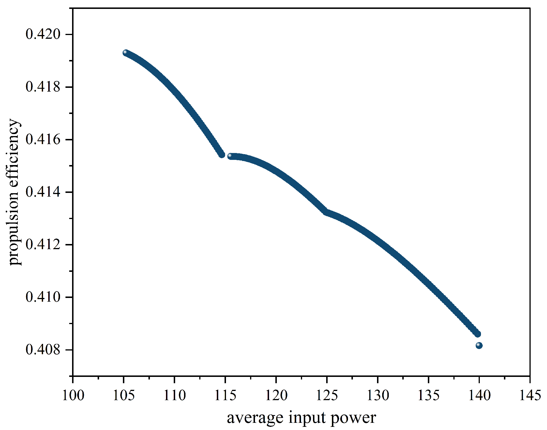
The Pareto-front scatter obtained by the DDQN during parameter optimization is shown in Figure 7, with the abscissa denoting averaged input power and the ordinate propulsive efficiency. A local-optimum region is observed for powers of 115–124 W. In this interval, efficiency growth slows and, at times, both power and efficiency decline simultaneously, indicating that the agent becomes trapped in a parameter-space basin without yielding non-dominated improvements. By contrast, the non-dominated set outside this range is more uniformly distributed. For averaged input powers of 103–113 W, efficiency rises rapidly, indicating that the agent has discovered an optimal combination—rearward maximum-camber location, moderate camber, and an optimized pitch-axis position—thereby approaching the optimal solution.
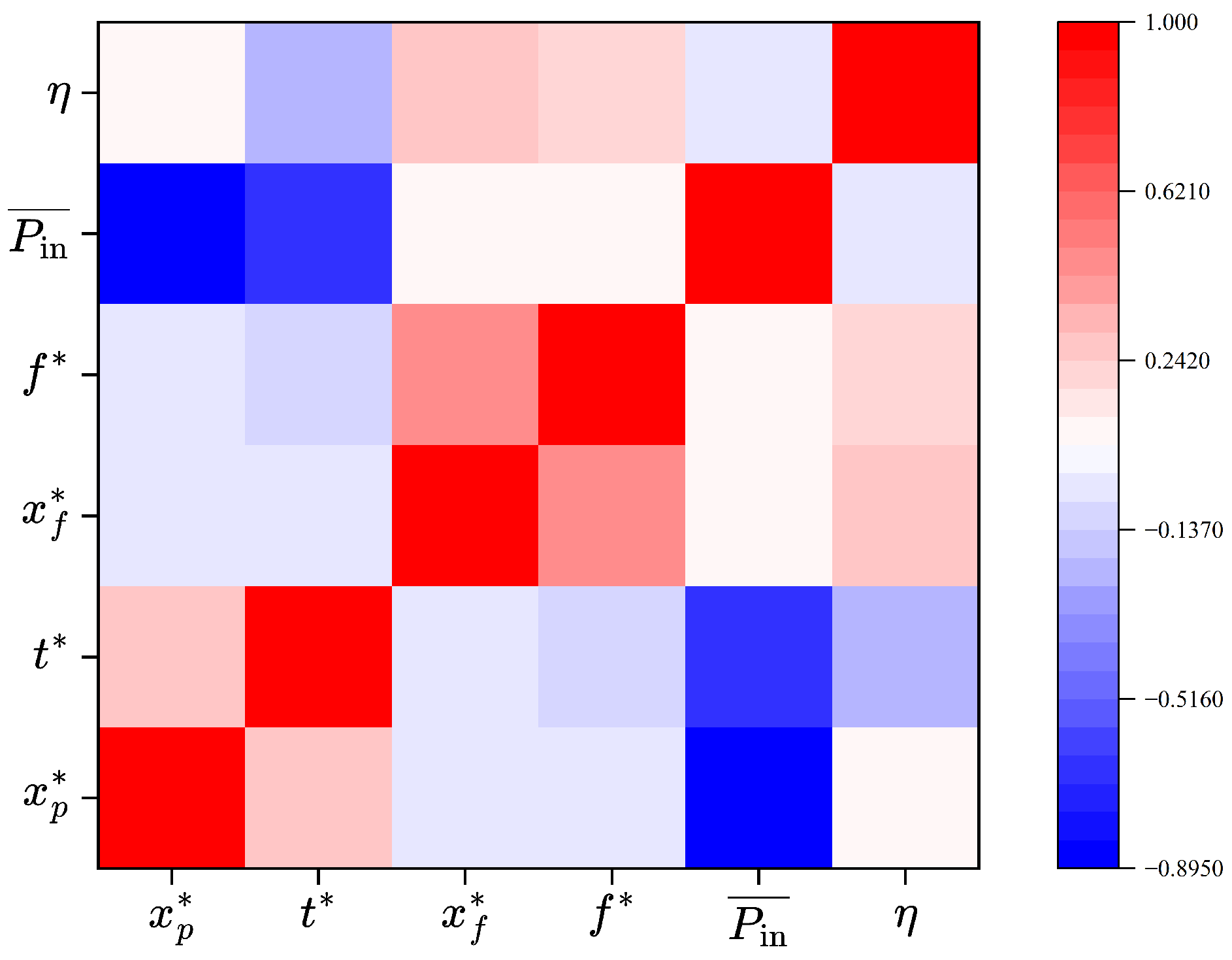
The heatmap analysis of parameter distributions within the Pareto set is shown in Figure 9. The pitch-axis location and relative thickness exhibit strong negative correlations with averaged input power (correlation coefficients 0.895 and 0.516 , respectively), indicating that, within the studied range, appropriately increasing these variables can effectively reduce the required power. By contrast, relative camber and the chordwise location of maximum camber correlate positively with propulsive efficiency (coefficients 0.621 and 0.242 , respectively), suggesting that a leading-edge geometry with moderate camber and a rearward relative camber position enhances propulsive efficiency. Overall, attaining Pareto optimality in both average input power and efficiency necessitates the joint optimization of the leading-edge shape and the pitch-axis location, thereby balancing low power consumption with high propulsion performance.
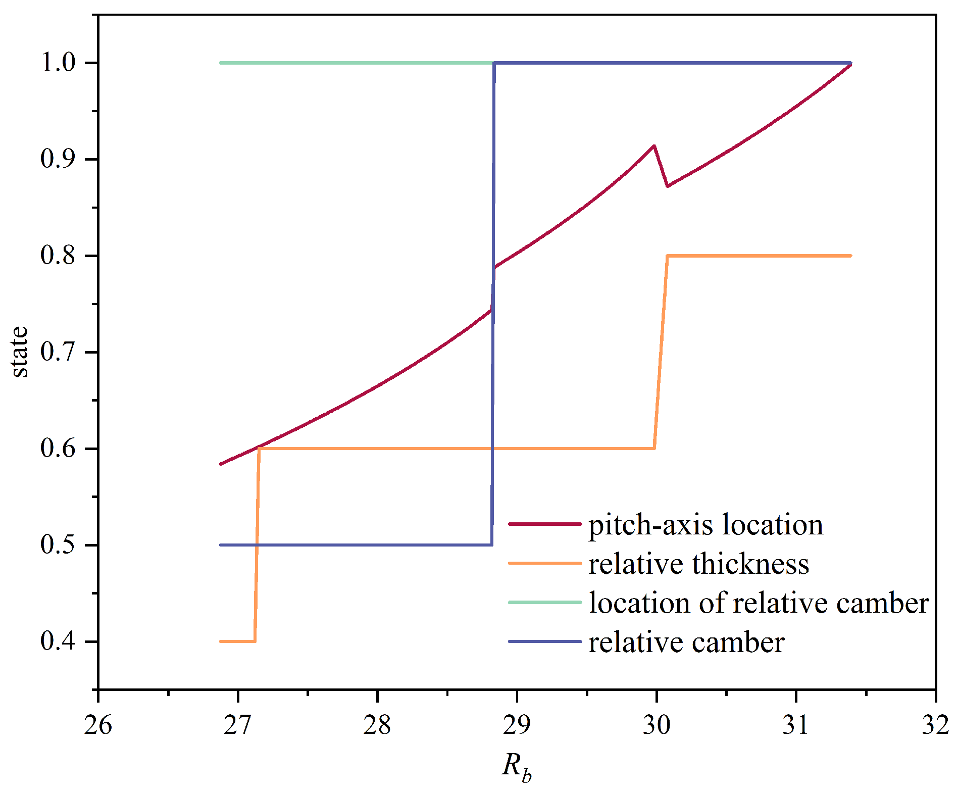
The evolution of normalized state variables for the Pareto-front solutions is shown in Figure 10, with all states scaled to [ 0 , 1 ] . As the base reward rises from its initial level to the peak, the parameters exhibit pronounced co-evolution. The pitch-axis location drifts continuously rearward from an initial normalized value of 0.58 (i.e., 29.2 % chord), while the relative thickness follows a three-stage trajectory and ultimately reaches 0.8 , corresponding to an actual relative thickness of 18 % . The DDQN uncovers multiple local optima; in particular, a thin leading edge combined with high camber produces negative coupling that reduces efficiency. The agent then converges toward the optimum, with the peak reward attained at the geometric parameter vector [ 0.996 , 0.8 , 1.0 , 1.0 ] , representing the physical state [ 49.8 , 18 , 4 , 4 ] (in the units defined for pitch-axis location, relative thickness, relative camber location, and relative camber, respectively). The resulting optimum aligns well with the local-optimum region inferred from the MLP surrogate, indicating satisfactory convergence and generalization when using an MLP-based environment model.
The trained model was then used to perform global optimization of parameter combinations over the design space. By adjusting the reward function, efficiency-maximizing designs were obtained under different averaged input-power constraints. Table 3 summarizes four representative Pareto-front solutions: the unconstrained algorithmic optimum and three constrained cases with power caps of 120, 130, and 140 W , which correspond to practical design scenarios with different available input-power budgets. For each case, the table reports the best propulsive efficiency achieved under the specified power limit, together with the corresponding CFD evaluations and MLP–DDQN predictions for the averaged input power P in and propulsive efficiency η . The relative errors in both P in and η across these four Pareto solutions lie between 0.24 % and 1.27 % , demonstrating the high fidelity of the MLP–DDQN predictions with respect to the CFD evaluations. Compared with training DDQN directly in the CFD environment (which requires thousands of samples [16]), the MLP–DDQN method uses only about 14.5 % of the sample count, yielding markedly higher efficiency. These results indicate that the MLP–DDQN method preserves optimization effectiveness while substantially improving RL training efficiency and reducing computational cost.

5.3. Influence of the Parameter Combinations on the Propulsive Performance

To investigate the intrinsic mechanisms by which parameter combinations affect flapping hydrofoil propulsion performance, three representative settings are selected for detailed analysis, as summarized in Table 4.
These settings are chosen based on the distribution of Pareto-front solutions and the evolution of the reinforcement-learning reward: Group 1 corresponds to a low-efficiency, high-power configuration that lies near the initial design explored by the agent and is clearly dominated on the Pareto front. Group 2 is located in the knee region of the Pareto front, representing a typical engineering compromise in which a substantial gain in propulsive efficiency is achieved while the averaged input power is reduced to a moderate level. Group 3 is the algorithmic optimum identified by the MLP–DDQN agent, exhibiting both the highest propulsive efficiency and the lowest averaged input power among the three.
Together, these three groups span the progression from an unfavorable baseline to an intermediate trade-off and finally to the near-optimal design, enabling a systematic comparison of the associated thrust, lift, pressure distribution, and vortex structures.
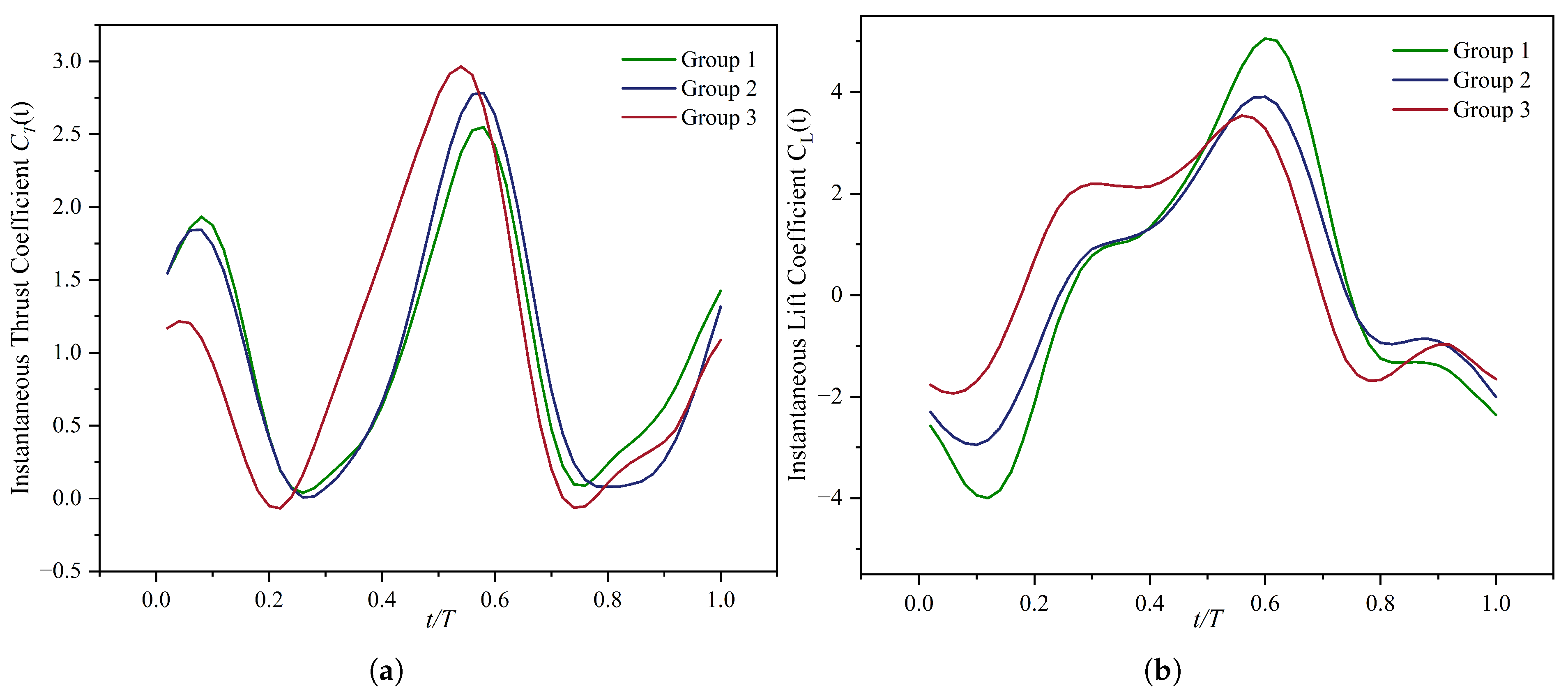
Figure 11 shows the evolution of the instantaneous thrust and lift coefficients over one period for the three parameter sets. In Figure 11a, none of the sets produces negative thrust within the cycle; moreover, Group 3 attains both the largest peak C T ( t ) and the highest mean thrust coefficient. In Figure 11b, the instantaneous lift coefficient C L ( t ) exhibits two extrema (one positive and one negative) per cycle; the extremal magnitudes decrease from Group 1 to Group 3, with Group 3 being the smallest. Overall, Group 3 yields the largest mean thrust and the smallest mean lift, indicating more effective conversion of input power into net propulsive thrust rather than into induced-drag-related lift, hence higher propulsive efficiency and lower power demand for a given thrust level.
Adjusting the relative thickness t * , relative camber f * , and the location of relative camber x f * primarily targets optimization of the flapping hydrofoil’s leading-edge geometry. Figure 12 shows surface-pressure contours at t = 0.4 T for the three parameter sets. Distinct pressure patterns emerge: the magnitude and extent of the high-pressure region near the leading edge increase progressively, while the low-pressure region contracts and shifts forward toward the leading edge. Consequently, the pressure difference between the upper and lower surfaces grows from Group 1 to Group 3, with the third configuration attaining the peak thrust.
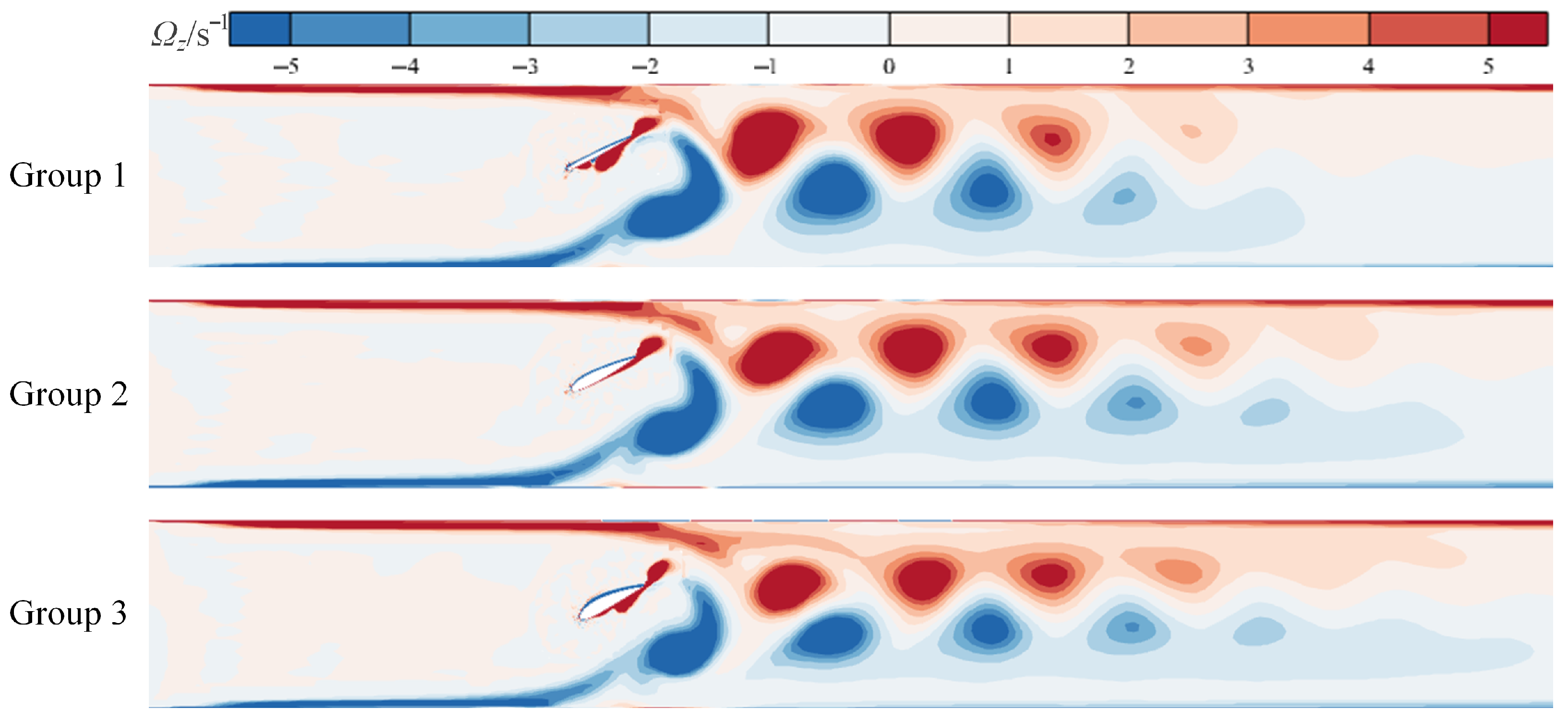
When the flapping hydrofoil follows its prescribed periodic kinematics, a jetting effect arises: in each cycle, a negative and a positive vortex are shed from the lower and upper surfaces, respectively. The counter-rotating vortex pair convects downstream and dissipates, forming in the wake an alternating street with positive vortices below and negative vortices above. This pattern is opposite to the classical von Kármán vortex street and is therefore termed a reverse von Kármán vortex street.
To further clarify why Group 3 achieves the best propulsive performance, Figure 13 shows vorticity contours at t = 0.4 T for the three parameter sets. The Group 1 hydrofoil exhibits a relatively loose, disordered vortex street, with large spacing between opposite-sign vortex cores and structures located close to the boundary. By contrast, Group 3 forms a more compact high-vorticity region tightly attached to the surface, with a strict spatial anti-phase arrangement that induces a stronger jet and reduces energy dissipation. Examination of the wake evolution further reveals a monotonic increase in vortex coherence from Groups 1 to 3, culminating in Group 3 with a clear, coherent chain-like vortex structure.

6. Conclusions

This paper proposes an MLP-DDQN method that, under small-sample conditions, rapidly identifies the Pareto-optimal set of flapping hydrofoil designs with respect to propulsive efficiency and averaged input power. An MLP-based surrogate of the simulation environment enables autonomous optimization by a DDQN augmented with Pareto-front information, thereby yielding recommended parameter combinations at prescribed power budgets. The paper further conducts a systematic assessment of how these combinations affect propulsion performance. The principal conclusions are as follows:
  • After training, the MLP-DDQN method rapidly locates multiple optima within the design domain using few samples and also returns competitive solutions near local optima. Relative to direct optimization in the original CFD environment, it achieves wall-time speedups of several orders of magnitude and requires only about 14.5 % of the samples used by conventional deep reinforcement learning, thereby improving training efficiency.
  • The Pareto set produced by the MLP-DDQN method exhibits a mean averaged input power of 106.58 W and a mean propulsive efficiency of 41.89 % . Moreover, with reward shaping, the optimal solutions obtained under different power constraints differ from the corresponding simulation targets by only 0.24 1.27 % .
  • Flow-field analyses across geometric parameter combinations indicate that a moderate rearward shift of the pitch-axis location, together with an appropriately shaped leading edge, promotes an orderly reverse von Kármán vortex street over the flapping hydrofoil, enhancing jet momentum transfer while reducing dissipation of shed vortices. This reduces energy loss and yields higher propulsive efficiency.
This study focuses exclusively on geometric-parameter optimization for the two-dimensional flapping hydrofoil and does not incorporate control of kinematic parameters. In addition, the generalization and robustness of the employed simulation environment remain to be validated. Future work will consider joint optimization over state and action parameters in a realistic channel flow to better support practical engineering applications.

Author Contributions

Conceptualization, J.Z.; methodology, X.Q.; software, X.Q.; validation, W.C., X.Q., and E.H.; formal analysis, E.H.; investigation, W.C.; resources, J.Z.; data curation, X.Q.; writing—original draft preparation, X.Q.; writing—review and editing, Y.S.; visualization, E.H.; supervision, X.Q.; project administration, J.Z.; funding acquisition, J.Z. All authors have read and agreed to the published version of the manuscript.

Funding

This research was funded by the Zhejiang Provincial Key Research and Development Project (Grant No. 2021C03019).

Data Availability Statement

Data are contained within the article.

Acknowledgments

The authors gratefully thank the Zhejiang Provincial Key Research and Development Project for their financial support.

Conflicts of Interest

The authors declare no conflicts of interest.

References

  1. Segura, E.; Morales, R.; Somolinos, J.A.; Lopez, A. Techno-Economic Challenges of Tidal Energy Conversion Systems: Current Status and Trends. Renew. Sustain. Energy Rev. 2017, 77, 536–550. [Google Scholar] [CrossRef]
  2. Picardi, G.; Astolfi, A.; Chatzievangelou, D.; Aguzzi, J.; Calisti, M. Underwater Legged Robotics: Review and Perspectives. Bioinspiration Biomim. 2023, 18, 031001. [Google Scholar] [CrossRef] [PubMed]
  3. Li, Z.; Chen, Y.; Zuo, X.; Jiang, Q.; Ye, X.; Xue, G. Hydrodynamic Performance Analysis and Diving Trajectory Prediction of a Novel Deep-Sea Lander with Flapping Hydrofoils. Ocean. Eng. 2024, 310, 118664. [Google Scholar] [CrossRef]
  4. Liu, Z.; Qu, H.; Song, X.; Chen, Z. A State-of-the-Art Review on Energy-Harvesting Performance of the Flapping Hydrofoil with Influential Parameters. Renew. Energy 2025, 245, 122849. [Google Scholar] [CrossRef]
  5. Xing, J.; Yang, L. Wave Devouring Propulsion: An Overview of Flapping Foil Propulsion Technology. Renew. Sustain. Energy Rev. 2023, 184, 113589. [Google Scholar] [CrossRef]
  6. Mohammed Arab, F.; Augier, B.; Deniset, F.; Casari, P.; Astolfi, J.A. Effects on Cavitation Inception of Leading and Trailing Edge Flaps on a High-Performance Hydrofoil. Appl. Ocean. Res. 2022, 126, 103285. [Google Scholar] [CrossRef]
  7. Zhao, W.; Liu, J.; Zhang, J.; Qin, J. Numerical Analysis of Effect of Bionic Hydrofoil Structure on Cavitation Suspension. J. Drain. Irrig. Mach. Eng. 2024, 42, 685–692, 700. [Google Scholar]
  8. Zhang, S.; Mei, L.; Zhou, J. Numerical Prediction of Hydrodynamic Performance of Differently Shaped Flapping Foil Propulsors. Chin. J. Ship Res. 2021, 16, 1. [Google Scholar] [CrossRef]
  9. Gupta, S.; Sharma, A.; Agrawal, A.; Thompson, M.C.; Hourigan, K. Role of Shape and Kinematics in the Hydrodynamics of a Fish-Like Oscillating Hydrofoil. J. Mar. Sci. Eng. 2023, 11, 1923. [Google Scholar] [CrossRef]
  10. Guo, C.; Zhang, Z.; Xu, P. Hydrodynamic Experiment and Mechanism of Improved Oscillating Hydrofoil. J. Huazhong Univ. Sci. Technol. (Natural Sci. Ed.) 2019, 47, 87–93. (In Chinese) [Google Scholar]
  11. Zhe, H.; Liu, Y.; Tan, J.; Si, X.; Yuan, P.; Wang, S. Influence of Different Vortex Generator Parameters on Hydrodynamic Characteristics of Tidal Current Turbine Hydrofoil. Acta Energiae Solaris Sin. 2022, 43, 350–356, (In Chinese with English Abstract). [Google Scholar] [CrossRef]
  12. Wang, L.; Xu, J.; Luo, W.; Luo, Z.; Xie, J.; Yuan, J.; Tan, A.C.C. A Deep Learning-Based Optimization Framework of Two-Dimensional Hydrofoils for Tidal Turbine Rotor Design. Energy 2022, 253, 124130. [Google Scholar] [CrossRef]
  13. Song, Z.; Zhu, J.; Lu, D. Optimization of Flapping Hydrofoil Propulsion Performance Based on Combined Neural Network and CFD. Acta Aerodyn. Sin. 2024, 42, 53–63. (In Chinese) [Google Scholar]
  14. Najafi, A.; Nowruzi, H.; Ghassemi, H. Performance Prediction of Hydrofoil-Supported Catamarans Using Experiment and ANNs. Appl. Ocean. Res. 2018, 75, 66–84. [Google Scholar] [CrossRef]
  15. Wang, L.; Xu, J.; Wang, Z.; Zhang, B.; Luo, Z.; Yuan, J.; Tan, A.C.C. A Novel Cost-Efficient Deep Learning Framework for Static Fluid–Structure Interaction Analysis of Hydrofoil in Tidal Turbine Morphing Blade. Renew. Energy 2023, 208, 367–384. [Google Scholar] [CrossRef]
  16. Yang, Y.; Wei, H.; Fan, D.; Li, A. Optimization Method of Underwater Flapping Foil Propulsion Performance Based on Gaussian Process Regression and Deep Reinforcement Learning. J. Shanghai Jiaotong Univ. 2025, 59, 70. [Google Scholar] [CrossRef]
  17. Kostas, K.V.; Ginnis, A.I.; Politis, C.G.; Kaklis, P.D. Shape-Optimization of 2D Hydrofoils Using an Isogeometric BEM Solver. Comput.-Aided Des. 2017, 82, 79–87. [Google Scholar] [CrossRef]
  18. Zhu, G.; Feng, J.; Li, P.; Wang, Z.; Wu, G.; Luo, X. Multi-Condition Optimisation Design of a Hydrofoil Based on Deep Belief Network. Ocean. Eng. 2023, 272, 113846. [Google Scholar] [CrossRef]
  19. Sun, Q.; Hua, E.; Sun, L.; Qiu, L.; Song, Y.; Xiang, M. Study on the Hydrodynamic Performance of Swing-Type Flapping Hydrofoil Bionic Pumps Affected by Foil Camber. Water 2024, 16, 595. [Google Scholar] [CrossRef]
  20. Hua, E.; Lu, C.; Xiang, M.; Song, Y.; Wang, T.; Sun, Q. Study on the Influence of Relative Chord Length and Frequency of Flapping Hydrofoil Device on Hydrodynamic Performance and Bank Slope Scour. Water 2025, 17, 1026. [Google Scholar] [CrossRef]
  21. Zhang, X.; Su, Y.; Yang, L.; Wang, Z. Hydrodynamic Performance of Flapping-Foil Propulsion in the Influence of Vortices. J. Mar. Sci. Appl. 2010, 9, 213–219. [Google Scholar] [CrossRef]
  22. Ji, B.; Luo, X.; Arndt, R.E.A.; Wu, Y. Numerical simulation of three-dimensional cavitation shedding dynamics with special emphasis on cavitation–vortex interaction. Ocean. Eng. 2014, 87, 64–77. [Google Scholar] [CrossRef]
  23. Shaheed, R.; Mohammadian, A.; Kheirkhah Gildeh, H. A comparison of standard kε and realizable kε turbulence models in curved and confluent channels. Environ. Fluid Mech. 2019, 19, 543–568. [Google Scholar] [CrossRef]
  24. Schouveiler, L.; Hover, F.S.; Triantafyllou, M.S. Performance of flapping foil propulsion. J. Fluids Struct. 2005, 20, 949–959. [Google Scholar] [CrossRef]
  25. West, D. Neural Network Credit Scoring Models. Comput. Oper. Res. 2000, 27, 1131–1152. [Google Scholar] [CrossRef]
  26. Mirjalili, S. How Effective Is the Grey Wolf Optimizer in Training Multi-Layer Perceptrons. Appl. Intell. 2015, 43, 150–161. [Google Scholar] [CrossRef]
  27. Tang, J.; Deng, C.; Huang, G.B. Extreme Learning Machine for Multilayer Perceptron. IEEE Trans. Neural Netw. Learn. Syst. 2016, 27, 809–821. [Google Scholar] [CrossRef] [PubMed]
  28. Talaei Khoei, T.; Ould Slimane, H.; Kaabouch, N. Deep Learning: Systematic Review, Models, Challenges, and Research Directions. Neural Comput. Appl. 2023, 35, 23103–23124. [Google Scholar] [CrossRef]
  29. Mnih, V.; Kavukcuoglu, K.; Silver, D.; Rusu, A.A.; Veness, J.; Bellemare, M.G.; Graves, A.; Riedmiller, M.; Fidjeland, A.K.; Ostrovski, G.; et al. Human-Level Control through Deep Reinforcement Learning. Nature 2015, 518, 529–533. [Google Scholar] [CrossRef]
  30. Arulkumaran, K.; Deisenroth, M.P.; Brundage, M.; Bharath, A.A. Deep Reinforcement Learning: A Brief Survey. IEEE Signal Process. Mag. 2017, 34, 26–38. [Google Scholar] [CrossRef]
  31. Hessel, M.; Modayil, J.; Van Hasselt, H.; Schaul, T.; Ostrovski, G.; Dabney, W.; Horgan, D.; Piot, B.; Azar, M.; Silver, D. Rainbow: Combining Improvements in Deep Reinforcement Learning. Proc. AAAI Conf. Artif. Intell. 2018, 32, 3215–3222. [Google Scholar] [CrossRef]
  32. Wang, Y.; Liu, H.; Zheng, W.; Xia, Y.; Li, Y.; Chen, P.; Guo, K.; Xie, H. Multi-Objective Workflow Scheduling with Deep-Q-Network-Based Multi-Agent Reinforcement Learning. IEEE Access 2019, 7, 39974–39982. [Google Scholar] [CrossRef]
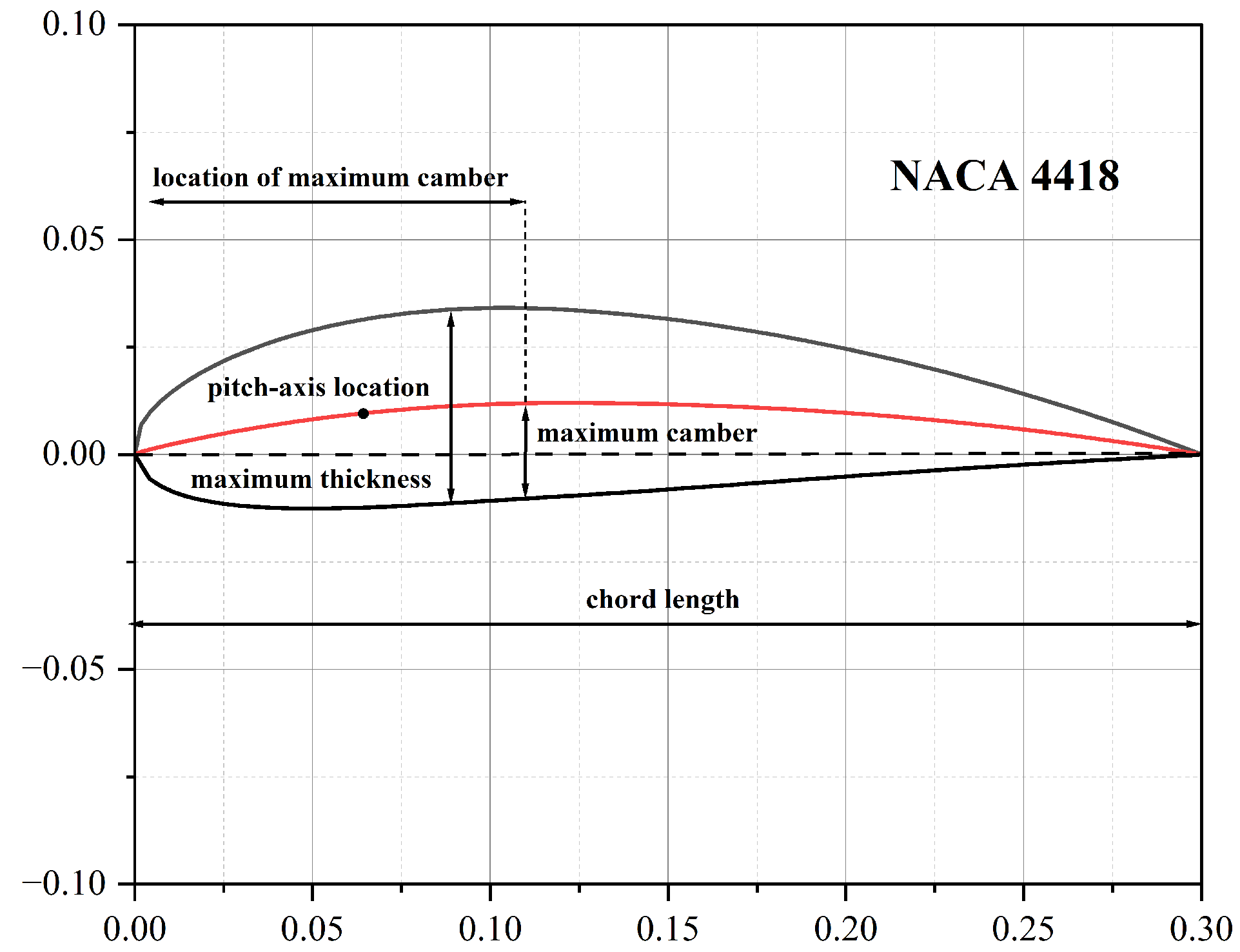
Figure 1. Profile of flapping hydrofoil and its main parameters.
Water 17 03290 g001
Figure 2. Schematic diagram of grid division of computational domain.
Water 17 03290 g002
Figure 3. Grid-independence verification.
Water 17 03290 g003
Figure 4. Comparison of numerical and experimental data.
Water 17 03290 g004
Figure 5. Schematic diagram of the MLP–DDQN workflow.
Water 17 03290 g005
Figure 6. Parity plots between true values (x-axis) and MLP predictions (y-axis): (a) propulsive efficiency; (b) averaged input power.
Water 17 03290 g006
Figure 7. Pareto frontier obtained by the DDQN during parameter optimization.
Water 17 03290 g007
Figure 8. DDQN training curves of the Q-network loss L Q and episode-averaged reward.
Water 17 03290 g008
Figure 9. Heatmap of parameter distributions and pairwise correlations for Pareto-optimal solutions.
Water 17 03290 g009
Figure 10. Normalized state trajectories for Pareto-front solutions during DDQN training.
Water 17 03290 g010
Figure 11. Time histories of C T ( t ) and C L ( t ) over one period T for the three parameter groups: (a) instantaneous thrust coefficient C T ( t ) ; (b) instantaneous lift coefficient C L ( t ) .
Water 17 03290 g011
Figure 12. Surface-pressure contours at t = 0.4 T for the three parameter sets.
Water 17 03290 g012
Figure 13. Vorticity contours at t = 0.4 T for the three parameter sets.
Water 17 03290 g013
Table 1. Parameters and value ranges.
ParameterValue Range
relative thickness t * {6, 9, 12, 15, 18, 24}
relative camber f * {0, 1, 2, 4}
location of relative camber x f * {0, 4}
pitch-axis location x p * [0, 50]
Table 2. Performance of the MLP surrogate on the training and validation sets.
TargetSetMAEMSE R 2 Training Time (s)Inference Time (ms)
averaged input powerTraining1.74858.08980.99615.90
Validation1.879410.84400.99440.27
propulsive efficiencyTraining0.0026 1.5 × 10 5 0.98677.73
Validation0.0028 2.0 × 10 5 0.98190.25
Table 3. Representative Pareto solutions and sample counts for MLP–DDQN vs. traditional CFD.
CategoryState VectorCFD [ P ( W ) , η ( % ) ] Prediction [ P ( W ) , η ( % ) ] MLP–DDQN SamplesTraditional CFD Samples
Algorithmic optimum[49.8, 18, 4, 4][104.52, 42.05][105.85, 41.67]6244300
averaged input power 120 W [42.5, 15, 4, 4][120.04, 41.47][118.77, 41.37]6244300
averaged input power 130 W [34.2, 15, 4, 2][129.94, 41.22][130.44, 41.64]6244300
averaged input power 140 W [29.2, 15, 4, 2][139.98, 40.86][139.13, 40.43]6244300
Table 4. Representative geometric parameter combinations and resulting performance.
ID x p * t * x f * f * Average Input Power (W)Propulsive Efficiency (%)
Group 120.0600189.6232.18
Group 230.01541140.3740.32
Group 349.81844104.5242.05
Disclaimer/Publisher’s Note: The statements, opinions and data contained in all publications are solely those of the individual author(s) and contributor(s) and not of MDPI and/or the editor(s). MDPI and/or the editor(s) disclaim responsibility for any injury to people or property resulting from any ideas, methods, instructions or products referred to in the content.