Article

Testing Machine Learning and Traditional Models for Tree-Ring-Based scPDSI Streamflow Reconstruction: A 1500-Year Record of the French Broad River, Tennessee, USA

by
Ray Lombardi
1,
Abel Andrés Ramírez Molina
2 and
Glenn Tootle
3,*
1
Department of Earth Sciences, University of Memphis, Memphis, TN 38152, USA
2
Department of Computer Science, University of Alabama, Tuscaloosa, AL 35487, USA
3
Department of Civil, Construction and Environmental Engineer, University of Alabama, Tuscaloosa, AL 35487, USA
*
Author to whom correspondence should be addressed.
Water 2025, 17(22), 3288; https://doi.org/10.3390/w17223288
Submission received: 9 October 2025 / Revised: 12 November 2025 / Accepted: 13 November 2025 / Published: 18 November 2025

Abstract

The French Broad River in eastern Tennessee is a critical water resource for the Tennessee Valley Authority’s hydropower and drought relief, yet its instrumental record spans less than a century. To evaluate new dendrochronological tools and examine long-term streamflow trends, we extended the stream record by 1500 years using linear regression and machine learning reconstruction models informed by the tree-ring-derived self-calibrating Palmer Drought Severity Index (scPDSI). Linear regression models provided skillful reconstruction and stable performance across calibration and validation periods. Random Forest and Deep Learning achieved higher skill but lost some of their skill advantage with validation periods, indicating overfitting. All models captured drought years more reliably than flood years, reflecting the sensitivity of scPDSI to soil moisture but its limitations for high-flow extremes in the Appalachian region. Trend analyses identified a significant change point in 1271 CE, separating a drought-dominated early period (500–1272 CE) from a wetter, less variable regime (1273–1970 CE). An emerging trend shows higher average flow interrupted by severe single-year droughts, consistent with regional evidence and projected changes to hydrologic regimes in Appalachia. These findings provide a millennial perspective on hydrologic extremes and guidance on using paleohydrology tools for water resource planning in a changing climate.

1. Introduction

Tree ring proxies of wet and dry conditions within watersheds provide critical insight into long-term streamflow variability [1]. Statistical relationships between tree ring measurements and streamflow have extended hydrologic records by centuries in many regions worldwide [2]. Over the past five decades, the growing number of tree ring chronologies archived in the International Tree-Ring Databank facilitated the development of gridded datasets that make these proxies broadly accessible for hydroclimate research [3]. Tree ring indices sensitive to precipitation and soil moisture inform gridded data assimilation of greater than 1000 years of precipitation and the self-calibrated Palmer Drought Severity Index (scPDSI) across the U.S. [4,5] and many other world regions [6]. Building on these advances, Ho and others [7] developed methods that leverage publicly available gridded scPDSI to reconstruct annual streamflow with high skill, transforming streamflow reconstructions into a widely accessible tool for the broader water resource community. As dendrochronological toolsets expand and incorporate new approaches from hydrology, including machine learning, it is increasingly important to evaluate the strengths and limitations of these integrative methods for understanding physical hydrological processes and informing water resource decision-making frameworks. Machine learning (ML) techniques, such as Random Forest and Deep Learning, provide flexible, non-linear frameworks for predicting streamflow [8,9,10]. While these algorithms often outperform traditional linear regression models by optimizing fits and achieving higher correlations between proxies and training datasets [11], they are also prone to overfitting when signal-to-noise ratios are low [8]. Jevšenak and others [12] recommend testing multiple ML approaches to determine the model best fitting the need for a particular study.
In this study, we reconstruct annual streamflow of the French Broad River using tree-ring-based scPDSI for the period 490–2005 CE. Previous work applying stepwise linear regression to tree ring-based streamflow records in other Tennessee River Basin headwaters produced skillful reconstructions [13], suggesting this approach provides a useful baseline for comparison. We take advantage of the long, unregulated gauged record at Newport, Tennessee, to perform a sensitivity analysis with a validation dataset, allowing us to evaluate the relative strengths and weaknesses of machine learning and traditional linear regression approaches in predicting streamflow and hydrologic extremes. Specifically, we aim to achieve the following: (1) determine whether machine learning techniques reliably improve predictive skill relative to linear regression; (2) assess how well tree ring proxies of scPDSI capture streamflow minima and maxima; and (3) evaluate long-term streamflow trends in the French Broad River over the last 1500 years. Our findings provide guidance for the application of machine learning algorithms in paleohydrology and for interpreting tree-ring-based scPDSI streamflow reconstructions.

2. Materials and Methods

2.1. Study Area

The French Broad River Basin drains an area of 4212 km2. The main stem originates in western North Carolina and flows into eastern Tennessee through the Blue Ridge Mountains, supplying much of the inflow to Douglas Lake Reservoir (Figure 1). Surficial geology consists of ~2–5 m thick saprolites developed on Proterozoic gneiss and granite, as well as bouldery to clayey residuum with highly variable depths of 2–30 m formed on Paleozoic sedimentary rocks [14]. Groundwater is limited by residuum depths and fracture networks within metamorphic and igneous rocks, making surface water the critical water resource in this region.
This study used the U.S. Geological Survey (USGS) stream gauge on the French Broad River near Newport, Tennessee, (#03455000), which records monthly, unregulated streamflow from 1921 to 2022. Streamflow during this period shows clear seasonality, with higher flows in winter and spring and lower flows in late summer and fall (Figure 1). Precipitation in the French Broad region is generated by four primary storm types: (1) mid-latitude cyclones, often associated with slow-moving frontal systems during the cool season; (2) meso-scale frontal systems; (3) localized convective storms during the warm season; and (4) occasional tropical remnant storms from June through October [15]. Among these, slow-moving mid-latitude cyclones are the most frequent precipitation source [15]. Historically, winter and spring received the largest precipitation totals [16]. However, since the 1980s, precipitation seasonality has shifted: summer and fall totals have increased while cool-season precipitation has declined, consistent with intensification and a westward expansion of the North Atlantic Subtropical High [16,17].

2.2. Streamflow Reconstruction

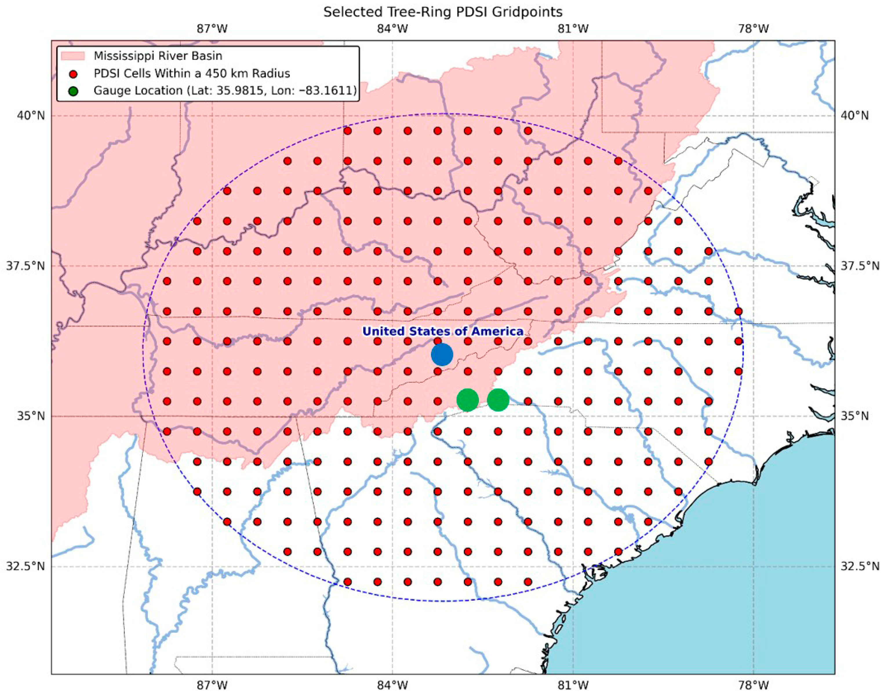
We applied four statistical and machine learning approaches to reconstruct annual streamflow using gridded self-calibrated Palmer Drought Severity Index (scPDSI) data from the North American Drought Atlas [18], extracted within a 450 km radius of the French Broad River gauge (Figure 2) [7]. The scPDSI series provide proxies for soil moisture and are recognized as reliable predictors of streamflow [7]. For the target dataset, we calculated total annual streamflow volume (millions of cubic meters, MCM) from continuous monthly discharge records at the French Broad River gauge spanning 1921–1994 (74 years). Reconstructions were developed using two calibration periods: the full 74-year record (1921–1994) and a 50-year subset (1940–1989 to match the period used in the Deep Learning, Random Forest, and Generalized Learning models).
Our first approach employed stepwise linear regression (SLR), a common and robust method in dendrohydrology that iteratively identifies the most skillful scPDSI predictors of streamflow. Prior to developing the SLR models, two pre-screening steps were implemented. First, each scPDSI vector within the 450 km search radius (Figure 2) was correlated with the streamflow vector for the overlapping period of record. Positively correlated scPDSI vectors (cells) that achieved 99% (p < 0.01) significance were identified. This subset of scPDSI cells was examined for stabilization such that a “moving correlation window” was applied to the retained scPDSI cells (99% positively significant) and the streamflow vector. The moving correlation window was approximately one-third of the entire record, and scPDSI cells were retained if no negative correlations were observed. Stabilization was performed to verify whether, while overall correlation for the entire period of record was 99% positively significant, there were periods within the entire period record observed in which scPDSI and streamflow were poorly correlated (i.e., negative correlation). The scPDSI cells which passed these two pre-screening steps were next utilized as predictors (independent variables) in the SLR models. The skills from the SLR results (Table 1) establish a strong baseline measure of predictive skill from scPDSI in the basin. Only one cell remained for each calibration period, making each model a simple regression rather than a multi-regression. The pre-screening procedure, however, selected different scPDSI cells that best predicted the 74-year calibration record and the 50-year calibration record, which is why two cells are highlighted in Figure 2. In addition, we implemented three machine learning methods: (1) Deep Learning (DL: a two-layer artificial neural network), (2) Random Forest (RF: an ensemble regression based on decision tree algorithm), and (3) a Generalized Linear Model (GLM: utilizes an adaptive selection of distribution family and link functions). Each of the four approaches were applied to both calibration periods, producing eight reconstructions in total. We applied a bias correction procedure with a quantile mapping approach which systematically adjusts predicted and observed values in all reconstructions [19]. A final ensemble reconstruction was generated by averaging predictions across six models. Reconstructions from DL and RF trained on data from the full observed period (74-years) were excluded due to overfitting.
All modeling and statistical analyses were conducted using a combination of open-source and licensed software environments. The SLR models were developed using the PALEO-RECON software v 1.0 tool introduced by [20], a Python-based platform for automated reconstruction modeling that streamlines tree ring proxy integration and regression workflows. Machine learning models (RF, GLM, and DL) were implemented in Altair AI Studio 2024.0.0. (formerly RapidMiner) with k-fold cross-validation and hyperparameter optimization to identify the most robust configurations. Trend and change-point analyses (Pettitt, Mann–Kendall, and Sen’s Slope) were conducted in R version 4.3.1 using the trend package [21].

2.3. Sensitivity Analyses

We evaluated reconstruction skill of model estimates by calculating the squared correlation (r2) between observed flows and each of the reconstructions derived from different models and calibration datasets. For the SLR models, model skill was evaluated by R2 predicted (applying drop-one cross validation), Variance Inflation Factor (VIF), and Durbin–Watson (model overfitting and model multi-collinearity). For each year (sign test) in the overlapping period of record, the modeled value is subtracted from the observed value, and the number of positive and negative outcomes were counted. The statistical significance (p-value) was determined next using the Minitab software v 21.1.0 which applied a one-sample sign test to this data. To test how well reconstructions captured extremes, we classified years below the 20th percentile of observed flows as low-flow years and those above the 80th percentile as high-flow years. To evaluate differences in model performance in predicting minima and maxima, we calculated R2 of flow in low- and high-flow years between modeled and observed flows within these subsets. We then compared performance between low- and high-flow years using paired t-tests on model-specific R2 values.

2.4. Trend Analysis

Moving averages spanning 5, 10, and 20 years were applied to the total annual flow reconstruction to reduce noise and enhance trend detection. Pettitt tests for non-parametric trend detection of all filtered time series were performed using the trend package in R [21,22]. The Pettitt test more reliably detects departures from the central tendency in streamflow populations with fewer spurious points than parametric change-point tests [23,24,25]. Finally, Mann–Kendall and Sen’s Slope tests were performed to test the significance, strength, and directionality of trends in streamflow in the full and partial time series (before and after the change point).

3. Results

3.1. Modeled Streamflow Reconstruction

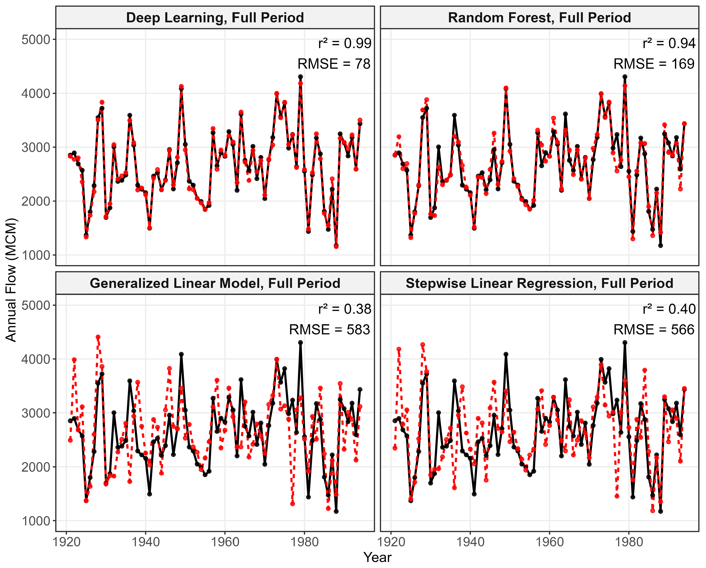
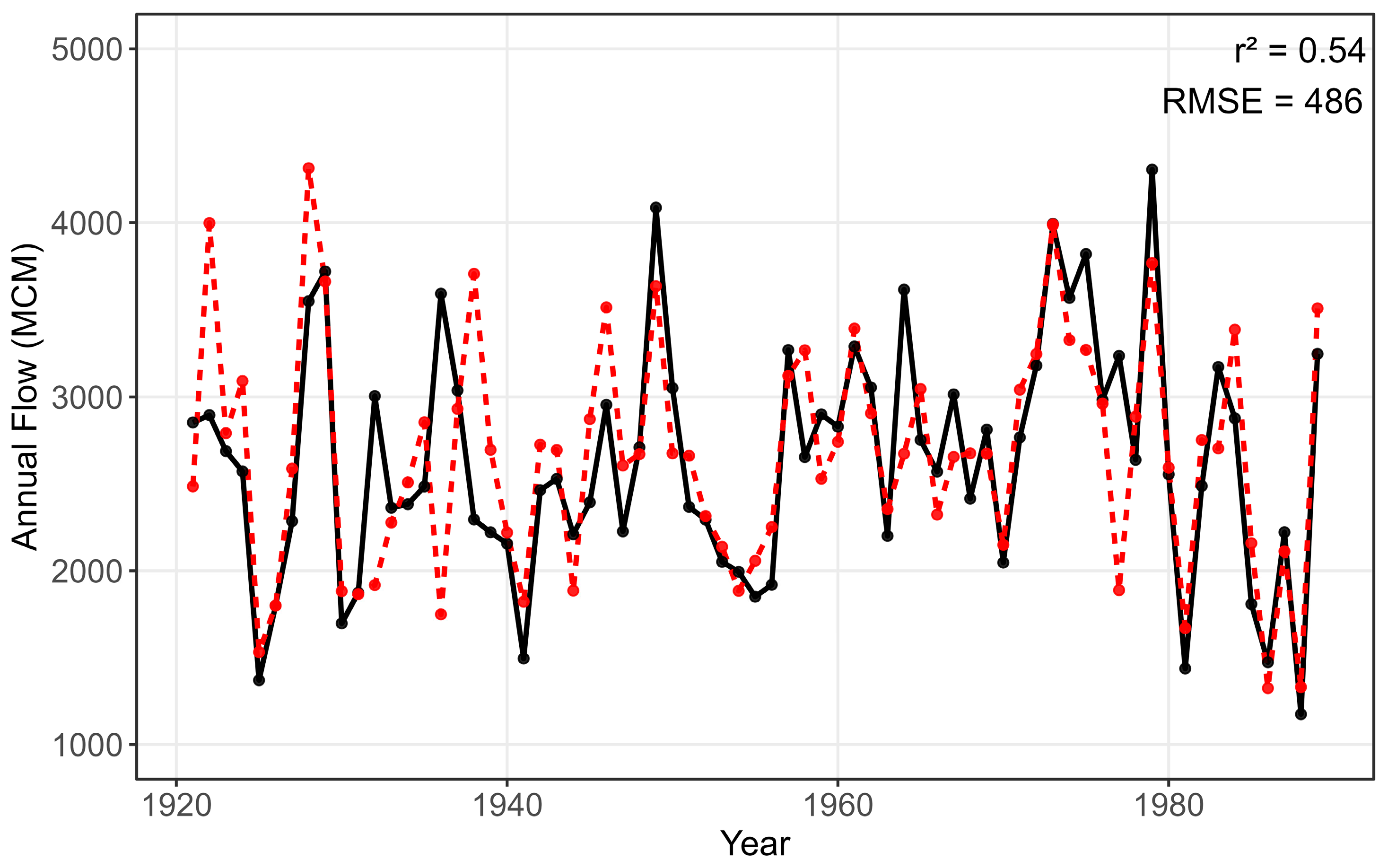
The machine learning models, Deep Learning and Random Forest, had higher calibration accuracy than the linear models, Generalized Linear Model and Stepwise-Linear Regression, in every calibration period (Figure 3 and Figure 4). The shorter calibration periods of 50 years showed that accurate scPDSI prediction of streamflow decreased in years outside of the training datasets. Validation data provided by flow observations prior to the 50 years of the highest correlated scPDSI from 1940 to 1989 revealed that the skill of all models decreases outside of the calibration period, and the machine learning approach lost all advantages to linear regression models in predicting streamflow (Table 2). The model performed well (r2 = 0.54, Figure 5), while reconstruction skill remained more stable than using machine learning techniques only.
Reconstruction skill differed significantly between low- and high-flow years. The four full period models contained 16 high flow and 15 low flows, while all other models contained 14 high and low flow years. The correlation values were consistently higher in low-flow years than in high-flow years (Table 3). Averaged across models, 50-yr reconstructions explained 60% of minima but only 20% of maxima variance, with consistent overprediction of low flows (+100 MCM) and underprediction of high flows (−300 MCM). The model calibrated for the full period improved balance, explaining 75% of drought variance and 45% of flood variance, though bias patterns persisted. A paired t-test indicated with high significance (p = 0.0005) that scPDSI-based streamflow reconstructions predicted streamflow minima more accurately than maxima, with r2 averaging 0.37 higher in low-flow years.

3.2. Temporal Characteristics of Streamflow

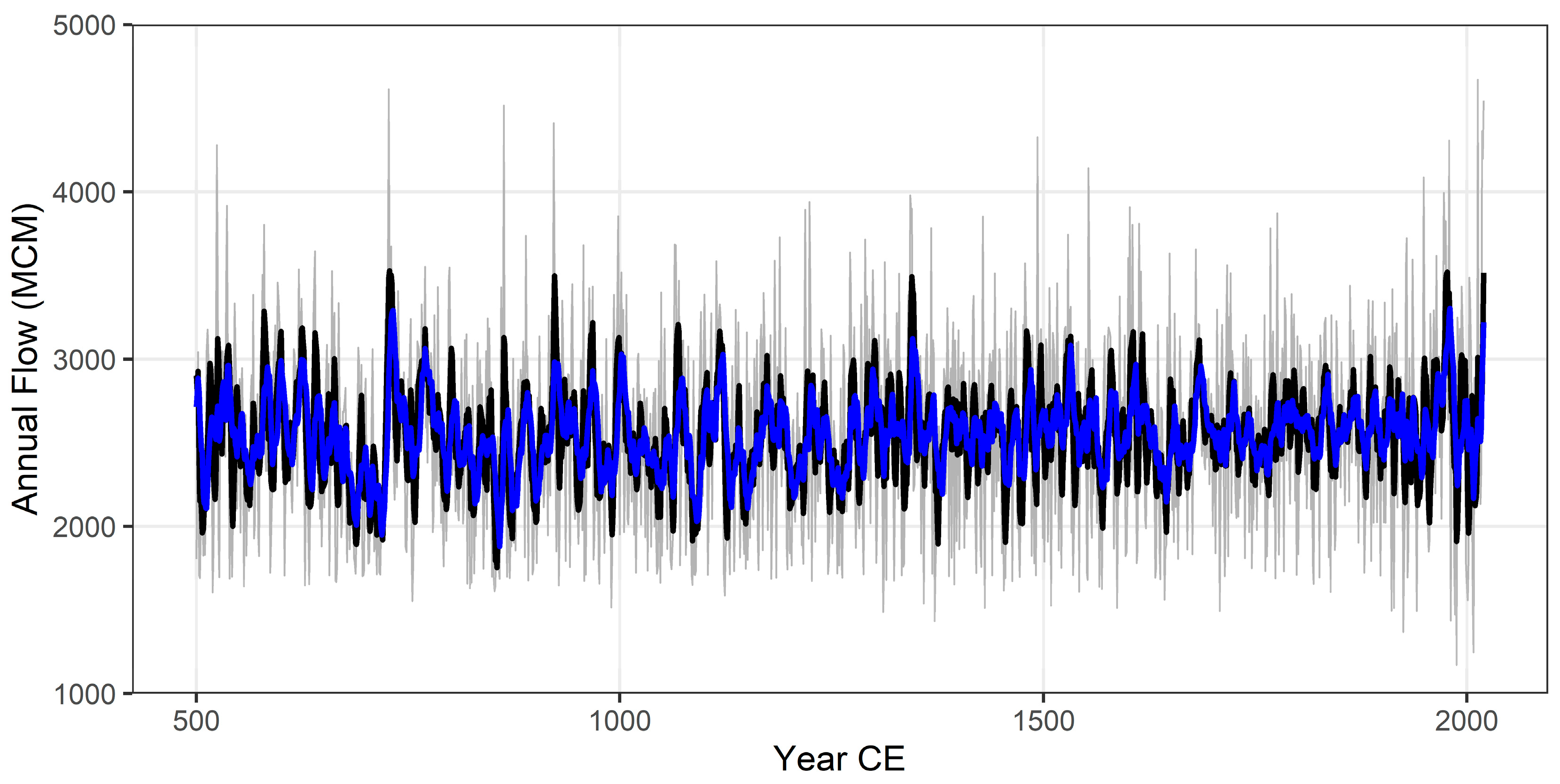
Filtered streamflow time series from the model ensemble, including a 5-year and 10-year moving average, made trends and variation more apparent than unfiltered data. Both filtered time series captured the timing of abrupt increases with subtle differences in magnitude, for example, ~730 CE (Figure 6). Unless otherwise stated, trend analyses utilized the 5-year filter of streamflow because the 10-year filter does not provide additional insights.
Pettitt’s test identified a highly significant (p < 0.001) change point at 1272 CE in the 5-year filtered flow series (Figure 7). The unfiltered and 10-year filtered flow series also produced significant change points in 1272, suggesting a robust detection. Mean streamflow increased slightly, and sample variance decreased by 30% after the 1272 CE change point. Despite only subtle changes in each period’s mean values, a Mann–Kendall test for the full period suggests a significant (p = 0.001) monotonic trend toward the present. A Sen’s Slope (S) test over the full reconstruction shows a modest (S = 0.082) but highly significant (p < 0.001) increasing trend in flow. There were more nuanced trends between significant periods. A significant negative streamflow trend (S = −0.11; p = 0.03) occurred between 500 and 1271 CE. After the changepoint, streamflow did not significantly trend (p = 0.3). The authors acknowledge that the earliest period of the streamflow reconstruction will likely be the most uncertain given the reduced number of tree ring chronologies used to generate the scPDSI proxies.

4. Discussion

4.1. Sensitivity Analyses of Reconstruction Approaches

The long, unregulated gauged record of the French Broad River at Newport, Tennessee, allowed us to validate predictive models and assess the strengths and weaknesses of four reconstruction approaches. Deep Learning and Random Forest provided near-perfect accuracy within their training periods but lost much of their advantages in validation. In contrast, the Generalized Linear Model and Stepwise Linear Regression performed with lower overall skill yet maintained stability across calibration and validation, suggesting that linear models are robust and better suited for temporal extension. These findings align with Woodhouse [8], who cautioned that artificial neural networks tend to overfit training data compared with linear models. Our results also show similar overfitting in the decision-tree structure of Random Forest. By averaging across all approaches, the model ensemble balanced the high skill of machine learning methods with the robustness of linear regression models, achieving strong skill for the full observed period (R2 = 0.54) and only moderate skill loss in validation.
Machine learning approaches in hydrology benefit from diverse training datasets to improve identification of similarities and dissimilarities [26]. Although our approach adapted from Ho et al. [7] uses a wide search diameter (450 km) to identifying well-correlated scPDSI reconstructions, it is possible that this approach does not provide heterogenous datasets necessary to allow flexible prediction in ML approaches. Additionally, most localities have only short records for training predictive models which combined with a lack of constraints in ML approaches may exacerbate extrapolation errors and failure to predict emerging patterns [27]. Reconstructions for streams on the regional scale (i.e., multiple basins) rather than at-site gauge reconstruction may provide ML approaches with data-rich environments that optimize their non-linear functions.
Tree ring streamflow reconstructions are used to contextualize long-term hydrologic regimes [1], often with a focus in extreme drought [28]. In this study, we found that all reconstruction models are significantly more skilled in predicting low flows than high flows, suggesting tree-ring-based streamflow reconstructions provide the best insight into the magnitude of hydrologic drought. High-flow years were underestimated in 60% of all occurrences and by an average of 282 MCM across all models. For the year 1936, six of nine models underestimated flow severely enough that reconstructions predicted a less than 20th percentile flow occurred, when an 80th percentile flow actually occurred. Streamflow in the French Broad River is highly variable across annual and centennial timescales, and sediment-based paleoflood reconstructions revealed floods occurred often during droughts [29]. Floods are driven by extreme precipitation and excess soil moisture. In the eastern U.S., PDSI is not a strong indicator of extreme precipitation [30] and is therefore more likely to underpredict flood flows generated by extreme precipitation in years where soil moisture does not recover. Interestingly, high flow years were overpredicted in 41% of cases, which may be explained by attenuation of runoff and flows in wet PDSI years.
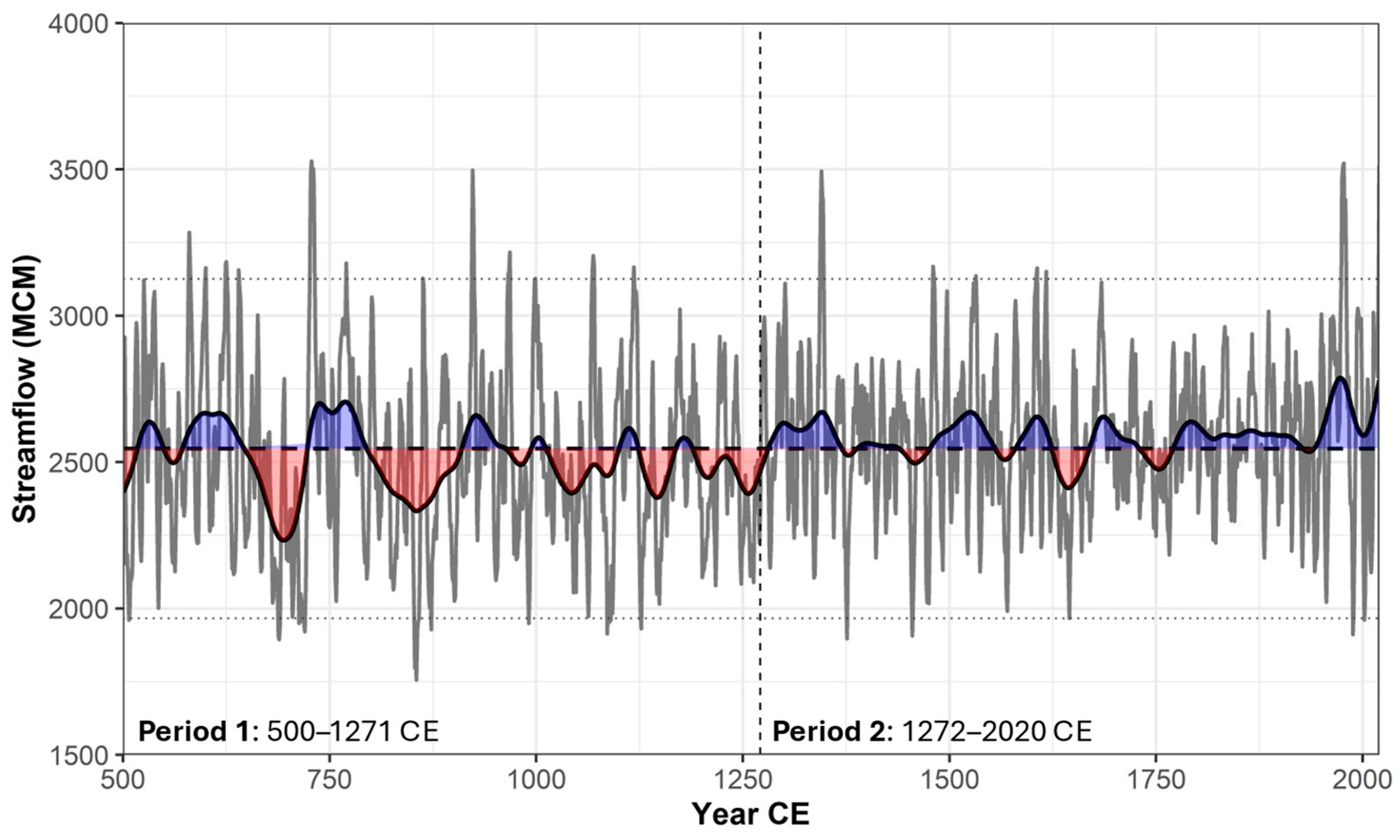
Together, these results highlight that scPDSI-based streamflow reconstructions are useful for characterizing hydrologic drought but lack sensitivity to flood variability in the French Broad River. While the use of scPDSI likely contributed to reduced skill in predicting high flows, Sahour et al. [31] also reported low R2 values when directly relating tree growth to high streamflow, suggesting that trees may be less sensitive to the upper end of streamflow distributions. Capturing the full spectrum of hydrologic extremes, therefore, requires a multiproxy framework, combining tree ring reconstructions of drought with proxies sensitive to peak discharge, such as overbank flood sediments or flood-stage paleoflood records [29].

4.2. Long-Term Flow Trends

The average annual streamflow of the French Broad River has increased gradually but significantly over the past 1500 years. A major change point in 1271 CE divided the record into two distinct periods. The first period (500–1271 CE) showed a strong decreasing trend in streamflow and prolonged, more intense droughts, as indicated by 30-year cubic splines representing climate norms (Figure 7). The second period (1272–2020 CE) was marked by reduced variability and generally wetter climate norms (Figure 7). The contrast between a strong decline before 1271 and the absence of any trend afterward suggests that the long-term rise across the full record stems from the reduced severity and frequency of droughts in recent centuries. This pattern points to hydrologic recovery following the Medieval Warm Period (900–1300 CE) and illustrates how persistent climate regimes can obscure or exaggerate long-term trends.
Megadroughts, representing widespread and intense drought, have occurred across North America several times over the past 2000 years. Long-term streamflow reconstructions (i.e., 30-year splines) indicate thirteen dry periods with below-mean flow in the French Broad River basin since 500 CE (Figure 7). The most persistent dry period from 796 to 910 CE in the French Broad River basin temporally coincides with a prominent multi-century North American megadrought [32] associated with persistent La Niña conditions [33]. A review of North American megadroughts during the Common Era does not include paleo-records from the southeastern United States; nevertheless, our study corroborates several megadroughts between 800 and 1300 CE and during the late 16th century (this study’s drought: 1550–1578 CE) [32]. More broadly, the long-term trend toward drier conditions before approximately 1250 CE followed by generally wetter centuries thereafter is remarkably consistent with the synthesis of hydroclimate proxies by Rodysill et al. [34], suggesting a robust change point detection.
The long-term mean flow indicates that the French Broad River has become wetter since 1970. This trend is consistent with other long-term streamflow trends observed in the Eastern United States [13,35,36,37,38]. Yet, streamflow records since 1970 also contained one of our 1500-year record’s most severe single-year droughts that occurred in 1988 (Table 4). Increased inter-annual hydrologic variability since 1970 represents a departure from earlier centuries of Period 2 and may signal an emerging trend that is not yet statistically detectable in our longer record. Several regional streamflow studies support an abrupt increase in streamflow since 1970 [38,39,40] in response to increased precipitation [41]. However, this step change reflects a departure from the mean rather than a continuous rise [38]. Future mean streamflow will likely remain higher over the next century in the Appalachian region of the United States [42,43], but single-year severe hydrological drought will also likely continue at a higher frequency than the 20th century as rising temperatures drive greater evaporative demand [44].

5. Conclusions

This study presents the first 1500-year annual streamflow reconstruction for the French Broad River, developed from tree-ring-based scPDSI using both linear regression and machine learning techniques. By leveraging the long, unregulated gauged record at Newport, Tennessee, we evaluated reconstruction skill across approaches, calibration windows, and hydrologic extremes.
Our results show that machine learning models (RF, DL) achieve high predictive accuracy within calibration periods but lose skill in validation, indicating overfitting, while linear models (GLM, SLR) maintain greater robustness over time. An ensemble approach, averaging across all models, provided the best balance between skill and stability, with an overall R2 of 0.6. Across all models, reconstructions captured low-flow years more reliably than high-flow years, underscoring the strength of tree ring proxies for characterizing hydrologic drought but also their limitations in representing high-flow extremes.
Together, these results highlight both the opportunities and limitations of integrating machine learning methods for applying dendrohydrology tools like tree-ring-based scPDSI. PDSI-based streamflow reconstructions provide critical paleo perspectives on hydrologic variability, but capturing the full spectrum of hydrologic extremes requires multiproxy frameworks that combine tree ring reconstructions with sediment-based paleoflood records. In the context of ongoing and projected climate change, our findings suggest that the Appalachian region is likely to experience higher mean flows alongside more frequent drought extremes, posing compounding challenges for water resource management.

Supplementary Materials

The following supporting information can be downloaded at: https://www.mdpi.com/article/10.3390/w17223288/s1, Table S1: French Broad River Dataset.

Author Contributions

Conceptualization, R.L. and G.T.; methodology, R.L., A.A.R.M. and G.T.; software, R.L. and A.A.R.M.; validation, R.L. and G.T.; formal analysis, R.L. and G.T.; investigation, R.L.; resources, G.T.; data curation, G.T.; writing—original draft preparation, R.L. and G.T.; writing—review and editing, R.L., A.A.R.M. and G.T.; visualization, R.L.; project administration, G.T.; funding acquisition, G.T. All authors have read and agreed to the published version of the manuscript.

Funding

This study was supported by the National Science Foundation under Award No. 2152140.

Data Availability Statement

The original contributions presented in this study are included in the article/Supplementary Material. Further inquiries can be directed to the corresponding author.

Acknowledgments

The authors wish to thank The University of Alabama, Alabama Water Institute (AWI), and the Cooperative Institute for Research to Operations in Hydrology (CIROH) for their institutional support. Additionally, the authors thank two reviewers for their constructive feedback and insightful comments.

Conflicts of Interest

The authors declare no conflicts of interest.

Abbreviations

The following abbreviations are used in this manuscript:
CECommon Era
DLDeep Learning
GLMGeneralized Linear Model
km2Square kilometers
m3Cubic meters
MCMMillion cubic meters
MLMachine Learning
PDSIPalmer Drought Severity Index
RR statistical computing environment/language
R2Model decimal proportion of variance explained
r2Squared Pearson’s correlation
RFRandom Forest
RMSERoot-mean-square error
scPDSISelf-calibrating Palmer Drought Severity Index
SLRStepwise Linear Regression
TVATennessee Valley Authority
U.S.United States
USGSUnited States Geological Survey
VIFVariance Inflation Factor
yrYear

References

  1. Meko, D.M.; Woodhouse, C.A. Application of streamflow reconstruction to water resources management. In Dendroclimatology: Progress and Prospects; Hughes, M.K., Swetnam, T.W., Diaz, H.F., Eds.; Springer: Dordrecht, The Netherlands, 2010; pp. 231–261. [Google Scholar]
  2. Meko, D.M.; Woodhouse, C.A.; Morino, K. Dendrochronology and links to streamflow. J. Hydrol. 2012, 412, 200–209. [Google Scholar] [CrossRef]
  3. Guiterman, C.H.; Gille, E.; Shepherd, E.; McNeill, S.; Payne, C.R.; Morrill, C. The International Tree-Ring Data Bank at fifty: Status of stewardship for future scientific discovery. Tree-Ring Res. 2024, 80, 13–18. [Google Scholar] [CrossRef]
  4. Stahle, D.W.; Cook, E.R.; Burnette, D.J.; Torbenson, M.C.; Howard, I.M.; Griffin, D.; Diaz, J.V.; Cook, B.I.; Williams, A.P.; Watson, E.; et al. Dynamics, variability, and change in seasonal precipitation reconstructions for North America. J. Clim. 2020, 33, 3173–3195. [Google Scholar] [CrossRef]
  5. Cook, E.R.; Seager, R.; Heim, R.R., Jr.; Vose, R.S.; Herweijer, C.; Woodhouse, C. Megadroughts in North America: Placing IPCC projections of hydroclimatic change in a long-term palaeoclimate context. J. Quat. Sci. 2010, 25, 48–61. [Google Scholar] [CrossRef]
  6. Cook, E.R.; Seager, R.; Kushnir, Y.; Briffa, K.R.; Büntgen, U.; Frank, D.; Krusic, P.J.; Tegel, W.; van der Schrier, G.; Andreu-Hayles, L.; et al. Old World megadroughts and pluvials during the Common Era. Sci. Adv. 2015, 1, e1500561. [Google Scholar] [CrossRef]
  7. Ho, M.; Lall, U.; Cook, E.R. Can a paleodrought record be used to reconstruct streamflow? A case study for the Missouri River Basin. Water Resour. Res. 2016, 52, 5195–5212. [Google Scholar] [CrossRef]
  8. Woodhouse, C.A. Artificial neural networks and dendroclimatic reconstructions: An example from the Front Range, Colorado, USA. Holocene 1999, 9, 521–529. [Google Scholar] [CrossRef]
  9. Gangopadhyay, S.; Harding, B.L.; Rajagopalan, B.; Lukas, J.J.; Fulp, T.J. A nonparametric approach for paleohydrologic reconstruction of annual streamflow ensembles. Water Resour. Res. 2009, 45, 1653–1659. [Google Scholar] [CrossRef]
  10. Li, J.; Wang, Z.; Lai, C.; Zhang, Z. Tree-ring-width based streamflow reconstruction based on the random forest algorithm for the source region of the Yangtze River, China. Catena 2019, 183, 104216. [Google Scholar] [CrossRef]
  11. Jevšenak, J.; Levanič, T. Should artificial neural networks replace linear models in tree-ring based climate reconstructions? Dendrochronologia 2016, 40, 102–109. [Google Scholar] [CrossRef]
  12. Jevšenak, J.; Levanič, T.; Džeroski, S. Comparison of an optimal regression method for climate reconstruction with the compare_methods() function from the dendroTools R package. Dendrochronologia 2018, 52, 96–104. [Google Scholar] [CrossRef]
  13. Anderson, S.; Ogle, R.; Tootle, G.; Oubeidillah, A. Tree-ring reconstructions of streamflow for the Tennessee Valley. Hydrology 2019, 6, 34. [Google Scholar] [CrossRef]
  14. Colquhoun, D.J.; Friddell, M.S.; Wheeler, W.H.; Daniels, R.B.; Gregory, J.P.; Miller, R.A.; Van Nostrand, A.K. Quaternary Geologic Map of the Savannah 4° × 6° Quadrangle, United States; U.S. Geological Survey Miscellaneous Investigations Series Map I–1420 (NI–17); U.S. Geological Survey: Reston, VA, USA, 1987; scale 1:1,000,000.
  15. Schaefer, M.; Barker, B.; Carney, S.; Gibson, W.; Martin, D.; Parzybok, T.; Taylor, G. Regional Precipitation-Frequency Analyses for Mid-Latitude Cyclones, Mesoscale Storms with Embedded Convection, Local Storms and Tropical Storm Remnant Storm Types in the Tennessee Valley Watershed; Report to Tennessee Valley Authority, 2015. Available online: https://mgsengr.com/wp-content/download/TVA_Point%20Precipitation-Frequency_2015-03-02_Release.pdf (accessed on 5 October 2025).
  16. Jones, J.R.; Schwartz, J.S.; Ellis, K.N.; Hathaway, J.M.; Jawdy, C.M. Temporal variability of precipitation in the Upper Tennessee Valley. J. Hydrol. Reg. Stud. 2015, 3, 125–138. [Google Scholar] [CrossRef]
  17. Li, W.; Li, L.; Fu, R.; Deng, Y.; Wang, H. Changes to the North Atlantic subtropical high and its role in the intensification of summer rainfall variability in the southeastern United States. J. Clim. 2011, 24, 1499–1506. [Google Scholar] [CrossRef]
  18. Cook, E.R.; Lall, U.; Woodhouse, C.A.; Meko, D.M. NOAA/WDS Paleoclimatology—Cook et al. 2004 North American Drought Atlas PDSI Reconstructions; NOAA National Centers for Environmental Information: Boulder, CO, USA, 2005. [CrossRef]
  19. Robeson, S.M.; Maxwell, J.T.; Ficklin, D.L. Bias correction of paleoclimatic reconstructions: A new look at 1200+ years of Upper Colorado River flow. Geophys. Res. Lett. 2020, 47, e2019GL086689. [Google Scholar] [CrossRef]
  20. Ramírez Molina, A.A.; Tootle, G.; Formetta, G.; Piechota, T.; Gong, J. Extraordinary 21st Century Drought in the Po River Basin (Italy). Hydrology 2024, 11, 219. [Google Scholar] [CrossRef]
  21. Pohlert, T. trend: Non-Parametric Trend Tests and Change-Point Detection; R Package v1.4; 2023; Available online: https://brieger.esalq.usp.br/CRAN/web/packages/trend/vignettes/trend.pdf (accessed on 5 October 2025). [CrossRef]
  22. R Core Team. R: A Language and Environment for Statistical Computing; R Foundation for Statistical Computing: Vienna, Austria, 2024; Available online: https://www.R-project.org/ (accessed on 5 October 2025).
  23. Mallakpour, I.; Villarini, G. A simulation study to examine the sensitivity of the Pettitt test to detect abrupt changes in mean. Hydrol. Sci. J. 2016, 61, 245–254. [Google Scholar] [CrossRef]
  24. Ryberg, K.R.; Hodgkins, G.A.; Dudley, R.W. Change points in annual peak streamflows: Method comparisons and historical change points in the United States. J. Hydrol. 2020, 583, 124307. [Google Scholar] [CrossRef]
  25. Hodgkins, G.A.; Over, T.M.; Dudley, R.W.; Russell, A.M.; LaFontaine, J.H. The consequences of neglecting reservoir storage in national-scale hydrologic models: An appraisal of key streamflow statistics. JAWRA J. Am. Water Resour. Assoc. 2024, 60, 110–131. [Google Scholar] [CrossRef]
  26. Fang, K.; Kifer, D.; Lawson, K.; Feng, D.; Shen, C. The data synergy effects of time-series deep learning models in hydrology. Water Resour. Res. 2022, 58, e2021WR029583. [Google Scholar] [CrossRef]
  27. Xu, T.; Liang, F. Machine learning for hydrologic sciences: An introductory overview. Wiley Interdiscip. Rev. Water 2021, 8, e1533. [Google Scholar] [CrossRef]
  28. Martin, J.T.; Pederson, G.T.; Woodhouse, C.A.; Cook, E.R.; McCabe, G.J.; Wise, E.K.; Erger, P.; Dolan, L.; McGuire, M.; Gangopadhyay, S.; et al. 1200 years of Upper Missouri River streamflow reconstructed from tree rings. Quat. Sci. Rev. 2019, 224, 105971. [Google Scholar] [CrossRef]
  29. Davis, M.L.; Lombardi, R.; Gage, M.D.; Tootle, G.; Rittenour, T.; Quimby, A.C. High and dry: A ~300-year record of hydrologic extremes from the French Broad River in the southeastern US. J. Hydrol. Reg. Stud. 2025, 61, 102673. [Google Scholar] [CrossRef]
  30. Steinschneider, S.; Ho, M.; Cook, E.R.; Lall, U. Can PDSI inform extreme precipitation? An exploration with a 500-year-long paleoclimate reconstruction over the US. Water Resour. Res. 2016, 52, 3866–3880. [Google Scholar] [CrossRef]
  31. Sahour, H.; Gholami, V.; Torkaman, J.; Vazifedan, M.; Saeedi, S. Random forest and extreme gradient boosting algorithms for streamflow modeling using vessel features and tree-rings. Environ. Earth Sci. 2021, 80, 747. [Google Scholar] [CrossRef]
  32. Cook, B.I.; Cook, E.R.; Smerdon, J.E.; Seager, R.; Williams, A.P.; Coats, S.; Stahle, D.W.; Díaz, J.V. North American Megadroughts in the Common Era: Reconstructions and Simulations. Wiley Interdiscip. Rev. Clim. Chang. 2016, 7, 411–432. [Google Scholar] [CrossRef]
  33. Seager, R.; Graham, N.; Herweijer, C.; Gordon, A.L.; Kushnir, Y.; Cook, E. Blueprints for Medieval Hydroclimate. Quat. Sci. Rev. 2007, 26, 2322–2336. [Google Scholar] [CrossRef]
  34. Rodysill, J.R.; Anderson, L.; Cronin, T.M.; Jones, M.C.; Thompson, R.S.; Wahl, D.B.; Willard, D.A.; Addison, J.A.; Alder, J.R.; Anderson, K.H.; et al. A North American Hydroclimate Synthesis (NAHS) of the Common Era. Glob. Planet. Chang. 2018, 162, 175–198. [Google Scholar] [CrossRef]
  35. Pederson, N.; Bell, A.R.; Knight, T.A.; Leland, C.; Malcomb, N.; Anchukaitis, K.J.; Tackett, K.; Scheff, J.; Brice, A.; Catron, B.; et al. A long-term perspective on a modern drought in the American Southeast. Environ. Res. Lett. 2012, 7, 014034. [Google Scholar] [CrossRef]
  36. Maxwell, R.S.; Harley, G.L.; Maxwell, J.T.; Rayback, S.A.; Pederson, N.; Cook, E.R.; Barclay, D.J.; Li, W.; Rayburn, J.A. An interbasin comparison of tree-ring reconstructed streamflow in the eastern United States. Hydrol. Process. 2017, 31, 2381–2394. [Google Scholar] [CrossRef]
  37. Dethier, E.N.; Sartain, S.L.; Renshaw, C.E.; Magilligan, F.J. Spatially coherent regional changes in seasonal extreme streamflow events in the United States and Canada since 1950. Sci. Adv. 2020, 6, eaba5939. [Google Scholar] [CrossRef]
  38. McCabe, G.J.; Wolock, D.M. A step increase in streamflow in the conterminous United States. Geophys. Res. Lett. 2002, 29, 38-1–38-4. [Google Scholar] [CrossRef]
  39. Krakauer, N.Y.; Fung, I. Mapping and attribution of change in streamflow in the coterminous United States. Hydrol. Earth Syst. Sci. 2008, 12, 1111–1120. [Google Scholar] [CrossRef]
  40. Sagarika, S.; Kalra, A.; Ahmad, S. Evaluating the effect of persistence on long-term trends and analyzing step changes in streamflows of the continental United States. J. Hydrol. 2014, 517, 36–53. [Google Scholar] [CrossRef]
  41. Karl, T.R.; Knight, R.W. Secular trends of precipitation amount, frequency, and intensity in the United States. Bull. Am. Meteorol. Soc. 1998, 79, 231–242. [Google Scholar] [CrossRef]
  42. Dai, A. Historical and future changes in streamflow and continental runoff: A review. In Terrestrial Water Cycle and Climate Change: Natural and Human-Induced Impacts; Taniguchi, M., Burnett, W.C., Eds.; American Geophysical Union: Washington, DC, USA, 2016; pp. 17–37. [Google Scholar]
  43. Zhang, Y.; Zheng, H.; Zhang, X.; Leung, L.R.; Liu, C.; Zheng, C.; Guo, Y.; Chiew, F.H.; Post, D.; Kong, D.; et al. Future global streamflow declines are probably more severe than previously estimated. Nat. Water 2023, 1, 261–271. [Google Scholar] [CrossRef]
  44. Fernandez, R.; Zegre, N. Seasonal changes in water and energy balances over the Appalachian region and beyond throughout the twenty-first century. J. Appl. Meteorol. Climatol. 2019, 58, 1079–1102. [Google Scholar] [CrossRef]
Figure 1. The French Broad River drainage above the USGS Newport, Tennessee, stream gauge (yellow triangle) and the red box in the vicinity map indicates the approximate location of the zoomed in map of the drainage basin. The inset graph depicts average monthly water volumes in millions of cubic meters from monthly streamflow records 1921–2022 (excluding 1995 and 1996).
Water 17 03288 g001
Figure 2. Self-calibrated Palmer Drought Severity Index (scPDSI) grid cells (red dots) within a 450 km radius around the French Broad River near Newport, Tennessee, gauging station. Green dots indicate the selected scPDSI grid cells used in the stepwise linear regression analysis, while the blue dot marks the location of the gauging station.
Water 17 03288 g002
Figure 3. A comparison of total annual observed flow (black) in millions of m3 (MCM) to each reconstruction (red, dotted) approach. Reconstruction includes the bias-corrected total annual flow calibrated using observations from 1940 to 1989. The squared Pearson’s correlation coefficient (r2) and root mean square error (RMSE) are reported in the top right corner of each grid panel of the associated model based on correlation with observed annual flow from 1921–1989.
Water 17 03288 g003
Figure 4. A comparison of total annual observed flow (black) in millions of m3 (MCM) to each includes the bias-corrected total annual flow (red) calibrated using observations from 1921 to 1994. The squared correlation coefficient (r2) and root mean square error (RMSE) are reported in the top right corner of each grid panel of the associated model based on correlation with observed annual flow from 1921–1994.
Water 17 03288 g004
Figure 5. Model ensemble flow (red, dotted line) in millions of m3 (MCM) shown in comparison to observed annual flow (black).
Water 17 03288 g005
Figure 6. A comparison of the unfiltered annual French Broad River streamflow reconstruction (light gray), 5-year moving average of streamflow (black), and 10-year moving average of streamflow (blue).
Water 17 03288 g006
Figure 7. The vertical dashed line representing the change point separated two distinct streamflow periods in the 5-year filter (gray, solid line). The ±2 standard deviations (dashed, horizontal lines) of the full record emphasizes how variability changed through time. A 30-yr cubic spline (black, solid line) of unfiltered annual data revealed wet and dry periods above and below the spline mean (black, dashed line).
Water 17 03288 g007
Table 1. Performance diagnostics for the SLR model for observations within the calibration period only, including the following: R2 (with Bias-corrected value in parenthesis), R2-predicted, root mean square error (RMSE), Variance Inflation Factor (VIF), Durbin–Watson, and sign tests.
ModelR2R2-
Predicted
RMSEVIFDurbin–WatsonSign Test
Stepwise Linear Regression,
calibrated over 1921–1994
0.40 (0.40)0.36510 (566)11.933/41
Stepwise Linear Regression,
calibrated over 1940–1989
0.47 (0.48)0.41501 (516)12.123/27
Table 2. A validation of model approaches by comparing the squared correlation coefficient for reconstructed flow within the 50-year calibration period used to train models (1940–1989) and outside of the training dataset (1921–1939). Note that there are distinct r2 in Figure 3, Figure 4 and Figure 5 as these squared Pearson’s correlation coefficients for the entire 74-year observation period.
ModelCalibration R2Validation r2% of Reduced Skill
Deep Learning, 50-yr0.990.2476
Random Forest, 50-yr0.930.2672
Generalized Linear Model, 50-yr0.440.3129
Stepwise Linear Regression, 50-yr0.470.2742
Model Ensemble0.700.3057
Table 3. Squared correlation coefficient for reconstruction model prediction of minima and maxima flow in the observed record.
ModelMin. R2Min. RMSEMaxima R2Max. RMSE
Deep Learning, 50-yr0.5492350.387433
Random Forest, 50-yr0.6961640.314533
Generalized Linear Model, 50-yr0.522660.0541001
Stepwise Linear Regression, 50-yr0.6342830.088912
Deep Learning, Full Period0.976440.95574
Random Forest, Full Period0.88980.678235
Generalized Linear Model, Full Period0.523050.069867
Stepwise Linear Regression, Full Period0.6152780.097845
Ensemble0.7531960.143739
Table 4. Ranked driest years from the 5-year filtered streamflow series.
RankYear (CE)Flow (MCM)
18551756
28531797
38541856
46891894
513761897
66881904
714551907
819881911
910861914
107201921
Disclaimer/Publisher’s Note: The statements, opinions and data contained in all publications are solely those of the individual author(s) and contributor(s) and not of MDPI and/or the editor(s). MDPI and/or the editor(s) disclaim responsibility for any injury to people or property resulting from any ideas, methods, instructions or products referred to in the content.