Application of a Box-Cox Transformed LSTAR-GARCH Model for Point and Interval Forecasting of Monthly Rainfall in Hainan, China

Abstract

To improve the accuracy of monthly rainfall forecasting and reasonably quantify its uncertainty, this study developed a hybrid LSTAR-GARCH model incorporating a Box–Cox transformation. Using monthly rainfall data from 1999 to 2019 from four meteorological stations in Hainan Province (Haikou, Dongfang, Danzhou, and Qiongzhong), the non-stationarity and nonlinearity of the series were first verified using KPSS and BDS tests, and the Box–Cox transformation was applied to reduce skewness. A Logistic Smooth Transition Autoregressive (LSTAR) model was then established to capture nonlinear dynamics, followed by a GARCH(1,1) model to address heteroskedasticity in the residuals. The results indicate that: (1) The LSTAR model effectively captured the nonlinear characteristics of monthly rainfall, with Nash-Sutcliffe efficiency (NSE) values ranging from 0.565 to 0.802, though some bias remained in predicting extreme values; (2) While the GARCH component did not improve point forecast accuracy, it significantly enhanced interval forecasting performance. At the 95% confidence level, the average interval width (RIW) of the LSTAR-GARCH model was reduced to 0.065–0.130, substantially narrower than that of the LSTAR-ARCH model (RIW: 4.548–8.240), while maintaining high coverage rates (CR) between 93.8% and 97.9%; (3) The LSTAR-GARCH model effectively characterizes both the nonlinear mean process and time-varying volatility in rainfall series, proving to be an efficient and reliable tool for interval rainfall forecasting, particularly in tropical monsoon regions with high rainfall variability. This study provides a scientific basis for regional water resource management and climate change adaptation.

1. Introduction

Rainfall is a key element of the hydrological cycle, and its spatiotemporal dynamics significantly influence agricultural production, water resource management, and flood-drought disaster warnings [1,2]. However, the rainfall process, affected by atmospheric circulation, topography, land–sea distribution, and other factors, exhibits marked non-stationarity, nonlinearity, and heteroskedasticity, making it challenging for traditional time series models to accurately capture its complex dynamics [3,4].

In the field of rainfall time series modeling, early research widely employed linear models such as the Autoregressive Integrated Moving Average (ARIMA) model [5,6] and its seasonal variant, SARIMA [7,8]. These models achieved some success in short-term weather forecasting but were limited in describing nonlinear phenomena such as extreme rainfall and seasonal abrupt changes [9]. With advancements in nonlinear theory, more flexible models have been introduced into meteorological research [10,11]. For instance, the Threshold Autoregressive (TAR) model [12] captures regime-switching behavior by setting transition thresholds, making it particularly suitable for describing rainfall state transitions under different weather systems [13]. However, the TAR model’s transition at the threshold is discontinuous and non-differentiable, which contradicts the smooth transitions often observed in actual atmospheric processes.

To overcome this limitation, the Smooth Transition Autoregressive (STAR) model was developed and gradually applied to rainfall forecasting. By introducing continuous and differentiable transition functions (e.g., logistic or exponential functions) [14], the STAR model achieves smooth transitions between different climatic states, better aligning with the physical mechanisms of precipitation formation. Komorník [14] systematically elaborated the modeling framework of the STAR model, which subsequently demonstrated good performance in rainfall and temperature forecasting [15,16].

However, STAR-type models primarily focus on modeling the conditional mean and do not fully account for the volatility clustering and time-varying variance characteristics commonly found in rainfall series—i.e., heteroskedasticity [17,18]. These characteristics often cause prediction intervals to deviate from the actual distribution, reducing the reliability of uncertainty assessment [19]. To improve interval forecasting accuracy, the Generalized Autoregressive Conditional Heteroskedasticity (GARCH) model [20] was introduced into hydro-meteorology to model the conditional variance of residual series. For example, Pandey et al. [21] combined SARIMA with GARCH to enhance the performance of a single model. Scientists integrated deep learning with GARCH, achieving higher predictive accuracy and stability than traditional models [22,23].

In recent years, hybrid modeling frameworks have gained significant attention for their ability to simultaneously capture multiple characteristics of time series. Although STAR and GARCH models have shown excellent performance in their respective domains, research on their integration for rainfall forecasting remains limited, particularly in tropical monsoon regions of China. The hybrid framework employs LSTAR to capture nonlinear dynamics in the mean process and GARCH to model heteroskedasticity in the residuals, thereby effectively enhancing the reliability of interval forecasts. Previous studies demonstrate the superiority of such frameworks over individual models: Pandey et al. [21] combined linear SARIMA with GARCH and found its prediction intervals superior to those of standalone SARIMA. Han et al. [22] and Araya et al. [23] integrated deep learning with GARCH, achieving higher predictive stability. However, for rainfall series with pronounced regime-switching behaviors, linear mean models like SARIMA may still be inadequate. Compared to nonlinear machine learning models such as SVR, the LSTAR-GARCH model offers a more transparent probabilistic structure that naturally lends itself to uncertainty quantification. Furthermore, the GARCH model generally captures volatility persistence more effectively with fewer parameters than the simpler ARCH specification [20]. This advantage was verified in Guo et al. [19] for groundwater level forecasting, where GARCH-type models yielded more accurate and less conservative prediction intervals than ARCH.

Therefore, this study proposes a hybrid modeling framework based on Box–Cox transformed LSTAR-GARCH for point and interval forecasting of monthly rainfall in Hainan Province. The Box–Cox transformation is used to improve data normality, the LSTAR model captures nonlinear smooth transition behaviors in rainfall mechanisms, and the GARCH model describes the heteroskedastic structure in the residuals, ultimately achieving more reliable point and interval forecasts. This paper also compares the model with the LSTAR-ARCH model to verify the advantage of the GARCH structure in reducing predictive uncertainty. The findings aim to provide a new modeling approach for rainfall forecasting in tropical regions and offer a scientific basis for regional water resource risk management.

2. Study Area and Data

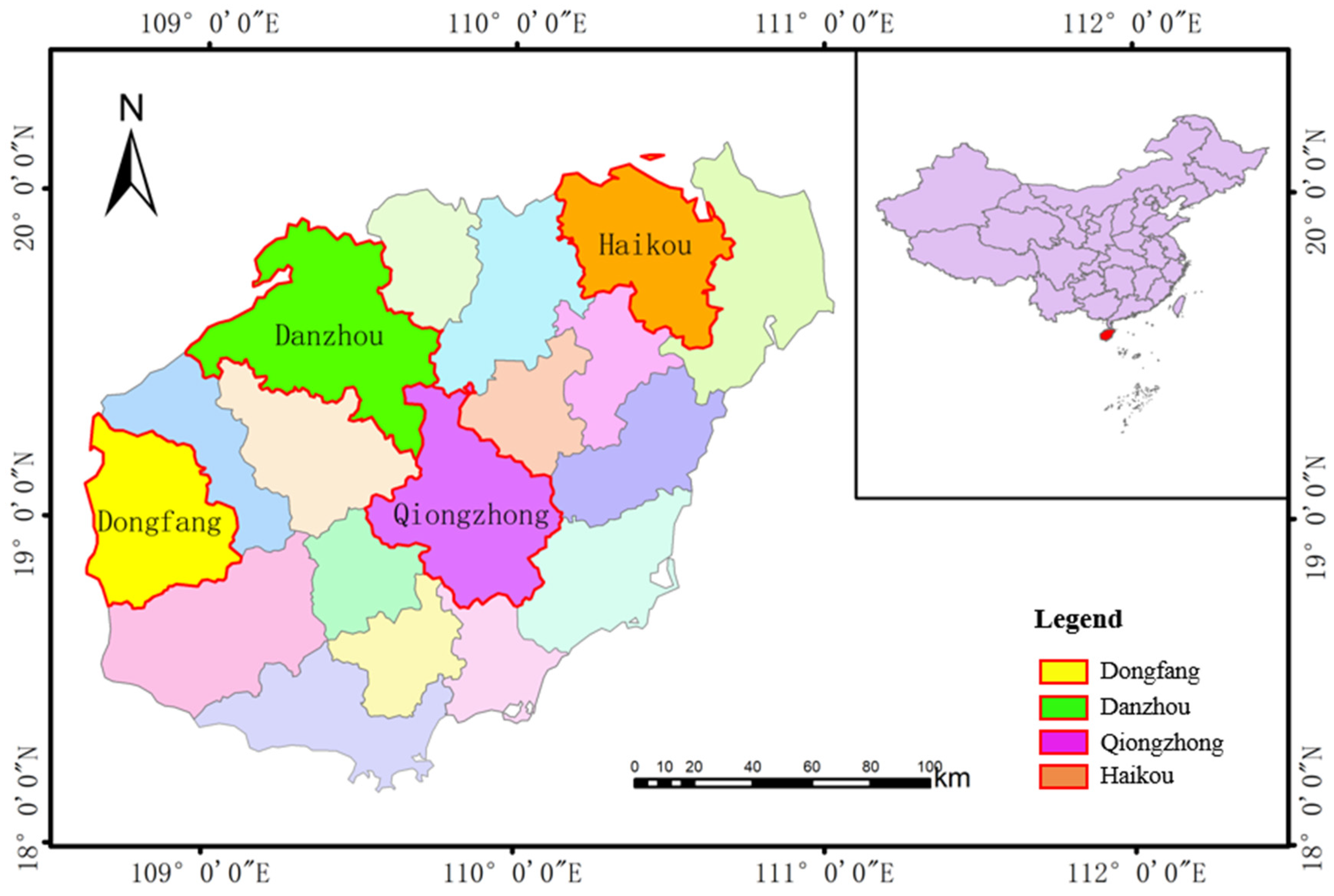
Hainan Province is located in the southernmost part of China, with geographical coordinates ranging from 18°10′ to 20°10′ N and 108°37′ to 111°03′ E, covering a total area of approximately 33,900 square kilometers. The region has a tropical monsoon marine climate, with an average annual temperature of 22.5–25.6 °C and annual precipitation generally between 1500 and 2500 mm. The western coastal areas receive less rainfall, about 1000 mm, with rainfall concentrated mainly in the summer. This study utilizes monthly rainfall data from four meteorological stations: Haikou (59758), Dongfang (59838), Danzhou (59845), and Qiongzhong (59849), spanning 252 months from January 1999 to December 2019. The selection of these four stations was deliberate, designed to capture the primary precipitation modalities across Hainan Island, spanning coastal to inland areas and humid to semi-arid regimes, thereby providing a robust test for the proposed model. Haikou represents the northern coastal area, significantly influenced by the East Asian monsoon and tropical cyclones. Dongfang represents the western dry-hot zone, situated on the leeward slope with relatively low annual precipitation, serving as a key site for testing the model’s performance in arid conditions. Danzhou represents the northwestern region, characterized by a transitional climate between coastal and inland areas. Qiongzhong represents the central mountainous area, where notable orographic uplift effects make it one of the precipitation centers of the island. This “North–West–Northwest–Central” spatial arrangement (as shown in Figure 1) enables the samples to capture the primary precipitation modalities of Hainan Island, and the specific characteristics of each station provide a basis for evaluating the model’s adaptability under different climatic conditions. The data were obtained from the National Meteorological Science Data Center (http://data.cma.cn, accessed on 12 December 2024). To evaluate model performance, the data from each station were divided sequentially into a training set and a testing set, with the training set containing the first 80% of the data and the testing set the remaining 20%.

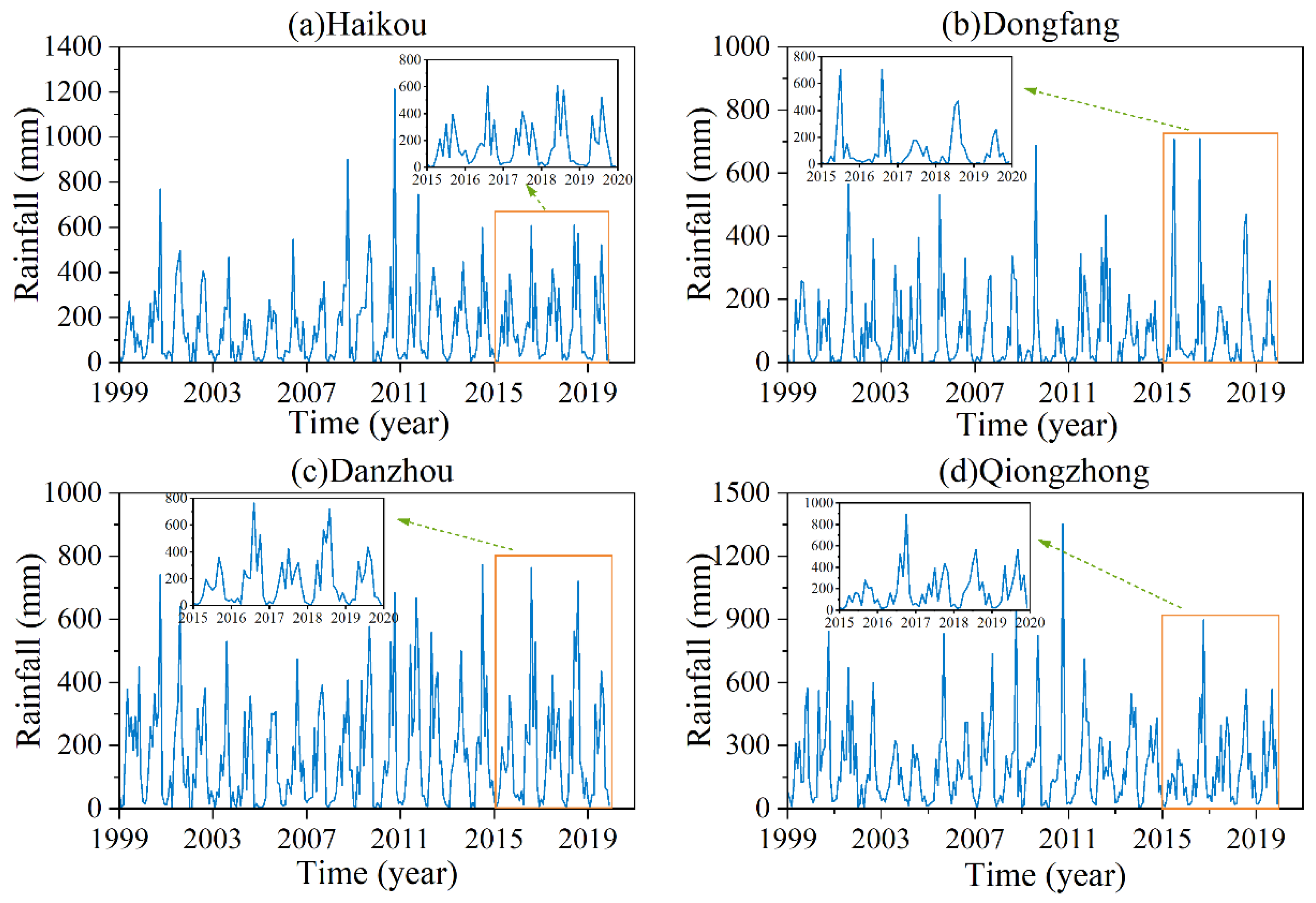
The time series of monthly rainfall at each station is shown in Figure 2, and the corresponding descriptive statistics are presented in

Table 1. The Descriptive Statistics of the rainfall data.

Site	Periods	Minimum (mm)	Maximum (mm)	Mean (mm)	Standard Deviation (mm)	Coefficient of Variation
Haikou (59758)	Training	0.0	1212.9	153.3	171.4	1.12
	Testing	9.6	610.9	163.7	166.0	1.01
Dongfang (59838)	Training	0.0	708.0	89.8	123.9	1.38
	Testing	0.0	709.6	93.2	137.3	1.47
Danzhou (59845)	Training	0.0	773.3	163.1	163.7	1.00
	Testing	3.4	764.3	187.1	189.4	1.01
Qiongzhong (59849)	Training	0.5	1353.8	196.1	194.8	0.99
	Testing	19.1	898.5	198.7	186.4	0.94

. It can be observed that the statistical characteristics of the training and testing periods are generally consistent across stations, indicating a reasonable division of the dataset. This ensures that the model built during the training period can be effectively applied to the testing period for prediction.

3. Methods

This section details the hypothesis tests and data preprocessing methods used, reviews the fundamentals of the LSTAR and GARCH models, describes the process for point and interval forecasting using the LSTAR-GARCH model, and finally outlines the model performance evaluation metrics.

3.1. Hypothesis Testing

Before constructing the model, it is essential to perform the KPSS test [24], the BDS test [20], and a skewness test to examine the non-stationarity, nonlinearity, and skewness of the monthly precipitation series. The KPSS test assumes under the null hypothesis that the time series is stationary. The BDS test assumes, under the null hypothesis, that the data are linear. The skewness test evaluates whether the time series follows a normal distribution. For detailed descriptions of the KPSS and BDS tests, please refer to Shin et al. [24] and Brock et al. [20], respectively. The skewness test assesses normality by calculating the skewness coefficient of the distribution.

3.2. Data Partitioning and Transformation

The complete dataset was divided into a training set $X_T\left(t\right)\left(t=\mathrm{1,2},\dots ,T\right)$ and a testing set $X_t\left(t\right)\left(t=T+1,T+2,\dots ,N\right)$. If the time series exhibits skewness, a Box–Cox transformation is applied to the training set prior to modeling to approximate a Gaussian distribution. The Box–Cox transformation is defined as:

$$z_t=\left\{\begin{array}{c}{\displaystyle \frac{y_t^{\lambda }-1}{\lambda }}, \lambda \ne 0\hfill \\ \log \left(y_t\right),\lambda =0\hfill \end{array}\right.$$

(1)

where $y_t$ is the original variable, $z_t$ is the transformed variable, and $\lambda$ is the Box–Cox coefficient.

Applying Equation (1) yields the transformed training set $X_T^{BC}\left(t\right)\left(t=\mathrm{1,2},\dots ,N\right)$.

3.3. The STAR Model

In the TAR model, regime switching occurs when a threshold variable exceeds or falls below a certain threshold. This switching is discontinuous. If the discontinuity at the threshold is replaced by a smooth function, the TAR model becomes a STAR model. Terasvirta [12] systematically described the modeling strategy and application procedure for STAR models. The STAR model introduces a transition function to smooth the regime switching. This study employs a two-regime STAR model, as this configuration is generally sufficient to capture the nonlinear characteristics, such as regime switching, in most practical hydrological applications. For rainfall time series, the two regimes can correspond to “low-rainfall” and “high-rainfall” states, effectively capturing the smooth transition between dry and wet periods. From a theoretical perspective, Terasvirta [12] demonstrated that the two-regime STAR model generally performs well in fitting hydro-meteorological data, while avoiding the over-parameterization and estimation complexities associated with multi-regime models. A two-regime STAR(p) model can be expressed as:

$$\begin{array}{c}{y}_t=\left({\phi }_{10}+{\phi }_{11}{y}_{t-1}+\dots +{\phi }_{1p}{y}_{t-p}\right)\left(1-G\left(s_t;\gamma ,c\right)\right)\\ +\left({\phi }_{20}+{\phi }_{21}{y}_{t-1}+\dots +{\phi }_{2p}{y}_{t-p}\right)G\left(s_t;\gamma ,c\right)+{\epsilon }_t\end{array}$$

(2)

where ${\left({\phi }_{10},{\phi }_{11},\dots ,{\phi }_{1p}\right)}^{\prime }$ and ${\left({\phi }_{20},{\phi }_{21},\dots ,{\phi }_{2p}\right)}^{\prime }$ are the autoregressive coefficients of the first and second regimes, respectively. ${\epsilon }_t$ is the residual series, $G\left(s_t;\gamma ,c\right)$ is the transition function, bounded between 0 and 1, $s_t$ is the transition variable, $\gamma$ is the smoothness parameter, and $c$ is the threshold parameter.

Alternatively, the two-regime STAR(p) model can be written as:

$$y_t=\left({\phi }_{10}+{\phi }_{11}{y}_{t-1}+\dots +{\phi }_{1p}{y}_{t-p}\right)+\left({\theta }_{20}+{\theta }_{21}{y}_{t-1}+\dots +{\theta }_{2p}{y}_{t-p}\right)G\left(s_t;\gamma ,c\right)+{\epsilon }_t$$

(3)

where ${\theta }_{2j}={\phi }_{2j}-{\phi }_{1j},{\phi }_{1j}\ne {\phi }_{2j},j=\mathrm{0,1},2,\dots ,p$.

Different forms of the transition function correspond to different regime-switching behaviors. The two most common are the logistic function (Equation (4)) and the exponential function (Equation (5)), leading to LSTAR and ESTAR models, respectively.

$$G{\left(s_t;\gamma ,c\right)}^L={\left(1+exp\left\{-\gamma \left(s_t-c\right)\right\}\right)}^{-1},\gamma >0$$

(4)

$$G{\left(s_t;\gamma ,c\right)}^E=1-exp\left\{-\gamma {\left(s_t-c\right)}^2\right\},\gamma >0$$

(5)

The STAR model employs an auxiliary regression for the linearity test to determine the transition variable $s_t$ and the transition function $G\left(s_t;\gamma ,c\right)$.

Additionally, the lag order $p$ of the STAR model is determined by the Akaike Information Criterion (AIC):

$${AIC}_p=nln\left({\sigma }^2\right)+2p$$

(6)

where $n$ and $\sigma$ are the length of the data and the error variance, respectively.

The parameters $\widehat{\rho }=\left({\phi }_{1j}^{\prime },{\phi }_{2j}^{\prime },\gamma ,c\right)$ of the STAR model can be estimated using nonlinear least squares:

$$\widehat{\rho }={\mathrm{a}\mathrm{r}\mathrm{g}\mathrm{m}\mathrm{i}\mathrm{n}}_{\rho }\underset{t=1}{\sum ^n}{\left[y_t-F\left(x_t;\rho \right)\right]}^2$$

(7)

where $F\left(x_t;\rho \right)=\left({\phi }_{10}+{\phi }_{11}{y}_{t-1}+\dots +{\phi }_{1p}{y}_{t-p}\right)\left(1-G\left(s_t;\gamma ,c\right)\right)+\left({\phi }_{20}+{\phi }_{21}{y}_{t-1}+\dots +{\phi }_{2p}{y}_{t-p}\right)G\left(s_t;\gamma ,c\right)$.

A STAR model was fitted to the transformed training set $X_T^{BC}\left(t\right)\left(t=\mathrm{1,2},\dots ,N\right)$, producing simulated values $X_T^{BCf}\left(t\right)\left(t=\mathrm{1,2},\dots ,N\right)$. The residuals $e_T^{BC}\left(t\right)\left(t=\mathrm{1,2},\dots ,N\right)$ are calculated as:

$$e_T^{BC}\left(t\right)=X_T^{BCf}\left(t\right)-X_T^{BC}\left(t\right)\left(t=\mathrm{1,2},\dots ,N\right)$$

(8)

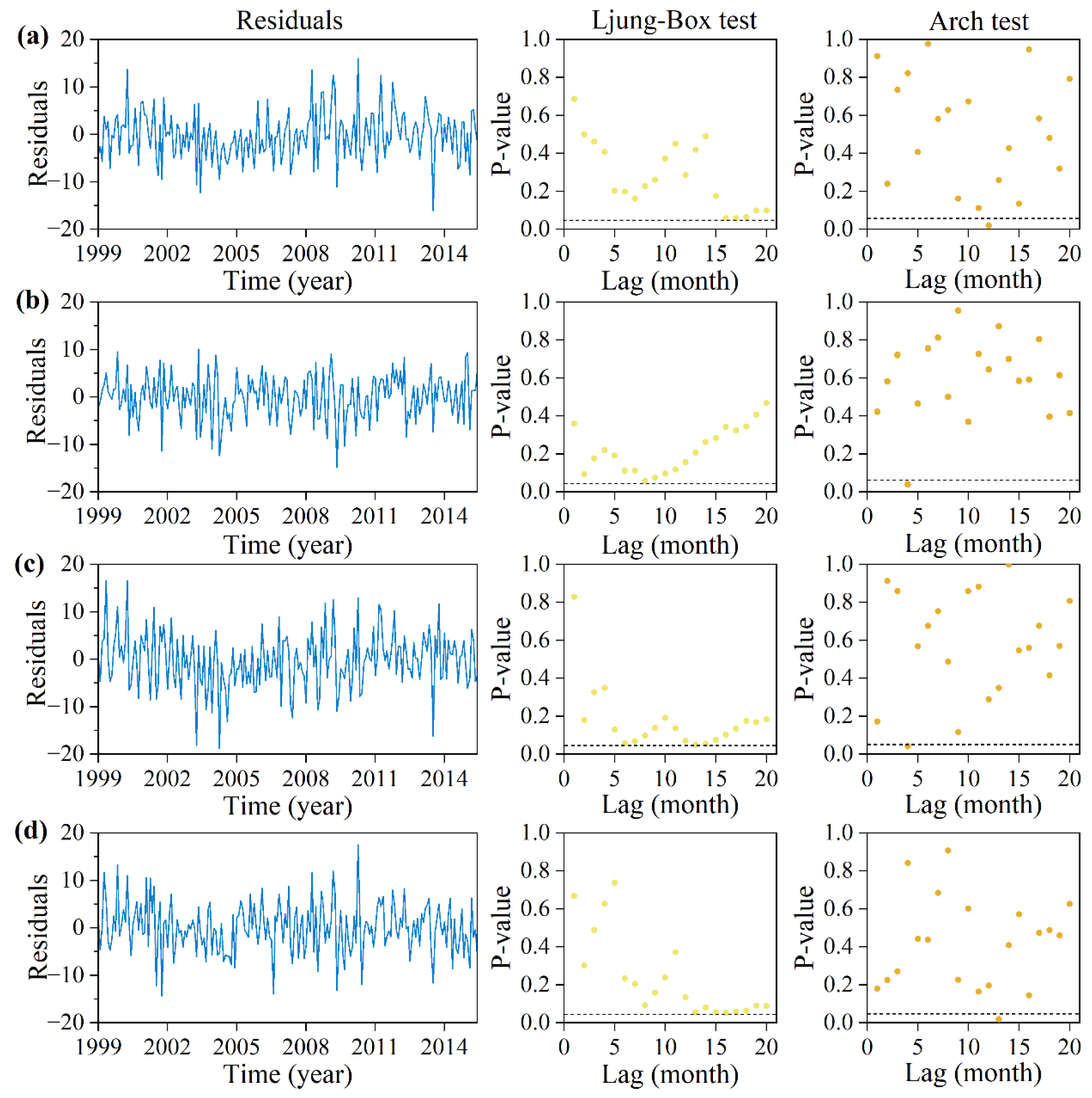
To validate the STAR model, the Ljung–Box test [25] was used to check the independence of the residuals. The null hypothesis of the Ljung–Box test is that the series is serially uncorrelated.

3.4. The GARCH Model

The GARCH$(p,q)$ model creates the conditional variance, ${\sigma }_t^2$, by a linear combination of $p$ past squared returns, ${\epsilon }_{t-i}^2(i=\mathrm{1,2},\dots ,p)$, and the $q$ previous conditional variance, ${\sigma }_{t-j}^2(j=\mathrm{1,2},\dots ,q)$, which can be specified as follows:

$${\sigma }_t^2={\alpha }_0+\underset{i=1}{\sum ^p}{\alpha }_i{\epsilon }_{t-i}^2+\underset{j=1}{\sum ^q}{\beta }_j{\sigma }_{t-j}^2$$

(9)

$${\epsilon }_t={\sigma }_t{e}_t\begin{array}{cc}& e_t~N\left(\mathrm{0,1}\right)\end{array}$$

(10)

where ${\alpha }_0$ is a constant, and ${\alpha }_i\left(i\in \left\{\mathrm{1,2},\dots ,p\right\}\right)$ and ${\beta }_j\left(j\in \left\{\mathrm{1,2},\dots ,q\right\}\right)$ are the coefficients of the GARCH$(p,q)$ model.

For the GARCH model, the orders were determined by minimizing the AIC and the parameter vector $\theta =\left({\alpha }_0,{\alpha }_i,{\beta }_j\right)$ was estimated by maximizing the log likelihood function:

$$l\left(\theta \right)=-{\displaystyle \frac{n}{2}}\log \left(2\pi \right)-{\displaystyle \frac{1}{2}}\log \left({\sigma }_{t-1\left|t-2\right.}^2+{\epsilon }_t^2/{\sigma }_{t\left|t-1\right.}^2\right)$$

(11)

To solve Equation (11), a BHHH [26] iterative method is called for:

$${\theta }^{\left(i+1\right)}={\theta }^{\left(i\right)}+{\lambda }_i{\left({\sum }_{t=1}^T{\displaystyle \frac{\partial l_t}{\partial \theta }}{\displaystyle \frac{\partial l_t}{\partial {\theta }^{\mathrm{\prime }}}}\right)}^{-1}{\sum }_{t=1}^T{\displaystyle \frac{\partial l_t}{\partial \theta }}$$

(12)

where ${\theta }^{\left(i+1\right)}$ is the estimate of $\theta$ in the $i$th iteration, and ${\lambda }_i$ is a step length. The first- and second-order derivatives of the $l\left(\theta \right)$ with respect to $\theta$. The more detailed introduction of parameter estimation in the GARCH model can be referred to Bollerslev [20]. Engle [27]. Note that (a) ${\alpha }_0>0$, ${\alpha }_i>0\left(i\in \left\{\mathrm{1,2},, \dots ,p\right\}\right)$ and ${\beta }_j>0\left(j\in \left\{\mathrm{1,2},, \dots ,q\right\}\right)$ guarantee that the conditional variance of GARCH$(p,q)$ is always positive, and (b) ${\sum }_{i=1}^p{\alpha }_i+{\sum }_{j=1}^q{\beta }_j<1$ suffices for wide-sense stationarity.

To ensure the residual series exhibits independent and identically distributed behavior, the ARCH test was applied to the residuals of the LSTAR model to detect ARCH effects. The null hypothesis of the ARCH test is that no ARCH effects are present. If ARCH effects are found, a GARCH model is established to eliminate these effects and estimate the time-varying conditional variance, ${\sigma }_t^2\left(t=\mathrm{1,2},\dots ,T\right)$. The residuals of the newly built LSTAR-GARCH model should be tested again for ARCH effects to ensure they are eliminated.

3.5. Model Forecasting

A one-step-ahead forecasting strategy was employed for the testing period. First, the fitted LSTAR-GARCH model was used to obtain the forecast mean, $X_t^{BCf}\left(t\right)\left(t=T+1,T+2,\dots ,N\right)$, and forecast variance, ${\sigma }_t^2\left(t=T+1,T+2,\dots ,N\right)$, for the transformed testing data. These were then transformed back to the original scale using the inverse Box–Cox transformation to obtain the final forecasts, $X_t^f\left(t\right)\left(t=T+1,T+2,\dots ,N\right)$.

In addition to point forecasts, interval forecasts were constructed using symmetric probability intervals, $\left[F_{\alpha /2},F_{1-\alpha /2}\right]$. At the 95% confidence level, the upper and lower forecast bounds, $X_{up}\left(t\right)$ and $X_{low}\left(t\right)$, are given by:

$$X_{up}\left(t\right)=X^f\left(t\right)+F_{0.975}\left(t\right)$$

(13)

$$X_{low}\left(t\right)=X^f\left(t\right)+F_{0.025}\left(t\right)$$

(14)

where $F_{0.025}$ and $F_{0.975}$ are the 2.5% and 97.5% quantiles of the cumulative distribution function (CDF), respectively.

For the LSTAR-GARCH model, the intervals are based on the residuals. $F_{0.025}$ and $F_{0.975}$ are calculated as:

$$F_{0.975}\left(t\right)=1.96·{\sigma }_t$$

(15)

$$F_{0.025}\left(t\right)=-1.96·{\sigma }_t$$

(16)

3.6. Model Performance Evaluation

3.6.1. Deterministic Forecast Evaluation Metrics

The Relative Error (RE) and Nash-Sutcliffe Efficiency (NSE) coefficient were selected as evaluation metrics for deterministic forecast accuracy. They are calculated as follows:

$$RE={\displaystyle \frac{1}{T}}\underset{t=1}{\sum ^T}\left|{\displaystyle \frac{X\left(t\right)-X^f\left(t\right)}{X\left(t\right)}}\right|$$

(17)

$$NSE=1-{\displaystyle \frac{{\displaystyle \sum _{t=1}^T}{\left(X\left(t\right)-X^f\left(t\right)\right)}^2}{{\displaystyle \sum _{t=1}^T}{\left(\mathrm{X}\left(t\right)-\overline{X}\right)}^2}}$$

(18)

where $T$ is the series length, $X\left(t\right)$ is the observed value, $X^f\left(t\right)$ is the forecasted value, and $\overline{X}$ is the mean of the observed series.

3.6.2. Probabilistic Interval Forecast Evaluation Metrics

The Coverage Rate (CR) and Average Relative Interval Width (Average Relative Interval Width, RIW) were selected as evaluation metrics for probabilistic interval forecasts. They are calculated as follows:

$$RIW={\displaystyle \frac{1}{T}}\underset{t=1}{\sum ^T}\left({\displaystyle \frac{X^u\left(t\right)-X^l\left(t\right)}{X\left(t\right)}}\right)$$

(19)

$$CR={\displaystyle \frac{1}{T}}\underset{t=1}{\sum ^T}\left\{X^l\left(t\right)\le X^f\left(t\right)\le X^u\left(t\right)\right\}$$

(20)

where $T$ is the series length, $X\left(t\right)$ is the observed value, $X^l\left(t\right)$ and $X^u\left(t\right)$ are the lower and upper bounds of the prediction interval, respectively.

4. Results

4.1. LSTAR-GARCH Model Construction

Before model building, a series of hypothesis tests were conducted on the monthly rainfall series.

Table 2. The skewness value of the rainfall series, the p-value of the KPSS test, and the BDS test.

Site	KPSS	BDS	Skewness
Haikou (59758)	0.100	0.000	2.179
Dongfang (59838)	0.100	0.000	2.377
Danzhou (59845)	0.100	0.000	1.346
Qiongzhong (59849)	0.100	0.000	2.080

presents the results of the KPSS test, BDS test, and skewness test. The results indicate that the monthly rainfall series at all stations are non-stationary and nonlinear at the 10% significance level, justifying the use of a nonlinear transition model. All station data also showed skewed distributions, necessitating a Box–Cox transformation prior to modeling. The skewness values presented in

Table 3. Skewness values after Box–Cox transformation for each station.

	Haikou (59758)	Dongfang (59838)	Danzhou (59845)	Qiongzhong (59849)
Skewness	−0.029	−0.158	−0.108	0.005

demonstrate that the data approximate normality post-Box–Cox transformation.

After the linearity test, a two-regime STAR model with a logistic transition function was chosen. Through parameter estimation, the most appropriate LSTAR model was selected for each station. For Haikou station, a LSTAR(6) model was built with the transition function $G{\left(x_{t-1};0.89,12.10\right)}^L$. For Dongfang station, a LSTAR(6) model was built with $G{\left(x_{t-1};524.82,11.13\right)}^L$. For Danzhou station, a LSTAR(6) model was built with $G{\left(x_{t-2};2.31,10.56\right)}^L$. For Qiongzhong station, a LSTAR(6) model was built with $G{\left(x_{t-1};0.93,25.45\right)}^L$.

After model construction, the residuals were examined. Figure 3 shows the residuals of the LSTAR model and the results of the Ljung–Box test. All p-values for the Ljung–Box test were greater than the significance level (a = 0.05; second column of Figure 3), indicating that the null hypothesis of residual independence cannot be rejected at the 0.05 level. This suggests no significant autocorrelation in the residuals, confirming the LSTAR model’s good fit to the monthly rainfall data at each station.

Before introducing the GARCH model, the presence of heteroskedasticity in the residuals needed to be verified. Figure 3 shows the residual series and the results of the ARCH effect test. The first column of Figure 4 reveals obvious volatility clustering in the residuals. The ARCH test results (third column 3 of Figure 3) show p-values below 0.05 at some lags, leading to the rejection of the null hypothesis of “no ARCH effects”. This confirms the presence of conditional heteroskedasticity in the residuals, justifying the need for a GARCH model to further characterize the volatility of the residual series.

To further capture the volatility characteristics of the residual series, a GARCH(1,1) model was fitted to the residuals of the LSTAR model for each station. To verify that the newly constructed LSTAR-GARCH model effectively eliminated conditional heteroskedasticity, the new residuals were tested again for ARCH effects. The results, shown in Figure 4, indicate that all p-values from the ARCH test are greater than the significance level (a = 0.05), suggesting that the new residual series no longer exhibits significant ARCH effects. Therefore, the constructed LSTAR-GARCH model is considered reasonable and effective.

4.2. Model Evaluation

In this section, the point and interval forecast performance of the LSTAR-GARCH model is evaluated based on the criteria established in Section 3. To clarify model performance, the results of the SVR model, SVR-GARCH model, LSTAR model, and LSTAR-ARCH model were compared. Figure 5 displays time series plots, scatter plots, and interval width plots for the point and interval forecasts during the testing period.

Table 4. Evaluation standard values and interval evaluation index change rate values for each model of the monthly rainfall series at each station.

Site	Point Forecasting			Interval Forecasting
	Model	RE	NSE	Model	RIW	ROC (%)	CR (%)	ROC (%)
Haikou (59758)	SVR	0.958	0.681	—	—	—	—	—
	SVR-GARCH	0.958	0.681	—	—	—	—	—
	LSTAR	0.756	0.802	LSTAR-GARCH	0.068	79.01	97.9	2.14
	LSTAR-GARCH	0.756	0.802	LSTAR-ARCH	5.441		100
Dongfang (59838)	SVR	1.531	0.423	—	—	—	—	—
	SVR-GARCH	1.531	0.423	—	—	—	—	—
	LSTAR	0.998	0.565	LSTAR-GARCH	0.130	62.38	93.8	4.37
	LSTAR-GARCH	0.998	0.565	LSTAR-ARCH	8.240		97.9
Danzhou (59845)	SVR	1.210	0.718	—	—	—	—	—
	SVR-GARCH	1.210	0.718	—	—	—	—	—
	LSTAR	0.969	0.774	LSTAR-GARCH	0.085	66.66	93.8	6.61
	LSTAR-GARCH	0.969	0.774	LSTAR-ARCH	5.751		100
Qiongzhong (59849)	SVR	1.024	0.631	—	—	—	—	—
	SVR-GARCH	1.024	0.631	—	—	—	—	—
	LSTAR	0.984	0.768	LSTAR-GARCH	0.065	68.97	93.8	4.37
	LSTAR-GARCH	0.984	0.768	LSTAR-ARCH	4.548		97.9

provides the numerical values of the evaluation metrics for the monthly rainfall models at each station during the testing period.

For point forecasting, the results in Table 4 show that the LSTAR and LSTAR-GARCH models achieve smaller RE values and larger NSE values compared to the SVR and SVR-GARCH models, indicating higher prediction accuracy of the LSTAR-type models, which perform comparably to or better than the modern benchmark SVR approach. It is noteworthy that the RE and NSE values are identical between SVR and SVR-GARCH, as well as between LSTAR and LSTAR-GARCH at all stations, suggesting that the GARCH component does not improve the point forecast performance of either base model for monthly precipitation data. To further verify the statistical significance of the differences between models, the Diebold-Mariano (DM) test was conducted.

Table 5. Diebold-Mariano (DM) test statistics for each station.

Site	SVR/ LSTAR	LSTAR/ LSTAR-GARCH	SVR/ SVR-GARCH	SVR/ LSTAR-GARCH	LSTAR/ SVR-GARCH	Z $(\mathit{\alpha }=0.05)$
Haikou (59758)	0.409	0.000	0.000	0.409	−0.409	$\pm 1.96$
Dongfang (59838)	0.303	0.000	0.000	0.303	−0.303	$\pm 1.96$
Danzhou (59845)	0.278	0.000	0.000	0.278	−0.278	$\pm 1.96$
Qiongzhong (59849)	0.788	0.000	0.000	0.788	−0.788	$\pm 1.96$

provides the Diebold-Mariano (DM) test statistics for the monthly rainfall models at each station during the testing period. The DM test results show that the absolute values of the test statistics for comparisons between LSTAR-type and SVR-type models (e.g., SVR vs. LSTAR) are all below the critical value of 1.96, confirming that the LSTAR-type models do not significantly outperform the SVR-type models at any station; however, they consistently show a slight numerical advantage in the test statistics. Furthermore, comparisons within each model type reveal that the GARCH specification provides no enhancement in point forecast accuracy. Together, these findings strengthen the reliability of the model comparison conclusions. Further analysis reveals that the LSTAR model achieved NSE values above 0.75 and generally low RE values at all stations except Dongfang, indicating good predictive performance at Haikou, Danzhou, and Qiongzhong stations, but weaker performance at Dongfang. Figure 4 further reveals a consistent systematic bias across all stations for the LSTAR model: low precipitation values were overestimated, while high precipitation values were underestimated. This bias was particularly pronounced at Dongfang station, explaining its lower predictive accuracy. Given that the point forecast evaluation metrics for the LSTAR and LSTAR-GARCH models are identical, only the point forecasting results of the LSTAR model are shown in Figure 5.

For interval forecasting, due to the better point prediction accuracy of LSTAR models, this model is chosen for interval prediction. The performance of the LSTAR-ARCH and LSTAR-GARCH models was compared. Table 4 shows that all models achieved CR values above 90% at all stations, indicating high reliability. Although the LSTAR-GARCH model had slightly lower CR values than the LSTAR-ARCH model at each station, the difference was minimal, with only a few individual data points not covered. However, the average RIW of the LSTAR-ARCH model was significantly larger than that of the LSTAR-GARCH model (e.g., 8.240 vs. 0.130 at Dongfang station). This indicates that while the LSTAR-ARCH model has high coverage, its prediction intervals are overly conservative and imprecise. In contrast, the LSTAR-GARCH model provides narrower and more practical rainfall intervals while maintaining high coverage, demonstrating its ability to more effectively characterize uncertainty in the rainfall series. Considering both metrics, the LSTAR-GARCH model outperforms the LSTAR-ARCH model at all stations.

5. Discussions

This study constructed a hybrid LSTAR-GARCH model for point and interval forecasting of monthly rainfall series at four stations in Hainan Province and compared it with the LSTAR and LSTAR-ARCH models. The results show that the hybrid model performed excellently in interval forecasting but did not significantly outperform the standalone LSTAR model in point forecasting. The findings are discussed below in the context of relevant domestic and international research.

First, the point forecast results show that the LSTAR model achieved high NSE values (>0.75) at three stations (excluding Dongfang), indicating its ability to effectively capture the nonlinear characteristics of the rainfall series. This aligns with the conclusions of Teräsvirta [12] and Saha et al. [16], who found that STAR-type models have advantages in handling regime-switching time series. The poorer performance at Dongfang station can be attributed to its unique climatic and geographic conditions: located on the western leeward coast of Hainan, it lies in a rain shadow area with relatively low annual precipitation and is strongly influenced by the dry and hot foehn effect from the central mountains. Additionally, rainfall in this region is more susceptible to localized convective systems and tropical cyclone remnants, which are highly stochastic and less periodic, making them harder to capture with a univariate time-series model. These factors likely introduce higher unpredictability and structural breaks that the LSTAR model could not fully accommodate. This finding does not diminish the value of the model but rather provides a more precise delineation of its generalizability and a clearer evolution path for its application. Furthermore, the proposed framework demonstrates direct potential for generalization in typical tropical humid monsoon regions.

Notably, incorporating the GARCH model did not improve point forecast accuracy, consistent with some previous findings (e.g., Guo et al. [19]). A possible reason is that while rainfall series exhibit volatility, it has minimal impact on the conditional mean. Since GARCH primarily models the conditional variance, its contribution to point forecast accuracy is limited. This suggests that for point forecasting tasks, optimization should focus more on the mean model. To prove this explanation more formally, we make the following simple proof.

Considering a simplest STAR (1) model for representing Equation (2), the conditional mean of $X_t$ of the t-th time point, conditioned upon $X_{t-1}$ of the $t-$1-th time point, can be obtained by the following:

$$\begin{array}{c}E\left(X_t|X_{t-1}\right)=E\left[{\phi }_{10}\left(1-G\left(s_t;\gamma ,c\right)\right)\right]+E\left[{\phi }_{11}{y}_{t-1}\left(1-G\left(s_t;\gamma ,c\right)\right)\right]\\ +E\left[{\phi }_{20}G\left(s_t;\gamma ,c\right)\right]+E\left[{\phi }_{21}{y}_{t-1}G\left(s_t;\gamma ,c\right)\right]+E\left({\epsilon }_t\right)\end{array}$$

(21)

From Equation (10), ${\epsilon }_t$ is an independent random variable with mean 0 and time-varying variance ${\sigma }_t^2$. Therefore, the conditional mean can be expressed as follows:

$$E\left(X_t|X_{t-1}\right)={\phi }_{10}\left(1-G\left(s_t;\gamma ,c\right)\right)+{\phi }_{11}{y}_{t-1}\left(1-G\left(s_t;\gamma ,c\right)\right)+{\phi }_{20}G\left(s_t;\gamma ,c\right)+{\phi }_{21}{y}_{t-1}G\left(s_t;\gamma ,c\right)$$

(22)

From Equation (22), the conditional mean is independent of the ${\epsilon }_t$. Form Equation (9), ${\epsilon }_t$ is dependent on the ${\sigma }_t^2$ that is estimated by GARCH models. Thus, the conditional mean is independent of GARCH models. That is to say, GARCH models do not have any influence on the simulation and prediction of mean value behavior.

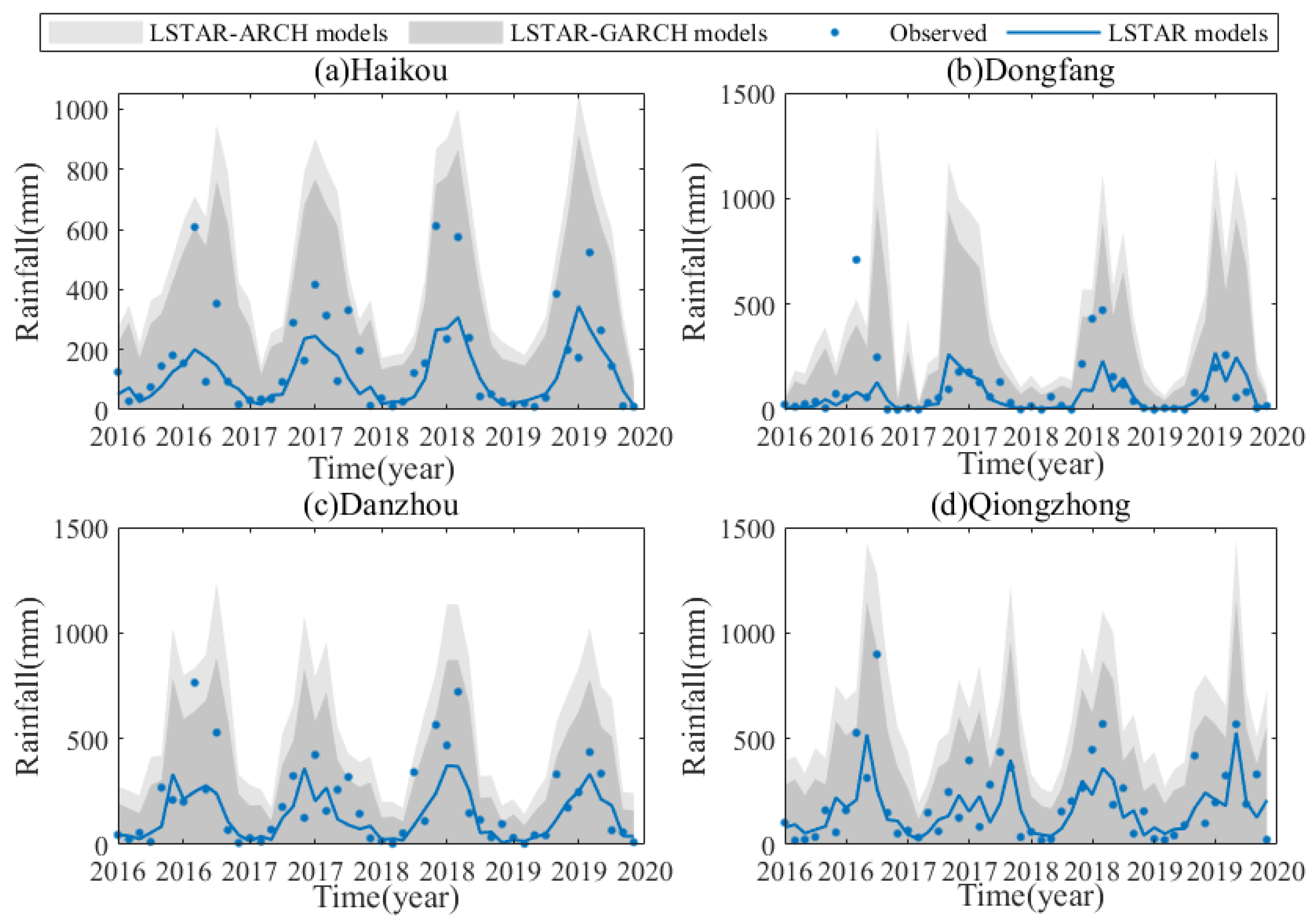
In terms of interval forecasting, the LSTAR-GARCH model demonstrated high coverage rates (CR > 93%) and narrower relative interval widths (RIW) across all stations, significantly outperforming the LSTAR-ARCH model. This indicates that the GARCH model more effectively captures the volatility clustering in the residuals, leading to more precise prediction intervals. This result is consistent with the findings of Guo et al. [19] in runoff forecasting, further validating the potential of GARCH-type models to improve uncertainty quantification in hydro-meteorological variables. Regarding the magnitude of the Relative Interval Width (RIW) obtained from the LSTAR-GARCH model (ranging from 0.065 to 0.130), it is important to justify its reasonability from both methodological and practical perspectives. First, the RIW is a normalized metric calculated as the average ratio of the interval width to the actual observed rainfall. During dry seasons or at stations with lower mean rainfall (e.g., Dongfang), even a modest absolute interval width can result in a larger RIW value, as the denominator (observed rainfall) is small. Second, and more fundamentally, monthly rainfall in tropical monsoonal regions like Hainan is characterized by high volatility and a pronounced heavy-tailed distribution. The presence of extreme rainfall events necessitates sufficiently wide prediction intervals to reliably encapsulate the inherent and substantial uncertainty. The primary objective of interval forecasting is to achieve a high Coverage Rate (CR), and our model successfully maintains CRs between 93.8% and 97.9% at the 95% confidence level. The resultant RIW values are a direct and honest reflection of the uncertainty required to attain this reliable coverage, representing a rational trade-off between precision and reliability. Therefore, the RIWs generated by the LSTAR-GARCH model are not only justifiable but also demonstrate its capability to effectively quantify the true variability in rainfall series.

Nevertheless, this study has some limitations. First, it used data from only four stations, limiting the sample representativeness. Second, the selection of transition variables and lag orders still relied on traditional methods; future work could incorporate machine learning techniques for automatic optimization. Additionally, external variables (e.g., ENSO, monsoon indices) were not considered, which could be an important direction for improving model performance. To address these limitations, future research should focus on the following directions: (1) Embedding physical mechanisms: Introducing exogenous strong signals such as sea surface temperature, wind fields, and humidity as transition variables or input features to enhance the physical consistency and predictive capability of the model in complex regions; (2) Spatially explicit modeling: Developing parameterized spatiotemporal STAR models to characterize the spatial heterogeneity of nonlinear precipitation dynamics in the form of continuous fields; (3) Hybrid framework integration: Exploring hybrid modeling approaches that combine the current framework with machine learning algorithms to overcome the limitations of a single model framework in addressing diverse climatic characteristics across entire basins.

In summary, the LSTAR-GARCH model shows promising application potential for interval forecasting of monthly rainfall, especially for series with significant heteroskedasticity. Future research could extend this model to a multivariate or spatial forecasting framework and incorporate more meteorological factors to further enhance forecast capability.

6. Conclusions

This study constructed a hybrid LSTAR-GARCH model for point and interval forecasting of monthly rainfall series and compared it with a hybrid LSTAR-ARCH model to validate the effectiveness of the LSTAR-GARCH approach. Based on the analysis of monthly rainfall data from Haikou, Dongfang, Danzhou, and Qiongzhong stations, the effectiveness of each model was evaluated, leading to the following main conclusions:

(1)

For point forecasting, the LSTAR model performed well at all stations except Dongfang. A comparison of the point forecast performance between the hybrid LSTAR-GARCH model and the standalone LSTAR model showed that the evaluation metrics were identical, indicating that the GARCH component did not enhance the modeling and predictive performance of the LSTAR model.

(2)

For interval forecasting at the 95% confidence level, compared to the LSTAR-ARCH model, the LSTAR-GARCH model produced much narrower relative interval widths while maintaining nearly identical coverage rates. Therefore, the LSTAR-GARCH model exhibits superior interval forecasting performance compared to the LSTAR-ARCH model, reducing the uncertainty of interval forecasts.

In conclusion, the results demonstrate that the LSTAR-GARCH model can achieve satisfactory point and interval forecast performance. We conclude that the GARCH model does not impact point forecasts but, when combined with the LSTAR model, yields better interval forecasting performance. Due to the non-stationary and nonlinear characteristics of hydrological series like rainfall, the model used in this study is highly recommended for other hydrological and climatic variables in changing environments. However, note that this study considered rainfall data from only four stations. Therefore, future research should consider applying these models to other study regions with different climates and backgrounds for further comparison and demonstration.