A Slope Dynamic Stability Evaluation Method Based on Variable Weight Theory and Trapezoidal Cloud Model

Abstract

Slope instability may cause severe casualties, property losses, and ecological damage. To accurately evaluate slope stability grades and mitigate geological hazards, a dynamic stability assessment method based on variable weight theory and trapezoidal cloud model is proposed. First, an evaluation index system for slope stability is established following the principles of uniqueness, purposefulness, and scientific validity. Then, to improve the accuracy of subjective constant weights, the intuitionistic fuzzy analytic hierarchy process (IFAHP) is employed to calculate subjective constant weights. Considering the contrast intensity and conflict among indicators, an improved CRITIC method is applied to determine objective constant weights. To balance subjective and objective factors and avoid constant weight imbalance, the optimal comprehensive constant weights are computed based on game theory, effectively reducing bias caused by single weighting methods. Furthermore, to fully account for the influence of indicator state values on their weights, variable weight theory is introduced to dynamically adjust the comprehensive constant weights. Finally, based on the variable weights of evaluation indicators, a trapezoidal cloud model is utilized to construct the slope stability evaluation model, which is validated through an engineering case study. The results indicate that the stability grade of Stage 1 is assessed as basically stable, while Stages 2 and 3 are evaluated as stable. Numerical simulations show the safety factors of the three stages are 1.36, 1.83, and 2.36, respectively, verifying the correctness of the proposed model. The proposed model demonstrates practical engineering value in slope stability assessment and can be referenced for slope reinforcement and hazard prevention in later stages.

1. Introduction

Slope stability evaluation is a core technique for ensuring infrastructure safety and mitigating geological disaster risks, and innovations in its theories and methods are crucial to the sustainable development of transportation engineering, mining, and urban construction [1,2]. With the large-scale advancement of engineering construction, slopes are increasingly confronted with complex geological and environmental challenges [3]. Frequent slope failures cause significant loss of life, property damage, and ecological degradation. Moreover, slope stability issues exhibit notable multi-factor coupling, spatiotemporal dynamics, and complexity of failure mechanisms. Traditional single-method approaches are increasingly inadequate for precise evaluation requirements [4,5]. Therefore, conducting scientifically accurate slope stability assessments based on multiple theories holds significant practical importance.

Numerous scholars have conducted extensive research on slope stability evaluation. Nguyen [6] simulated the effects of various rainfall scenarios on slope saturation and velocity vectors using FLAC 3D 6.0 software, finding that high-intensity, short-duration rainfall is prone to trigger slope instability, and proposed reinforcement measures combining soil nails and steel mesh, and validated that slope stability is enhanced after reinforcement. The results provide a reference for similar slope stability assessments and mitigation efforts. Chand [7] utilized UAV-acquired imagery to construct a slope surface model and generated a model with realistic geometry through numerical simulation. Applying the finite difference method and limit equilibrium method, he analyzed safety factors and failure probabilities under static, pseudo-static, and dynamic loads, providing an effective approach combining numerical simulation and probabilistic analysis for slope stability evaluation. Kumar [8] developed a numerical simulation model of slopes incorporating multiple soil layers, and analyzed variations in multiple slope parameters by simulating dry and wet conditions as well as two rainfall scenarios. The study validated the effectiveness of impermeable layers in enhancing slope stability, thereby providing a basis for waterproof design of open-pit mine slopes. However, numerical simulation methods rely on precise geological parameters and boundary conditions, and have limited adaptability to complex nonlinear problems, exhibiting drawbacks such as high computational costs and difficulties in parameter inversion, making them insufficient for the rapid assessment demands of engineering applications. In recent years, machine learning algorithms have demonstrated potential in slope stability prediction due to their strong nonlinear fitting capabilities. Pei et al. [9] proposed three knowledge-guided machine learning (KGML) methods to integrate geotechnical knowledge into data-driven models for slope stability prediction. Benchmarked against pure data-driven models and domain knowledge–based models using 96 slope cases and five-fold cross-validation, the KGML methods outperformed both, with hybrid models and knowledge-guided loss function reducing discrepancies between predictions and factor-of-safety values, aligning better with slope stability physics. Huang et al. [10] innovatively used long short-term memory (LSTM) for slope stability prediction. With Ganzhou as the study area, they selected 5 control factors, built slope models via Geo-Studio, calculated stability coefficients with limit equilibrium method, and created 2160 training and 450 testing samples, comparing LSTM with convolutional neural network (CNN), support vector machine (SVM), and random forest (RF) models via root mean square error (RMSE) and modeling efficiency (EF). LSTM extracted global features better, achieving the highest accuracy. Sabri et al. [11] presented a comparative study of four neural network-based models—artificial neural network (ANN), Bayesian neural network (BNN), CNN, and deep neural network (DNN)—for slope stability analysis. They collected soil parameters (cohesion, internal friction angle, and volumetric weight) and seismic coefficients as inputs and built a dataset of 1000 samples (800 for training, 200 for testing). They found that ANN outperformed other models in the testing phase. However, machine learning methods rely heavily on large amounts of high-quality data, exhibit a “black box” nature, and have limited interpretability regarding physical mechanisms. Their generalization capability is constrained by data distribution and parameter tuning strategies. Slope stability evaluation is inherently a complex process characterized by fuzziness and randomness, where the boundary definitions and interactions of influencing factors are often difficult to quantify precisely. Fuzzy theory provides an effective approach to address such issues through membership functions and uncertainty modeling. Chen et al. [12] proposed a group decision-making analytic hierarchy process (AHP) method based on confidence indices, which effectively addresses the issue of fixed indicator weights in rock slope stability assessment, and applied it to the stability assessment of a slope in Fujian province. The results indicate overall slope stability but local extreme instability, which is highly consistent with actual field conditions, validating the effectiveness of the proposed evaluation method. Bai et al. [13] established a risk assessment model for gently inclined mudstone bedding slopes using the analytic hierarchy process (AHP) and fuzzy comprehensive evaluation (FCE) and selected four primary evaluation indicators and 16 secondary indicators, calculated indicator weights via AHP, constructed membership functions for single and synthetic index measurement, and determined risk grades using the weighted average membership degree criterion. A case study in Guizhou showed the slope risk grade was high risk, consistent with actual monitoring data, verifying the method’s reliability and providing a new approach for slope risk assessment during the operation period. Wu et al. [14] proposed a modified cloud model for stability grade evaluation of high-steep open-pit slopes with soft rock formations. Based on the AHP, they established an evaluation index system with quantized grade intervals, calculated the weight of each index. Taking a specific open-pit mine as an example, the results showed that the slope stability was unstable, consistent with numerical simulation and traditional limit equilibrium method results, confirming the model’s scientificity and providing guidance for open-pit mine safety production. Yang et al. [15] combined fuzzy analytic hierarchy process (FAHP), information entropy theory, and set pair analysis (SPA), proposing an improved set pair analysis model (EFAHP-SPA) for open-pit mine slope stability evaluation, and validated the model’s effectiveness and reliability. These methods integrate qualitative knowledge with quantitative analysis, thereby addressing the limitations of traditional numerical simulation and machine learning in handling uncertainties. These studies have significantly contributed to the advancement of slope stability theory. However, slope stability evaluation is a complex process influenced by multiple variables and factors. Relying solely on a single theory to assign weights to evaluation indicators has inherent limitations; only dynamic weighting can reasonably reflect the varying impact of different indicators on the evaluation outcome. Moreover, effectively balancing the relationship between qualitative and quantitative indicators, as well as addressing the fuzziness and randomness between indicators and evaluation criteria intervals to scientifically determine slope stability levels, remains one of the urgent challenges.

Therefore, this study first constructed a slope stability evaluation indicator system based on indicator selection principles. Subsequently, the subjective constant weights and objective constant weights of the evaluation indicators were determined using the intuitionistic fuzzy analytic hierarchy process and an improved CRITIC method, respectively, followed by the calculation of the comprehensive constant weights of each indicator based on game theory. Meanwhile, dynamic adjustment of the comprehensive constant weights was performed by introducing variable weighting theory. Finally, based on the dynamically adjusted indicator weights, a slope stability evaluation model was established using the trapezoidal cloud model, and its validity was verified through engineering case studies. This study offers a novel approach for slope stability evaluation, while providing more reliable theoretical support and technical methods for engineering practice.

2. Study Area

The H1 landslide study area is located in Haidong City, Qinghai Province, situated on the northern bank of Ganzhan Valley at the front edge of a mid-high mountain slope, as shown in Figure 1. It is adjacent to the north side of the under-construction Jiaxi Highway, providing convenient transportation. The terrain of the region slopes from higher elevations in the north to lower elevations in the south, with altitudes ranging from 2501 to 2852 m. The landslide is classified as a medium-sized deep-seated translational slide. On 11 December 2021, a sudden slide occurred, causing damage to a transmission tower located in the middle of the slope, road fractures, and the burial of an excavator. This event directly threatened the safety of the under-construction Jiaxi Highway and the lives and properties of residents at the foot of the slope.

The rear edge of the landslide presents a steep-to-gentle transitional zone: the front part of the rear edge is steep, forming a free face, while the back part is relatively gentle. The shear outlet at the front edge is bounded by a steep scarp formed by highway excavation. The rear edge elevation is 2600 m, the front toe elevation is 2523 m, giving a slope height of 77 m and an average gradient of 27°. The plan view is irregularly “tongue-shaped,” and the cross-section is convex, with uneven variations in slope steepness. A synclinal fold structure is developed near the landslide area. The rock mass within the syncline core is fractured, and surface runoff erosion has carved a debris flow gully. The landslide mass rises about 60 m above the ground, with a triangular distribution, a flat top, and side slopes of about 1:1, covered with surface vegetation. The landslide area corresponds to an accumulation body at the mouth of a debris flow gully. The debris flow accumulation body at the gully mouth is 400~500 m wide, 20~50 m thick, composed mainly of cohesive soil mixed with gravelly soil, and classified as a large-scale dormant debris flow gully. The landslide mass developed within Quaternary colluvial, alluvial, and debris flow deposits. The lithology is dominated by gravelly soil containing sandstone fragments, with a loose structure and significant permeability variation. The rear boundary is marked by horseshoe-shaped cracks and two tiers of steep scarps. Intense deformation occurs in the middle section, and the shear outlet at the front edge is situated at the highway scarp.

Influenced by differential uplift and subsidence from regional neotectonic movements, the local terrain exhibits steep slopes that provide favorable topographic conditions for landslide formation. In particular, the exposed Quaternary strata in the landslide area are dominated by variegated gravelly soil, which is highly sensitive to changes in water content, creating a vulnerable stratigraphic background. Under rainfall conditions, especially when water infiltrates into the slope from diversion pipelines or channels, the landslide mass experiences a significant increase in water content, leading to greater self-weight of the soil. Meanwhile, infiltration and atmospheric precipitation soften the sliding surface, causing the soil within the landslide zone to approach saturation, exhibiting soft-plastic or flow-plastic states. This process alters the soil’s physical and mechanical properties, ultimately reducing slope stability and triggering the landslide disaster.

To conduct a dynamic stability evaluation of the slope, this study selects the typical cross-section 1-1’ at the landslide site for investigation and divides the process into three stages based on actual conditions: (1) Stage 1 corresponds to the natural condition of the slope, where the overall planform exhibits an irregular “tongue-shaped” morphology. Severe deformation and damage are observed on the slope surface, with multiple tensile cracks appearing in the middle and rear portions, and several bulging cracks at the front edge. After deformation, a distinct landslide scarp developed, featuring arcuate tensile cracks at the rear. On the western side of the landslide, notable tension trenches and striations formed, and these trenches nearly penetrate the western boundary. (2) Stage 2 involves reinforcement of the accumulative body through dual measures of slope cutting for unloading and sheet pile wall support. (3) Stage 3 consists of treatment of the middle and lower parts of the landslide body, where, based on the previous slope cutting and support measures, further slope cutting is implemented to achieve improved remediation effects.

3. Methodology

3.1. Construction of an Evaluation Indicator System

The evaluation of slope stability is a complex process influenced by numerous factors; therefore, it is essential to comprehensively and scientifically select the factors affecting slope stability based on the actual conditions of the slope [16,17,18,19]. Therefore, this study integrates existing relevant research, and, based on the principles of uniqueness, purposefulness, and scientific validity in indicator selection, while also taking into account the actual conditions of the slope, consulted several industry experts, and ultimately selected nine evaluation indicators, thereby constructing a slope stability evaluation indicator system, with the results shown in

Table 1. Evaluation indicator system for slope stability.

Evaluation Indicator	Unit
Rock quality index X1	%
Cohesion X2	MPa
Internal friction angle X3	°
Slope height X4	m
Maximum rainfall during event X5	mm
Stratigraphic lithology X6	/
Rock mass structural type X7	/
Impact of human engineering activities X8	/
Groundwater influence X9	/

.

3.2. Determination of Evaluation Indicator Weights

The determination of weights is a critical step in multi-indicator evaluation systems. Sole reliance on subjective methods (e.g., AHP) may introduce expert bias, while purely objective methods (e.g., entropy weight method) might neglect valuable expert experience. Furthermore, constant weights fail to reflect the dynamic impact of an indicator’s state value on the overall evaluation. To overcome these limitations, this study adopts a comprehensive weighting strategy that integrates both subjective and objective information, followed by a dynamic adjustment. Specifically, the intuitionistic fuzzy AHP (IFAHP) was chosen for subjective weighting to handle the inherent uncertainty and vagueness in expert judgments. An improved CRITIC method was employed for objective weighting to more accurately capture the contrast intensity and conflict between indicators. These two are then fused using game theory to achieve a balanced, constant weight, which is subsequently adjusted by variable weight theory based on the actual state of the evaluation object.

3.2.1. Determination of Subjective Constant Weights

To fully reflect expert knowledge and experience, the analytic hierarchy process (AHP) is commonly used to determine the subjective weights of evaluation indicators, but AHP cannot capture the fuzziness in the decision-maker’s preference toward indicators, nor can it accurately express indecision or abstention in evaluating objective matters, thus making it difficult to achieve objectivity and accuracy [20]. To overcome this limitation, the intuitionistic fuzzy analytic hierarchy process (IFAHP) is employed in this study [21]. IFAHP extends the traditional fuzzy set by introducing an additional degree of non-membership, allowing experts to express their confidence level and uncertainty in pairwise comparisons more flexibly. This provides a more robust mathematical framework to handle the imprecision inherent in subjective judgment. The subjective constant weights of evaluation indicators are determined using IFAHP so as to further improve the accuracy and applicability of weight calculation. The specific steps are as follows:

1. Construction of the intuitionistic fuzzy judgment matrix

Experts perform pairwise comparisons of the indicators using the provided scale. The results are not single values but intuitionistic fuzzy numbers, each consisting of a membership degree (μ_ij), a non-membership degree (v_ij), and a calculated hesitation degree (π_ij). This forms the intuitionistic fuzzy judgment matrix L. Pairwise comparisons of evaluation indicators are performed by experts based on the evaluation scale and its corresponding scores, and the relative importance of each indicator is determined. The evaluation scale and its corresponding scores are presented in

Table 2. Evaluation scales and corresponding scores.

Evaluation Scale	Score
Indicator i is extremely more important than j	0.9
Indicator i is strongly more important than j	0.8
Indicator i is obviously more important than j	0.7
Indicator i is slightly more important than j	0.6
Indicator i is equally important as j	0.5
Indicator j is slightly more important than i	0.4
Indicator j is obviously more important than i	0.3
Indicator j is strongly more important than i	0.2
Indicator j is extremely more important than i	0.1

.

The corresponding scores are represented by intuitionistic fuzzy numbers, and the intuitionistic fuzzy judgment matrix is constructed as shown in Equation (1).

$$L={(l_{ij})}_{M\times M}={({\mu }_{ij},v_{ij})}_{M\times M}=\left[\begin{array}{cccc}({\mu }_{11},v_{11})& ({\mu }_{12},v_{12})& \cdots & ({\mu }_{1M},v_{1M})\\ ({\mu }_{21},v_{21})& ({\mu }_{22},v_{22})& \cdots & ({\mu }_{2M},v_{2M})\\ ⋮& ⋮& \ddots & ⋮\\ ({\mu }_{M1},v_{M1})& ({\mu }_{M2},v_{M2})& \cdots & ({\mu }_{MM},v_{MM})\end{array}\right]$$

(1)

where μ_ij represents the membership degree, indicating the extent to which experts consider indicator i to be more important than j; v_ij represents the non-membership degree, indicating the extent to which indicator j is considered more important than i.

2. Consistency check

To assess the consistency in the perceived importance of each evaluation indicator and to obtain more reasonable indicator weights, a consistency check must be conducted on the intuitionistic fuzzy judgment matrix, and the specific method is described as follows [22].

(1) The consistency judgment matrix $\overline{L}={\left({\overline{l}}_{ij}\right)}_{M\times M}$ is constructed based on the intuitionistic fuzzy judgment matrix L = (l_ij)_M×M.

When j ≥ i + 2, ${\overline{l}}_{ij}=\left({\overline{\mu }}_{ij},{\overline{v}}_{ij}\right)$; when j = i + 1 or j = i, ${\overline{l}}_{ij}=l_{ij}$; and when j < i, ${\overline{l}}_{ij}=\left({\overline{\mu }}_{ij},{\overline{v}}_{ij}\right)$. Here, ${\overline{\mu }}_{ij}$ and ${\overline{v}}_{ij}$ are defined in Equations (2) and (3).

$${\overline{\mu }}_{ij}={\displaystyle \prod _{t=i+1}^{j-1}\left(\frac{{\mu }_{it}{\mu }_{tj}}{{\mu }_{it}{\mu }_{tj}+\left(1-{\mu }_{it}\right)\left(1-{\mu }_{tj}\right)}\right)}$$

(2)

$${\overline{v}}_{ij}={\displaystyle \prod _{t=i+1}^{j-1}\left(\frac{v_{it}{v}_{tj}}{v_{it}{v}_{tj}+\left(1-v_{it}\right)\left(1-v_{tj}\right)}\right)}$$

(3)

(2) The consistency threshold coefficient τ is defined, which is generally set as τ = 0.1. The distance measure between L and $\overline{L}$ is defined in Equation (4):

$$d(\overline{L},L)={\displaystyle \frac{1}{2(M-1)(M-2)}}{\displaystyle \sum _{i=1}^N{\displaystyle \sum _{j=1}^N(\left|{\overline{\mu }}_{ij}-{\mu }_{ij}\right|+\left|{\overline{v}}_{ij}-v_{ij}\right|+\left|{\overline{\pi }}_{ij}-{\pi }_{ij}\right|)}}$$

(4)

Where π_ij = 1 − μ_ij − v_ij represents the hesitation degree of experts regarding the comparison between two indicators, and the hesitation degree effectively reflects the subjective uncertainty arising when experts compare importance levels, thereby rendering the subjective weights more reasonable. If L and $\overline{L}$ satisfy $d(\overline{L},L)<\tau$, L is considered to have passed the consistency check; otherwise, when $d(\overline{L},L)\ge \tau$, L is appropriately adjusted until it passes the consistency check.

(3) Determination of Subjective Constant Weights

The intuitionistic fuzzy weight for each indicator is calculated based on the consistent judgment matrix. This weight is still an intuitionistic fuzzy number. A scoring function is then applied to convert the intuitionistic fuzzy number into a crisp value, which is finally normalized to obtain the subjective constant weight for each indicator.

The intuitionistic fuzzy weight w_j^* of the jth indicator is defined in Equation (5):

$$w_j^{*}=\left({\mu }_j^{*},v_j^{*}\right)=\left({\displaystyle \frac{{\displaystyle \sum _{i=1}^M{\mu }_{ij}}}{{\displaystyle \sum _{i=1}^M{\displaystyle \sum _{j=1}^M(1-v_{ij})}}}},1-{\displaystyle \frac{{\displaystyle \sum _{i=1}^M\left(1-{\mu }_{ij}\right)}}{{\displaystyle \sum _{i=1}^M{\displaystyle \sum _{j=1}^M{v}_{ij}}}}}\right)$$

(5)

According to the definition, the fuzzy transformation function H(j) is expressed using Equation (6):

$$H\left(j\right)={\mu }_j^{*}+{\pi }_j^{*}\left({\displaystyle \frac{{\mu }_j^{*}}{{\mu }_j^{*}+v_j^{*}}}\right)\hspace{1em}\left(j=1,2,\cdots ,M\right)$$

(6)

The subjective constant weight w_1j of the jth indicator is given by Equation (7):

$$w_{1j}={\displaystyle \frac{H\left(j\right)}{{\displaystyle \sum _{i=1}^{M}H\left(j\right)}}}$$

(7)

3.2.2. Determination of Objective Constant Weights

Objective weighting methods derive weights based solely on the intrinsic properties of the dataset, free from human subjectivity. The CRITIC (criteria importance through intercriteria correlation) method is a prominent objective method that accounts for both the contrast intensity (the amount of information an indicator carries) and the conflict (the correlation) between indicators [23]. This dual consideration makes it superior to methods that only consider variance or only correlations. However, a limitation of the standard CRITIC method is that it uses standard deviation to measure contrast intensity. Standard deviation is an absolute measure of dispersion and is highly sensitive to the units and scale of different indicators, which can lead to bias when evaluating indicators with different dimensions. Therefore, the coefficient of variation is introduced in this paper to improve the CRITIC method [24]. The coefficient of variation is a relative measure of dispersion, which effectively eliminates the influence of dimensions and magnitudes, providing a more equitable basis for comparing the variability of different indicators. This enhanced version ensures a more reliable and accurate determination of objective weights. The main steps are as follows:

(1) The matrix X = (x_ij)_n×m is established using the original evaluation indicator values, where x_ij represents the value of the jth evaluation indicator for the ith evaluation object, n denotes the number of evaluation objects, and m denotes the number of evaluation indicators.

(2) The elements in matrix X are normalized to obtain the normalized matrix X* = (x_ij*), with the normalization formula shown in Equation (8).

$$x_{ij}^{*}={\displaystyle \frac{x_{ij}-{\overline{x}}_j}{s_j}}(i=1,2,\cdots ,n;j=1,2,\cdots ,m)$$

(8)

where ${\overline{x}}_j={\displaystyle \frac{1}{n}}{\displaystyle \sum _{i=1}^n{x}_{ij}}$ is the mean value of the jth evaluation indicator, and $s_j=\sqrt{{\displaystyle \frac{1}{n-1}}{\displaystyle \sum _{i=1}^n\left(x_{ij}-{\overline{x}}_j\right)}}$ is the standard deviation of the jth evaluation indicator. This normalization ensures that indicators measured in different units or scales are made comparable, thereby preventing indicators with larger numerical ranges from dominating the evaluation process.

(3) The coefficient of variation v_j is defined for each evaluation indicator. The coefficient of variation reflects the relative dispersion of an indicator. A larger v_j means that the indicator exhibits greater variability across different evaluation objects, which implies stronger discriminative power and higher importance.

$$v_j={\displaystyle \frac{s_j}{{\overline{x}}_j}}(j=1,2,\cdots ,m)$$

(9)

(4) The Pearson correlation coefficients among the indicators in the normalized matrix X^* are calculated using SPSS 25 software, and the correlation coefficient matrix H = (h_kj)_m×m (k = 1, 2, …, m; j = 1, 2, …, n) is constructed, after which the independence coefficient η_j for each evaluation indicator is calculated according to Equation (10):

$${\eta }_j={\displaystyle \sum _{k=1}^m(1-h_{kj})}(j=1,2,\cdots ,m)$$

(10)

(5) The importance coefficient C_j of each evaluation indicator is calculated by combining the obtained coefficient of variation and independence coefficient according to Equation (11).

$$C_j=v_j{\displaystyle \sum _{k=1}^m(1-h_{kj})}$$

(11)

It can be inferred from the above equation that the larger the value of C_j, the stronger the reference value of the jth evaluation indicator for the object being evaluated, and the higher its importance; thus, it should be assigned a greater weight [25]. Therefore, the objective weight w_2j of the jth evaluation indicator can be calculated using Equation (12). This procedure ensures that both the discriminative power and the uniqueness of information are considered simultaneously, thereby making the objective weights more comprehensive and data-driven.

$$w_{2j}={\displaystyle \frac{C_j}{{\displaystyle \sum _{j=1}^m{C}_j}}}$$

(12)

3.2.3. Determination of Comprehensive Constant Weights

The comprehensive constant weights are determined based on game theory principles, aiming to reconcile conflicts between subjective and objective constant weights to achieve a Nash equilibrium [26]. This approach reduces subjective arbitrariness while fully considering the influence of objective data, thereby enhancing the scientific rationality of the weighting process [27]. The specific implementation steps are as follows:

For a multi-criteria evaluation system, assuming that the weights of indicators are obtained by R different methods, the weight vector W is given by

$$W=(w_{k1},w_{k2},\cdots ,w_{kn})\hspace{1em}(k=1,2,\cdots ,R)$$

(13)

Thus, a weight set W is obtained, where the linear combination of R weight vectors is expressed by Equation (14).

$$W={\displaystyle \sum _{k=1}^R{\alpha }_k\cdot w_k^T}\hspace{1em}({\alpha }_k>0)$$

(14)

where α_k represents the linear combination coefficients, with α_k > 0, and W denotes the set of all weight vectors.

To select the most appropriate weight vector W*, the linear combination coefficients need to be optimized so that the deviation between W and each w_k is minimized, and its objective function is derived [28].

$$\min \left|\right|{\displaystyle \sum _{k=1}^R{\alpha }_k\cdot w_k^T}-w_k|{|}_2\hspace{1em}(k=1,2,\cdots ,R)$$

(15)

According to the properties of matrix differentiation, the equivalent optimal first-order derivative condition for the above equation is

$${\displaystyle \sum _{k=1}^R{\alpha }_k{w}_k{w}_k^T}=w_k{w}_k^T$$

(16)

By solving Equation (17), (α₁, α₂, …, α_R) can be obtained, which are then normalized using Equation (15), thereby obtaining the integrated weight vector W*.

The advantage of this approach is that it provides a mathematically rigorous way to integrate different weighting results into a unified solution. Rather than arbitrarily selecting one method, the game-theoretic framework ensures that the final weights represent a compromise solution (Nash equilibrium), which balances subjective expertise with objective data evidence. This makes the final comprehensive constant weights more robust, reliable, and suitable for practical decision-making.

$${\alpha }_k^{*}={\alpha }_k/{\displaystyle \sum _{k=1}^R{\alpha }_k}$$

(17)

$$W^{*}={\displaystyle \sum _{k=1}^R{\alpha }_k^{*}{w}_k^T}$$

(18)

3.3. Determination of Variable Weights

The fundamental principle of variable weighting theory is that the weights of evaluation indicators are adjusted according to the state values of each indicator for the evaluated objects, thereby enabling the weights to more effectively reflect the role of corresponding indicators within the evaluation system [29]. It can alter the fixed weights used in traditional evaluations, thereby making the overall decision-making process more rational and scientific. The core idea is to introduce a state-dependent weighting vector based on the constant weights, which is then combined with the constant weight vector to form a variable weighting vector [30]. This vector can flexibly respond to the specific status of evaluation indicators, thereby achieving more accurate and effective assessments [31]. The detailed steps are as follows:

(1) Normalization of the indicator matrix

To ensure comparability and consistency among evaluation indicators, normalization of the evaluation indicator data is required to prevent the influence of differing units among indicators on the evaluation results, thereby constructing the standardized decision matrix X = (x_ij)_m×m.

$$x_{ij}={\displaystyle \frac{p_{ij}}{{\displaystyle \sum _{i=1}^m{p}_{ij}}}},$$

(19)

where p_ij represents the measured value of the jth indicator of the ith evaluation sample.

(2) Construction of the state-variable weight vector

The exponential state-variable weight vector has been widely applied due to its advantages, such as flexible parameter settings, clear decision objectives, and strong scalability, and is generally considered a more scientific and reasonable form of state-variable weight vector, as shown in Equation (20) [32].

$$S_j(X_i)=\left\{\begin{array}{cc}{e}^{\alpha \left(\beta -x_{ij}\right)}\hfill & \left(x_{ij}\le \beta \right)\hfill \\ 1\hfill & \left(x_{ij}>\beta \right)\hfill \end{array}\right.,$$

(20)

where the state-variable weight vector is constructed as S(Xi) = (S₁(X_i), …, S_n(X_i)), where j = 1, …, n; α ≥ 0; 0 < β ≤ 1. β represents the penalty level. When the indicator value x_ij is less than β, it indicates that the estimated value is in a marginal state, and to achieve the purpose of penalization, its weight needs to be increased. α is the incentive level, where a higher value of α indicates a stronger penalization effect and reflects the intensity of the variable weight incentive; in this study, α = 0.5 and β = 0.3 are adopted [33].

(3) Calculation of the comprehensive constant weight

The comprehensive constant weight serves as the foundation for the application of variable weight theory, and in this study, game theory is employed to determine the comprehensive constant weight vector w = (w₁, w₂, …, w_n).

(4) Variable weight vector matrix

To comprehensively reflect the combined influence of the state variable weight vector and the comprehensive constant weight, the variable weights of each evaluation indicator are calculated according to Equation (21).

$$W\left(X\right)={(w_{ij})}_{n\times m}={\displaystyle \frac{W•S\left(X\right)}{{\displaystyle \sum _{j=1}^m\left(w_j{S}_j(X)\right)}}},$$

(21)

where W·S(X) denotes the Hadamard product, where W represents the comprehensive constant weights of the evaluation indicators.

3.4. Determination of the Trapezoidal Cloud Model

3.4.1. Concept of the Cloud Model

The cloud model can achieve the transformation of uncertainty between qualitative concepts and quantitative representations by organically integrating fuzziness and randomness, forming a mapping between qualitative and quantitative domains [34]. At present, the cloud model has been widely applied in complex systems with multiple levels and multiple indicators, and the fuzziness and randomness inherent in objective phenomena have been profoundly revealed [35].

Let U be the quantitative universe of discourse, and C be a qualitative concept defined over U; for any element x ∈ U, where x is a random instance of C, and the membership degree of x to C is μ(x) ∈ [0, 1], then it is defined as follows:

$$\mu :U\to [0,1]\hspace{1em}\forall x\in U\hspace{1em}x\to \mu (x)$$

(22)

where the distribution of x over the universe of discourse is referred to as a membership cloud, or simply a “cloud”, which is a mapping from the universe U to the interval [0, 1], and each x is called a “cloud drop”.

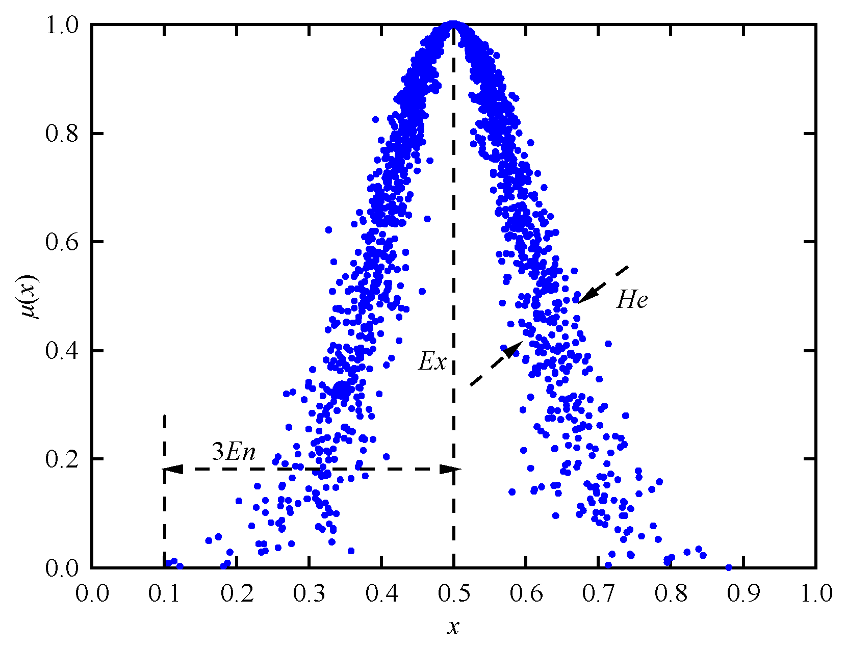
Three numerical characteristics are employed in the cloud model to represent the overall quantitative features of qualitative concepts, namely, expectation (Ex), entropy (En), and hyper entropy (He). Ex is defined as the expected distribution of cloud droplets in the domain space, and is regarded as the point that best represents the qualitative concept; En is used as a measure of the uncertainty of the qualitative concept, and He is used to reflect the degree of dispersion of the cloud droplets [36]. The greater the value of He, the more dispersed the cloud droplets are, and the greater the randomness in the membership degree becomes. As shown in Figure 2, the characteristic values are Ex = 0.5, En = 0.1, and He = 0.02, respectively.

3.4.2. Concept of the Trapezoidal Cloud Model

The normal cloud model uses a single-point expectation (Ex) to represent the core of a qualitative concept, meaning only the value exactly equal to Ex has a certainty degree of 1, while values deviating from Ex see a continuous decline in certainty. However, in practical evaluation processes, describing a certain concept often involves not just a single element fully belonging to that concept, but rather a range of elements within an interval [37]. Therefore, having the expectation as a numerical interval is more general. When the expectation Ex is expressed as a numerical interval, it corresponds to a trapezoidal cloud model [38].

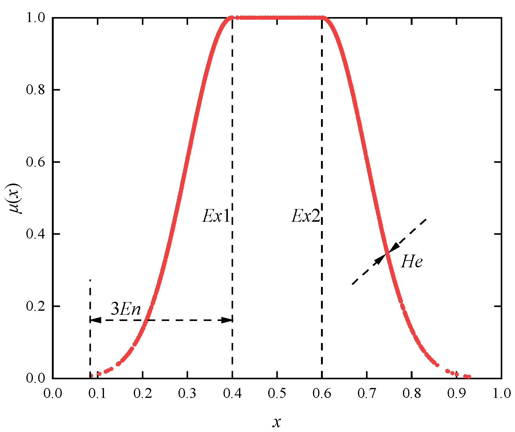
The trapezoidal cloud model is characterized by four numerical cloud features, and the overall quantitative characteristics are expressed using the expectation interval [Ex₁, Ex₂], entropy (En), and hyper entropy (He), as illustrated in Figure 3. The trapezoidal cloud model generalizes the normal cloud by allowing the expectation to be an interval [Ex₁, Ex₂]. Within this core interval, the membership degree remains at 1, which is a more natural and reasonable representation of the qualitative concept that “all values within this range completely belong to this stability level”. This characteristic makes the trapezoidal cloud model particularly suited for simulating the membership relationships in graded evaluation systems like the one in this study. When Ex₁ = Ex₂, the trapezoidal cloud degenerates into a normal cloud [39], indicating that the latter is a special case of the former. The specific calculation steps are as follows:

Step 1: Calculate the numerical characteristics of the trapezoidal cloud model according to Equation (23).

$$\left\{\begin{array}{l}{E}_{x1,ij}={\displaystyle \frac{{\phi }_{ij,\max }+2{\phi }_{ij,\min }}{3}}\\ E_{x2,ij}={\displaystyle \frac{2{\phi }_{ij,\max }+{\phi }_{ij,\min }}{3}}\\ En=({\phi }_{ij,\max }-{\phi }_{ij,\min })/6 \\ He=k\end{array}\right.$$

(23)

where ${\phi }_{ij,\max }$ and ${\phi }_{ij,\min }$ represent the upper and lower limits of the jth evaluation level corresponding to the ith evaluation indicator; k is a constant given based on experience and can be adjusted according to the characteristics of the indicator; in this study, it is set to 0.05.

Step 2: Generate normal random numbers with En as the expectation and He as the standard deviation $E_{nij}^{\prime }$:

$$E_{nij}^{\prime }=randn(1)H_e+E_{nij}$$

(24)

Step 3: Calculate the membership degree μ_ij(x) of the evaluation indicator:

$${\mu }_{ij}(x)=\left\{\begin{array}{cc}\exp (-{(x_i-E_{x1,ij})}^2/2E_{nij}^{\prime })& \hfill x_i<E_{x1,ij}\\ 1\hfill & \hfill E_{x1,ij}\le x_i\le E_{x2,ij}\\ \exp (-{(x_i-E_{x2,ij})}^2/2E_{nij}^{\prime })& \hfill x_i>E_{x2,ij}\end{array}\right.$$

(25)

where μ_ij(x) represents the certainty degree that the value of the ith indicator belongs to the jth level.

Step 4: Determine the evaluation result. Based on the membership degrees calculated by Equation (26), combined with the weights of each evaluation indicator, the comprehensive certainty degree U_i of the evaluated object is calculated as follows:

$$U_i={\displaystyle \sum _{j=1}^n(w_j\times {\mu }_{ij})}$$

(26)

According to the maximum membership principle, the final evaluation level ξ can be obtained as follows:

$$\xi =\max \left\{U_1,U_2,\cdots ,U_i\right\}$$

(27)

4. Results and Discussion

4.1. Results of Comprehensive Variable Weights

(1) Subjective constant weights of evaluation indicators

Based on the theory of the IFAHP, industry experts were invited to perform pairwise comparisons of the nine indicators in the evaluation system using the 0.1~0.9 scale method, and the intuitionistic fuzzy judgment matrix for the evaluation indicator system was constructed. Then, the distance measure was calculated using Equations (2)–(4), resulting in $d(\overline{L},L)=0.0756<0.1$, indicating that L passed the consistency test. The subjective constant weights of each evaluation indicator were then derived using Equations (5)–(7), with the resulting constant weights being 0.1269, 0.1396, 0.1218, 0.1136, 0.0999, 0.0899, 0.0974, 0.1104, and 0.1005, respectively.

$$L=\left[\begin{array}{ccccccccc}(0.5,0.5)& (0.3,0.6)& (0.65,0.25)& (0.55,0.35)& (0.65,0.2)& (0.5,0.45)& (0.35,0.55)& (0.5,0.4)& (0.3,0.6)\\ (0.6,0.3)& (0.5,0.5)& (0.8,0.15)& (0.65,0.25)& (0.9,0.1)& (0.55,0.35)& (0.5,0.45)& (0.6,0.3)& (0.2,0.75)\\ (0.25,0.65)& (0.15,0.8)& (0.5,0.5)& (0.35,0.6)& (0.5,0.45)& (0.2,0.7)& (0.1,0.8)& (0.25,0.65)& (0.25,0.65)\\ (0.35,0.55)& (0.25,0.65)& (0.6,0.35)& (0.5,0.5)& (0.5,0.35)& (0.3,0.6)& (0.2,0.7)& (0.35,0.55)& (0.5,0.4)\\ (0.2,0.65)& (0.1,0.9)& (0.45,0.5)& (0.35,0.5)& (0.5,0.5)& (0.15,0.75)& (0.1,0.85)& (0.2,0.7)& (0.35,0.55)\\ (0.45,0.5)& (0.35,0.55)& (0.7,0.2)& (0.6,0.3)& (0.75,0.15)& (0.5,0.5)& (0.3,0.6)& (0.5,0.45)& (0.5,0.45)\\ (0.55,0.35)& (0.45,0.5)& (0.8,0.1)& (0.7,0.2)& (0.85,0.1)& (0.6,0.3)& (0.5,0.5)& (0.55,0.35)& (0.15,0.8)\\ (0.4,0.5)& (0.3,0.6)& (0.65,0.25)& (0.55,0.35)& (0.7,0.2)& (0.45,0.5)& (0.35,0.55)& (0.5,0.5)& (0.2,0.7)\\ (0.6,0.3)& (0.75,0.2)& (0.65,0.25)& (0.4,0.5)& (0.55,0.35)& (0.45,0.5)& (0.8,0.15)& (0.7,0.2)& (0.5,0.5)\end{array}\right]$$

(2) Objective constant weights of evaluation indicators

In order to enhance the objectivity of the evaluation indicator weights, the improved CRITIC method based on the coefficient of variation was employed, in which both the information volume of indicators and their intercorrelations were comprehensively considered. The coefficient of variation for each indicator was calculated using Equation (9), followed by the calculation of the independence coefficient and importance coefficient of each indicator according to Equations (10) and (11), respectively, and finally, the objective constant weights of the evaluation indicators were obtained based on Equation (12), with the results shown in

Table 3. Objective constant weights of evaluation indicators.

Evaluation Indicators	Coefficient of Variation	Independence Coefficient	Importance Coefficient	Objective Constant Weights
X1	0.1823	9.7717	1.7816	0.0708
X2	0.2403	11.4822	2.7587	0.1097
X3	0.2783	10.9141	3.0369	0.1207
X4	0.2761	8.3687	2.3102	0.0918
X5	0.4373	5.6220	2.4584	0.0977
X6	0.5147	5.8164	2.9939	0.1190
X7	0.5511	5.7524	3.1702	0.1260
X8	0.6062	5.7830	3.5056	0.1393
X9	0.5345	5.8804	3.1428	0.1249

.

(3) Comprehensive constant weights of evaluation indicators

The subjective and objective constant weights were integrated using game theory, and the optimal combination coefficients of subjective and objective constant weights were calculated as 0.4073 and 0.5927, respectively, according to Equations (13)–(18), thereby yielding the integrated constant weights of the evaluation indicators as W* = (0.0936, 0.1219, 0.1211, 0.1007, 0.0986, 0.1071, 0.1144, 0.1275, 0.1151).

(4) Variable weights of evaluation indicators

Based on the theory of variable weights, the evaluation indicator data were initially normalized, followed by constructing the state variable weight vector according to Equation (20), which was then combined with the integrated constant weights to compute the Hadamard product. Ultimately, the variable weights for the evaluation indicators at each stage were calculated using Equation (21), with the outcomes presented in

Table 4. Variable weights of evaluation indicators.

Indicators	Comprehensive Constant Weights	Stage 1	Stage 2	Stage 3
X1	0.0708	0.0939	0.0941	0.0964
X2	0.1097	0.1205	0.1226	0.1264
X3	0.1207	0.1202	0.1206	0.1256
X4	0.0918	0.1010	0.0978	0.1044
X5	0.0977	0.0989	0.0982	0.0983
X6	0.1190	0.1074	0.1077	0.1041
X7	0.1260	0.1147	0.1150	0.1110
X8	0.1393	0.1279	0.1282	0.1224
X9	0.1249	0.1154	0.1157	0.1113

.

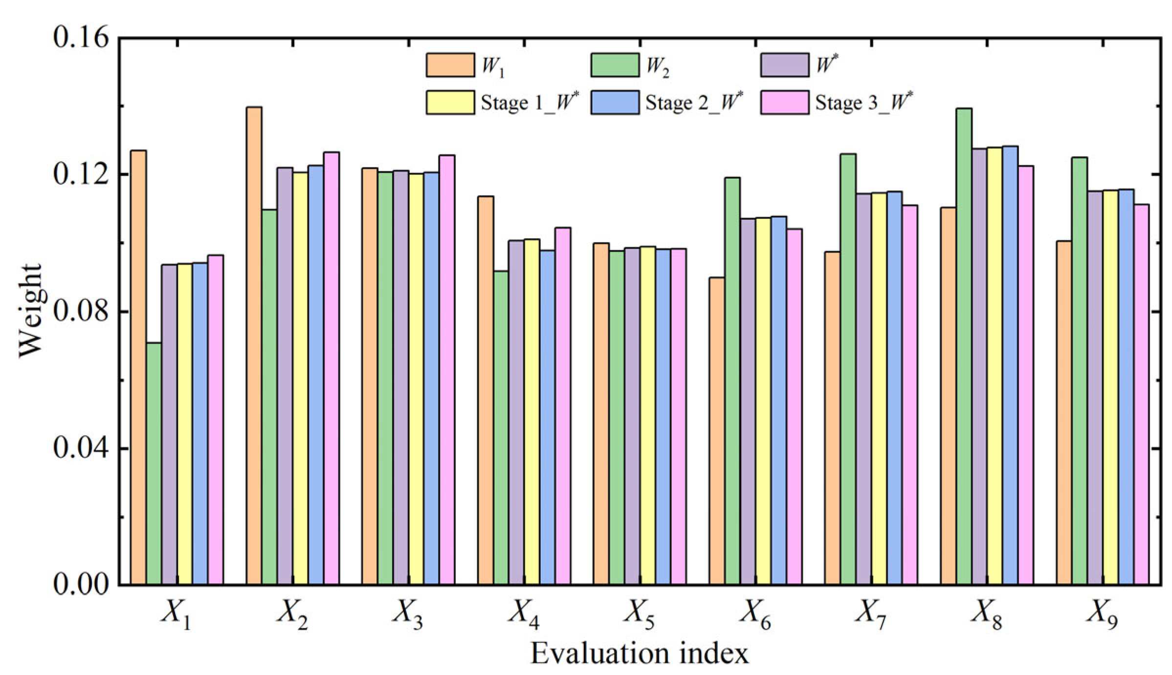
A comparative analysis of the indicator weights calculated by various weighting methods is presented in Figure 4. It can be observed from Figure 4 that the subjective constant weights and objective constant weights of some indicators differ significantly, while the comprehensive constant weights determined by game theory lie between the subjective and objective constant weights, with the overall trend remaining consistent. This reflects that the comprehensive constant weights take into account not only expert subjective judgments but also the intrinsic characteristics of the indicators, thereby rendering the weighting results more scientific and reasonable.

There are certain differences between the dynamic optimal variable weights and the optimal comprehensive constant weights of evaluation indicators at each slope stage, though these differences are not significant. This is because the variable weight theory modifies the comprehensive constant weights based on the state values of each indicator. When the actual values of indicators perform well, the variable weights are less than the constant weights; conversely, when the actual values perform poorly, the variable weights exceed the constant weights, thereby acting as a penalty. That is, the variable weights increase as the indicator values worsen, which to some extent reduces the error caused by constant weights in the evaluation results.

4.2. Evaluation Results Based on the Cloud Model

In order to improve the evaluation of slope stability, the stability of slopes is classified into five grades in this study, with reference to relevant standards and previous research findings on the classification criteria of slope stability or risk assessment indicators. The five grades are defined as: Level I (Highly Stable), Level II (Stable), Level III (Basically Stable), Level IV (Unstable), and Level V (Highly Unstable) [40]. The classification criteria for the value ranges of slope stability evaluation indicators under different grades are presented in

Table 5. Evaluation indicators and grading criteria.

Evaluation Indicator	Stability Level
	I	II	III	IV	V
X1	80~100	60~80	40~60	20~40	0~20
X2	2.1~10	1.5~2.1	0.7~1.5	0.2~0.7	0~0.2
X3	60~90	50~60	39~50	27~39	0~27
X4	0~20	20~40	40~60	60~100	100~150
X5	0~50	50~100	100~150	150~200	200~250
X6	0~20	20~40	40~60	60~80	80~100
X7	0~20	20~40	40~60	60~80	80~100
X8	0~20	20~40	40~60	60~80	80~100
X9	0~20	20~40	40~60	60~80	80~100

.

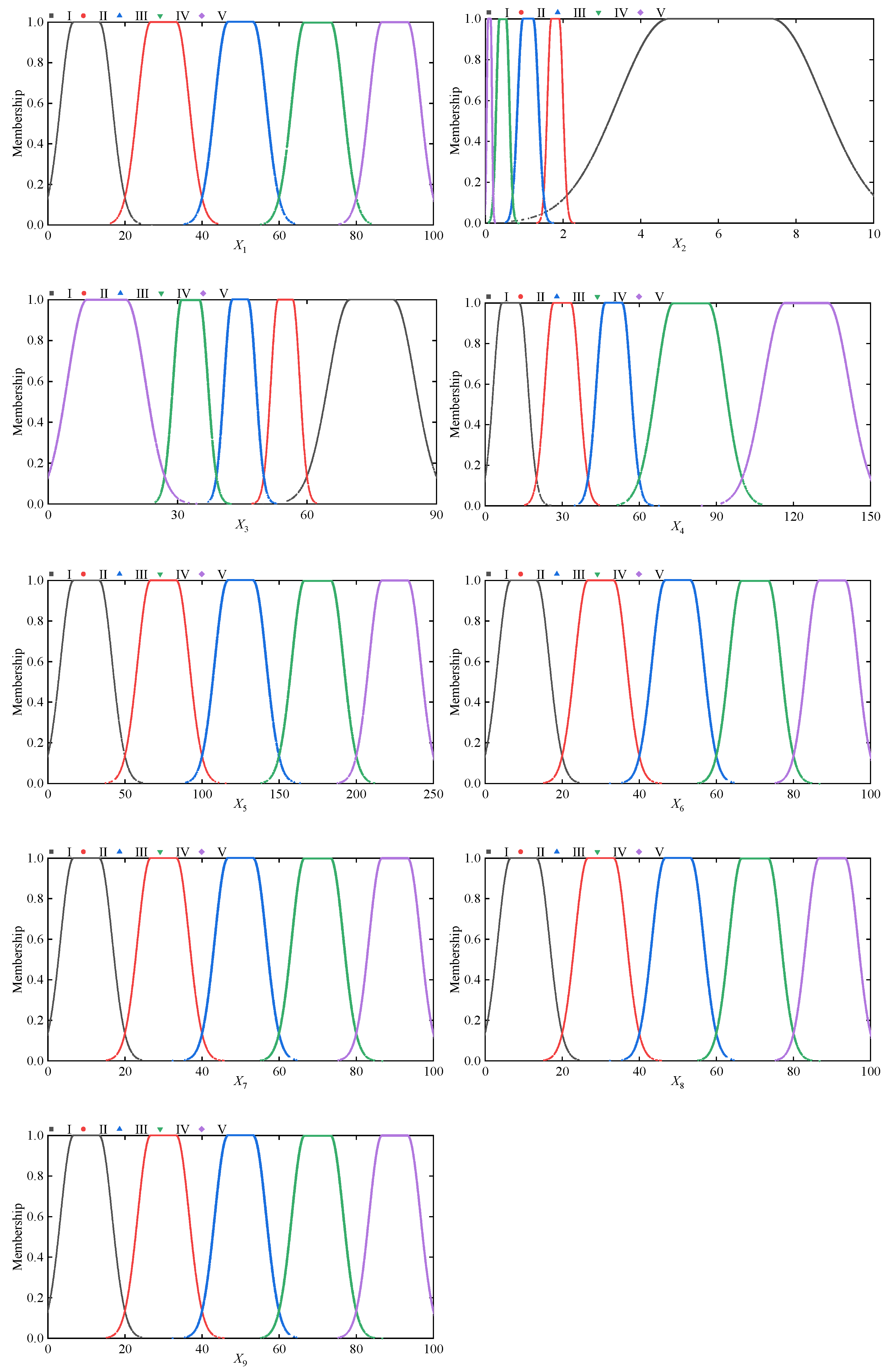
Based on the trapezoidal cloud model theory, the digital characteristics of the trapezoidal cloud model for each evaluation indicator were calculated using Equation (23), as shown in

Table 6. Numerical features of the trapezoidal cloud model for evaluation indicators.

Level	Parameters	X1	X2	X3	X4	X5	X6	X7	X8	X9
I	Ex1	6.67	4.73	70.00	6.67	16.67	6.67	6.67	6.67	6.67
	Ex2	13.33	7.37	80.00	13.33	33.33	13.33	13.33	13.33	13.33
	En	3.33	1.32	5.00	3.33	8.33	3.33	3.33	3.33	3.33
	He	0.05	0.05	0.05	0.05	0.05	0.05	0.05	0.05	0.05
II	Ex1	26.67	1.70	53.33	26.67	66.67	26.67	26.67	26.67	26.67
	Ex2	33.33	1.90	56.67	33.33	83.33	33.33	33.33	33.33	33.33
	En	3.33	0.10	1.67	3.33	8.33	3.33	3.33	3.33	3.33
	He	0.05	0.05	0.05	0.05	0.05	0.05	0.05	0.05	0.05
III	Ex1	46.67	0.97	42.67	46.67	116.67	46.67	46.67	46.67	46.67
	Ex2	53.33	1.23	46.33	53.33	133.33	53.33	53.33	53.33	53.33
	En	3.33	0.13	1.83	3.33	8.33	3.33	3.33	3.33	3.33
	He	0.05	0.05	0.05	0.05	0.05	0.05	0.05	0.05	0.05
IV	Ex1	66.67	0.37	31.00	73.33	166.67	66.67	66.67	66.67	66.67
	Ex2	73.33	0.53	35.00	86.67	183.33	73.33	73.33	73.33	73.33
	En	3.33	0.08	2.00	6.67	8.33	3.33	3.33	3.33	3.33
	He	0.05	0.05	0.05	0.05	0.05	0.05	0.05	0.05	0.05
V	Ex1	86.67	0.07	9.00	116.67	216.67	86.67	86.67	86.67	86.67
	Ex2	93.33	0.13	18.00	133.33	233.33	93.33	93.33	93.33	93.33
	En	3.33	0.03	4.50	8.33	8.33	3.33	3.33	3.33	3.33
	He	0.05	0.05	0.05	0.05	0.05	0.05	0.05	0.05	0.05

. Then, a normal cloud generator program was developed in MATLAB 2021 software, generating trapezoidal cloud model diagrams depicting the affiliation of each indicator to the stability levels, as illustrated in Figure 5.

According to Equation (25), and in combination with the digital characteristics of the trapezoidal cloud model of each evaluation indicator, the certainty degrees of each indicator belonging to the respective stability levels can be calculated. Based on the variable weights of the evaluation indicators, the certainty degrees of each stage’s affiliation to different stability levels were calculated according to Equation (26), and finally, based on the maximum membership principle in Equation (27), the stability level of each stage was determined, as shown in

Table 7. Stability level results at each stage.

Stage	Comprehensive Certainty Degree					Evaluation Grade
	I	II	III	IV	V
Stage 1	0.0602	0.0305	0.4029	0.0493	0.0001	III
Stage 2	0.0934	0.1336	0.1109	0.0731	0.0001	II
Stage 3	0.0984	0.1117	0.0080	0.0788	0.0000	II

. From Table 7, it can be observed that Stage 1 is evaluated as basically stable (III), while both Stage 2 and Stage 3 are assessed as stable (II).

4.3. Numerical Simulation Verification

To verify the accuracy of the evaluation results, numerical simulations were conducted for different stages of the slope. A numerical simulation model was developed using the finite element software FLAC 3D, as illustrated in Figure 6, with a model length of 490 m and a height of 150 m, extending from west to east along the landslide direction. The model consists of 33,006 block elements and 132,024 nodes. The Mohr–Coulomb model was used for soil analysis. Boundary conditions include constraints on horizontal displacements at both sides of the slope, and constraints on both horizontal and vertical displacements at the slope base. Based on the stratigraphy observed in the field, four distinct soil layers were identified. The soil parameters obtained through field measurements and laboratory tests are summarized in

Table 8. Material properties for all parameters used for analyses.

Lithology	Material Properties
	c (kPa)	ϕ (°)	γ (kN/m3)	E (MPa)	μ
Rubble soil	19	25.2	20.1	30	0.26
Pebbles	25	26.1	24.2	28	0.25
Sandstone	26	25.2	23.4	32	0.24
Powdered sandstone	28	26.5	25.4	30	0.26

Note: c, cohesion; ϕ, internal friction angle; γ, unit weight; E, elastic modulus; μ, Poisson’s ratio.

.

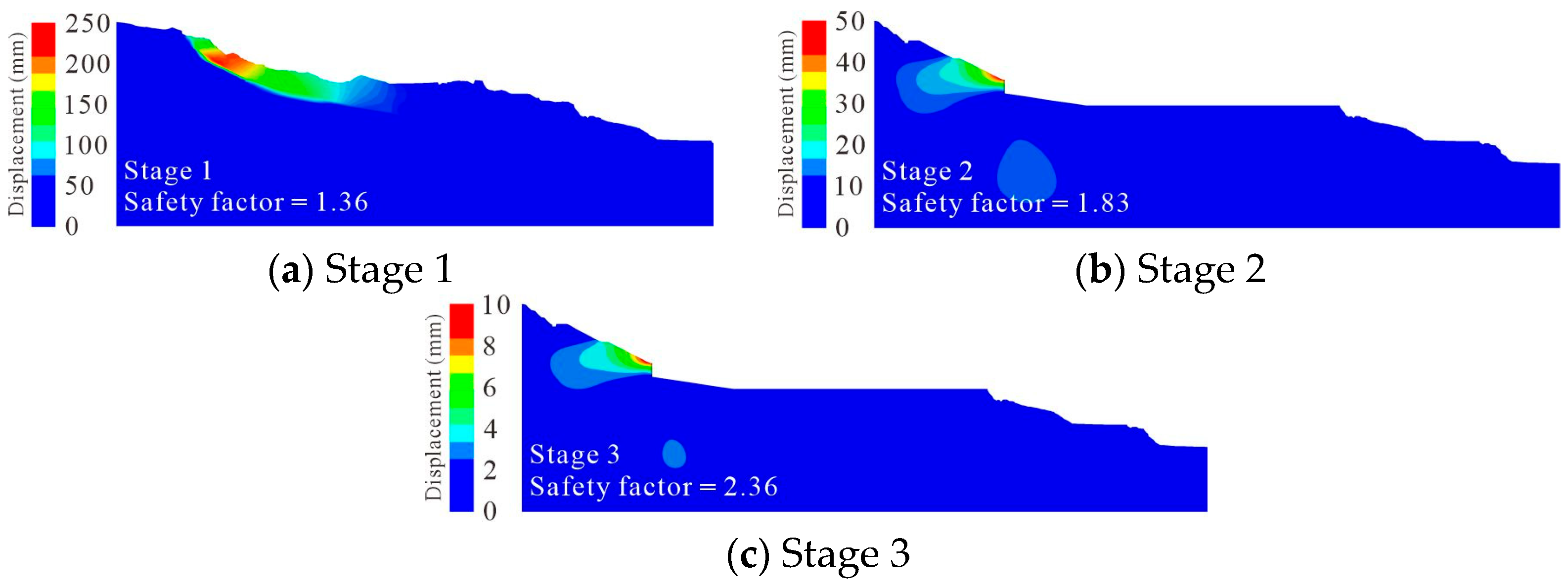
Subsequently, the safety factors for each stage were calculated using the strength reduction method, which involves gradually reducing the cohesion c and internal friction angle φ until slope failure occurs, at which point the reduction coefficient is defined as the slope’s safety factor. Accordingly, the safety factors for Stages 1, 2, and 3 were determined to be 1.36, 1.83, and 2.36, respectively. The displacements corresponding to each stage are illustrated in Figure 7.

Stage 1 (natural condition) yields a slope safety factor of 1.36 based on numerical simulation. Although significant signs of deformation have emerged in the slope body, the shear outlet at the front edge has not yet fully penetrated, indicating that the slope retains a certain degree of stability, and the internal part of the sliding mass still maintains some structural strength. Therefore, it is classified as being in a basically stable condition. Although the slope safety factor has reached a certain level, close attention must still be paid to its potential instability risk. This is consistent with the characteristics of a transitional stage prior to critical failure.

In Stage 2, the combined effects of slope cutting to reduce the sliding mass potential energy and sheet pile wall support to enhance sliding resistance effectively inhibited the development of deformation in the sliding mass. Following preliminary remediation measures applied to the landslide deposit, the safety factor reached 1.83, indicating good stability of the landslide deposit.

In Stage 3, the slope cutting range was further optimized based on previous treatments, with a focus on addressing the middle and lower parts of the sliding mass. After the second round of treatment, the safety factor of the landslide deposit reached 2.36. This indicates that staged unloading significantly improved the stress distribution within the sliding mass, ultimately establishing a multi-level protection system in the remediation works. Therefore, the stability evaluation remains at the stable level, with a further increase in the safety factor.

To further demonstrate the superiority of the proposed model, its evaluation results were compared with those from two widely used methods: the traditional analytic hierarchy process (AHP) and the fuzzy comprehensive evaluation (FCE) method. The same evaluation indicator system and sample data were applied to these two methods for calculation. The comparative results are presented in

Table 9. Comparison of evaluation results from different methods.

Stage	Proposed Model	FCE Method	Traditional AHP	Numerical Simulation
Stage 1	III	II	II	III
Stage 2	II	II	II	II
Stage 3	II	II	II	II

.

As shown in Table 9, for Stage 1, both the traditional AHP and FCE methods evaluated the slope as “Stable (II)”. However, the numerical simulation result (FS = 1.36) and the on-site observations clearly indicate a state of “Basically Stable (III)”, which is accurately captured by the proposed model. This discrepancy arises because the traditional AHP and FCE methods rely on constant weights, which fail to dynamically penalize indicators with poor state values. In contrast, the variable weight theory employed in our model amplifies the weights of these underperforming indicators, leading to a more accurate and conservative assessment that aligns better with the engineering reality. For Stages 2 and 3, all methods concurred with the numerical simulation, as the reinforcement measures improved the overall state of the slope, reducing the penalizing effect of variable weights. This comparison underscores the advantage of the proposed model in enhancing evaluation accuracy, particularly for slopes in a critical or transitional state, by effectively integrating the dynamic impact of indicator states.

This dynamic evaluation process reflects the progressive and targeted nature of the engineering remediation, but attention should be paid to the potential risks associated with deep sliding surfaces, and it is recommended to enhance long-term deformation monitoring. Based on the analysis of the engineering geological characteristics and remediation measures of the three slope stages, it can be concluded that the stability evaluation results are consistent with the numerical simulation outcomes, thereby validating the accuracy of the evaluation results.

5. Conclusions

Slope instability is a common and highly hazardous geological disaster that, once it occurs, poses a severe threat to human lives, property, and various engineering structures, resulting in substantial losses. This study establishes a slope stability evaluation model based on dynamic weighting theory and the trapezoidal cloud model, achieving a dynamic and precise evaluation of slope stability.

(1) Based on the principles of uniqueness, purposefulness, and scientific validity for indicator selection, and drawing on relevant scholarly research, nine evaluation indicators, including rock quality index and internal friction angle, were selected, thereby constructing a slope stability evaluation indicator system, which can objectively and accurately assess the risk levels of slope instability.

(2) The subjective constant weights, objective constant weights, and comprehensive constant weights of the evaluation indicators were determined, respectively by using IFAHP, an enhanced CRITIC method, and game theory approach, followed by dynamic modification of the integrated constant weights according to the dynamic weighting theory, effectively addressing the imbalance of weights resulting from the dynamic changes in the evaluation indicators.

(3) A trapezoidal cloud model combined with variable weights of evaluation indicators was employed to develop a dynamic stability assessment model for slopes, effectively addressing the uncertainty and randomness inherent in the risk assessment process. The model was applied to the engineering case study, and the results indicated that the slope stability at Stage 1 was classified as basically stable, while the stability levels at Stages 2 and 3 were classified as stable, and the evaluation model’s accuracy was validated through numerical simulation. The research findings offer novel approaches and valuable references for slope stability risk assessment.

References

1. Kumar, P.R.; Muthukkumaran, K.; Sharma, C. Technological advancements and sustainable practices in rock slope stability–Critical review. Phys. Chem. Earth 2024, 136, 103699. [Google Scholar] [CrossRef]
2. Zhang, X.; Li, Z.; Wei, S.; Li, D.; Li, X.; Xin, R.; Hu, W.; Liu, H.; Guan, P. Study on the Distribution Characteristics of Thermal Melt Geological Hazards in Qinghai Based on Remote Sensing Interpretation Method. Water 2025, 17, 2295. [Google Scholar] [CrossRef]
3. Wang, G.; Zhao, B.; Wu, B.; Zhang, C.; Liu, W. Intelligent prediction of slope stability based on visual exploratory data analysis of 77 in situ cases. Int. J. Min. Sci. Technol. 2023, 33, 47–59. [Google Scholar] [CrossRef]
4. Zhang, W.G.; Li, H.R.; Han, L.; Chen, L.L.; Wang, L. Slope stability prediction using ensemble learning techniques: A case study in Yunyang County, Chongqing, China. J. Rock Mech. Geotech. 2022, 14, 1089–1099. [Google Scholar] [CrossRef]
5. Moayedi, H.; Osouli, A.; Nguyen, H.; Rashid, A.S.A. A novel Harris hawks’ optimization and k-fold cross-validation predicting slope stability. Eng. Comput. 2021, 37, 369–379. [Google Scholar] [CrossRef]
6. Nguyen, P.M.V.; Wrana, A.; Rajwa, S.; Różański, Z.; Frączek, R. Slope stability numerical analysis and landslide prevention of coal mine waste dump under the impact of rainfall—A case study of Janina Mine, Poland. Energies 2022, 15, 8311. [Google Scholar] [CrossRef]
7. Chand, K.; Koner, R. Failure zone identification and slope stability analysis of mine dump based on realistic 3D numerical modeling. Geotech. Geol. Eng. 2024, 42, 543–560. [Google Scholar] [CrossRef]
8. Kumar, A.; Roy, L.B. Analysis of Slope Failure in Ostapal Open Pit Chromite Mine Using Numerical Modelling in FLAC—A Case Study. Indian Geotech. J. 2025, 1–12. [Google Scholar] [CrossRef]
9. Pei, T.; Qiu, T.; Shen, C.P. Applying knowledge-guided machine learning to slope stability prediction. J. Geotech. Geoenviron. 2023, 149, 04023089. [Google Scholar] [CrossRef]
10. Huang, F.M.; Xiong, H.W.; Chen, S.X.; Lv, Z.Y.; Huang, J.S.; Chang, Z.L.; Catani, F. Slope stability prediction based on a long short-term memory neural network: Comparisons with convolutional neural networks, support vector machines and random forest models. Int. J. Coal Sci. Technol. 2023, 10, 18. [Google Scholar] [CrossRef]
11. Sabri, M.S.; Ahmad, F.; Samui, P. Slope stability analysis of heavy-haul freight corridor using novel machine learning approach. Model. Earth Syst. Environ. 2024, 10, 201–219. [Google Scholar] [CrossRef]
12. Chen, Z.Y.; Dai, Z.H. Application of group decision-making AHP of confidence index and cloud model for rock slope stability evaluation. Comput. Geosci. 2021, 155, 104836. [Google Scholar] [CrossRef]
13. Bai, M.Z.; Yang, L.; Liu, L.X.; Long, W.X.; Xiang, Y.M. Risk assessment of gently inclined mudstone bedding slope incorporating monitoring information. Geomat. Nat. Hazards Risk 2025, 16, 2452349. [Google Scholar] [CrossRef]
14. Wu, G.; Nie, X.; Zhang, X.; Yang, M.; Shi, G. Stability Grade Evaluation of Slope with Soft Rock Formation in Open-Pit Mine Based on Modified Cloud Model. Sustainability 2024, 16, 4706. [Google Scholar] [CrossRef]
15. Yang, X.; Hao, Z.; Ma, G.; Li, G. Research on Slope Stability Evaluation Based on Improved Set Pair Analysis Method: A Case of Tonglvshan Open-Pit Mine. Shock. Vib. 2021, 2021, 6713581. [Google Scholar] [CrossRef]
16. Deng, D. Limit equilibrium solution for the rock slope stability under the coupling effect of the shear dilatancy and strain softening. Int. J. Rock Mech. Min. 2020, 134, 104421. [Google Scholar] [CrossRef]
17. Liu, L.L.; Dou, Y.M.; Qiao, J.G. Evaluation method of highway plant slope based on rough set theory and analytic hierarchy process: A case study in Taihang Mountain, Hebei, China. Mathematics 2022, 10, 1264. [Google Scholar] [CrossRef]
18. Wang, J.; Hu, B.; Li, J.; Chang, J.; Cui, A.N.; Cui, K. Evaluation method of mine slope stability based on unascertained measure theory. Chin. J. Nonferr. Met. 2021, 31, 1388–1394. (In Chinese) [Google Scholar]
19. Yang, Y.; Yang, Z.; Xu, W.; A, F.; Guo, Y.; Zheng, J. Research on the Failure Mechanism and Treatment Technology of Landslides in Typical Accumulation Bodies Along Highways in Qinghai Province. Water 2025, 17, 34. [Google Scholar] [CrossRef]
20. Yu, X.; Zheng, D.; Zhou, L. Credit risk analysis of electricity retailers based on cloud model and intuitionistic fuzzy analytic hierarchy process. Int. J. Energy Res. 2021, 45, 4285–4302. [Google Scholar] [CrossRef]
21. Wang, J.; Liu, S.; Song, Y.; Wang, J.; Wu, H. Environmental risk assessment of subway station construction to achieve sustainability using the intuitionistic fuzzy analytic hierarchy process and set pair analysis. Discret. Dyn. Nat. Soc. 2021, 2021, 5541493. [Google Scholar] [CrossRef]
22. Song, Q.; Xue, Y.; Li, G.; Su, M. Using Bayesian network and Intuitionistic fuzzy Analytic Hierarchy Process to assess the risk of water inrush from fault in subsea tunnel. Geomech. Eng. 2021, 27, 605–614. [Google Scholar] [CrossRef]
23. Chen, Y.L.; Shen, S.L.; Zhou, A. Assessment of red tide risk by integrating CRITIC weight method, TOPSIS-ASSETS method, and Monte Carlo simulation. Environ. Pollut. 2022, 314, 120254. [Google Scholar] [CrossRef] [PubMed]
24. Krishnan, A.R.; Kasim, M.M.; Hamid, R.; Ghazali, M.F. A modified CRITIC method to estimate the objective weights of decision criteria. Symmetry 2021, 13, 973. [Google Scholar] [CrossRef]
25. Peng, J.; Zhang, J. Urban flooding risk assessment based on GIS-game theory combination weight: A case study of Zhengzhou City. Int. J. Disaster Risk Reduct. 2022, 77, 103080. [Google Scholar] [CrossRef]
26. He, X.; Gao, C.; Cao, H.Z.; Li, Y.; Yu, T. Evaluation of distribution network index based on improved analytic hierarchy process. Electr. Meas. Instrum. 2022, 59, 93–99. (In Chinese) [Google Scholar]
27. Xiang, S.Y.; Cai, Z.X.; Liu, P.; Li, L.N. Fuzzy comprehensive evaluation of low carbon operation of distribution network based on AHP-inverse entropy weight method. J. Electr. Power Sci. Technol. 2019, 34, 69–76. (In Chinese) [Google Scholar]
28. Li, N.; Fan, Z.F.; Liu, X. Impact evaluation of prefabricated buildings cost on game theory-cloud model. J. Math. 2022, 2022, 3635009. [Google Scholar] [CrossRef]
29. Han, F.; Liu, Z.; Wang, C. Research on a comfort evaluation model for high-speed trains based on variable weight theory. Appl. Sci. 2023, 13, 3144. [Google Scholar] [CrossRef]
30. Zhang, G.D.; Xue, Y.G.; Bai, C.H.; Su, M.X.; Zhang, K.; Tao, Y.F. Risk assessment of floor water inrush in coal mines based on MFIM-TOPSIS variable weight model. J. Cent. South Univ. 2021, 28, 2360–2374. [Google Scholar] [CrossRef]
31. Yao, B.; Wang, L.; Gao, H.; Ren, L. Bridge construction risk assessment based on variable weight theory and cloud model. Buildings 2024, 14, 576. [Google Scholar] [CrossRef]
32. Guo, D.S.; Meng, F.Y.; Wu, H.N.; Yang, X.X.; Liu, Z. Risk assessment of shield tunneling crossing building based on variable weight theory and cloud model. Tunn. Undergr. Space Technol. 2024, 145, 105593. [Google Scholar] [CrossRef]
33. Wang, L.; Guo, Q.; Luo, J.; Zhang, Y.; Wan, Z.; Wang, X. A novel evaluation method for the stability of construction sites on an abandoned goaf: A case study. KSCE J. Civ. Eng. 2022, 26, 2835–2845. [Google Scholar] [CrossRef]
34. Chen, H.; Shen, Q.; Feng, Z.; Liu, Y. Vulnerability assessment in urban metro systems based on an improved cloud model and a Bayesian network. KSCE J. Civ. Eng. 2023, 98, 104823. [Google Scholar] [CrossRef]
35. Jiao, L.; Zhu, Y.; Huo, X.; Wu, Y.; Zhang, Y. Resilience assessment of metro stations against rainstorm disaster based on cloud model: A case study in Chongqing, China. Nat. Hazards 2023, 116, 2311–2337. [Google Scholar] [CrossRef] [PubMed]
36. Bai, M.; Liu, Q. Evaluating urban fire risk based on entropy-cloud model method considering urban safety resilience. Fire 2023, 6, 62. [Google Scholar] [CrossRef]
37. Lu, Y.; Fang, G.; Deng, M.; Fang, G.; Zhu, Z.; Sun, C.; Yang, Z. Ecological health assessment of riparian zone of Yangtze River based on trapezoid cloud model in Jiangsu Province, China. Ecol. Indic. 2024, 169, 112796. [Google Scholar] [CrossRef]
38. Feng, Z.; Zhou, X.; Dong, J.; Chen, H.; Liu, Y. Advancing Public–Private Partnerships in Waste Management Facilities: A Risk Assessment Framework based on a trapezoidal cloud model and Bayesian network. Appl. Soft Comput. 2025, 182, 113565. [Google Scholar] [CrossRef]
39. Yang, Z.; Huang, X.; Fang, G.; Ye, J.; Lu, C. Benefit evaluation of East Route Project of South to North Water Transfer based on trapezoid cloud model. Agric. Water Manag. 2021, 254, 106960. [Google Scholar] [CrossRef]
40. Zhao, X.R.; Li, Y.F.; Gao, S.; Chen, K.L. Stability evaluation method of railway rock slope based on combinatorial weight-set pair analysis. Railw. Constr. 2021, 61, 93–97. (In Chinese) [Google Scholar]
Figure 1. Geographic location of the study area: (a) location in Qinghai Province; (b) panoramic image of the landslide; (c) landslide geological profile diagram.
Water 17 03016 g001
Figure 2. Schematic of the normal cloud model.
Water 17 03016 g002
Figure 3. Schematic of the trapezoidal cloud model.
Water 17 03016 g003
Figure 4. Comparison of weights by different weighting methods (W1: subjective constant weight; W2: objective constant weight; W*: comprehensive constant weight; Stage 1_W*: Stage 1 comprehensive constant weight; Stage 2_W*: Stage 2 comprehensive constant weight; Stage 3_W*: Stage 3 comprehensive constant weight).
Water 17 03016 g004
Figure 5. Trapezoidal cloud model of evaluation indicators.
Water 17 03016 g005
Figure 6. Numerical simulation model diagram.
Water 17 03016 g006
Figure 7. The results of numerical simulations at different stages.
Water 17 03016 g007