Article

Quantifying Flood Impacts on Ecosystem Carbon Dynamics Using Remote Sensing and Machine Learning in the Climate-Stressed Landscape of Emilia-Romagna

Department of Civil, Environmental and Architectural Engineering (DICEA), University of Padova, Via Ognissanti, 39, 35131 Padova, Italy
*
Authors to whom correspondence should be addressed.
Water 2025, 17(20), 3001; https://doi.org/10.3390/w17203001 (registering DOI)
Submission received: 25 July 2025 / Revised: 10 October 2025 / Accepted: 13 October 2025 / Published: 18 October 2025

Abstract

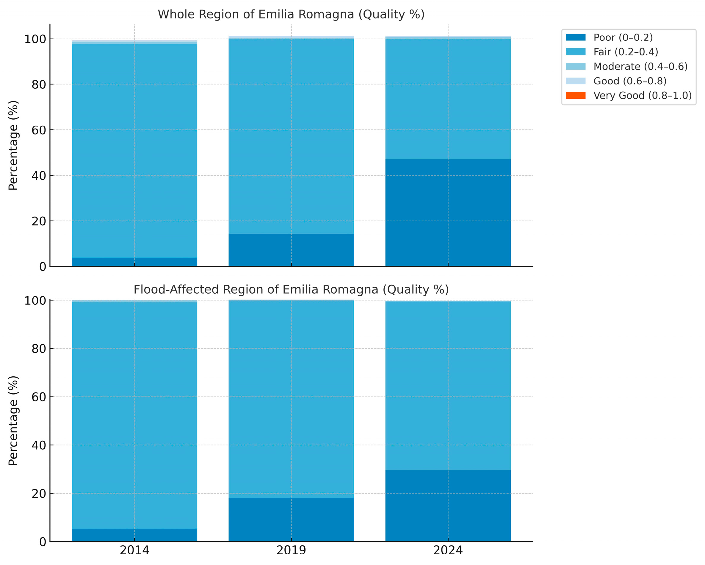
Flood events, intensified by climate change, pose significant threats to both human settlements and ecological systems. This study presents an integrated approach to evaluate flood impacts on ecosystem carbon dynamics using remote sensing and machine learning techniques. The case of the Emilia-Romagna region in Italy is presented, which experienced intense flooding in 2023. To understand flood-induced changes in the short term, we quantified the differences in net primary productivity (NPP) and above-ground biomass (AGB) before and after flood events. Short-term analysis of NPP and AGB revealed substantial localized losses within flood-affected areas. NPP showed a net deficit of 7.0 × 10³ g C yr−1, and AGB a net deficit of 0.5 × 10³ Mg C. While the wider region gained NPP (6.7 × 10⁵ g C yr−1), it suffered a major AGB loss (3.3 × 10⁵ Mg C), indicating widespread biomass decline beyond the flood zone. Long-term ecological assessment using the Remote Sensing Ecological Index (RSEI) showed accelerating degradation, with the “Fair” ecological class shrinking from 90% in 2014 to just over 50% in 2024, and the “Poor” class expanding. “Good” and “Very Good” classes nearly disappeared after 2019. High-hazard flood zones were found to contain 9.0 × 10⁶ Mg C in AGB and 1.1 × 10⁷ Mg C in soil organic carbon, highlighting the vulnerability of carbon stocks. This study underscores the importance of integrating flood modeling with ecosystem monitoring to inform climate-adaptive land management and carbon conservation strategies. It represents a clear, quantifiable carbon loss that should be factored into regional carbon budgets and post-flood ecosystem assessments.

1. Introduction

Flooding is among the most frequent and damaging natural disasters worldwide [1], causing substantial losses to human lives, infrastructure, and ecosystems [2,3]. Driven by the intensifying hydrological cycle under climate change, flood events are becoming increasingly erratic and severe [4,5], often resulting in extensive ecological disruptions. As per the Intergovernmental Panel on Climate Change (IPCC) [6], flooding is one of the key climate-related risks facing both urban and rural regions [7]. In Europe, evidence indicates that extreme precipitation events have surged in both magnitude and intensity since the 1950s [8]. Extreme rainfall is emerging as a primary trigger for river floods [9]. However, flood dynamics are complex and influenced by a number of factors. For instance, stream morphology [10] and interventions in river and catchment engineering [11] play critical roles, while evolving land-use and land-cover patterns [12,13] further modulate flood behavior. Additionally, intricate feedback among climate, soil, snow, and vegetation [14,15] contributes to the flooding event. Although extensive research has focused on the vulnerabilities of human settlements and infrastructure to flooding, the implications for ecosystem function, specifically vegetation productivity and carbon cycle, remain comparatively underexplored. These aspects merit further rigorous study to fully understand the environmental consequences of an increasingly flood-prone climate.
Vegetated ecosystems such as forests [16], wetlands, and grasslands [17,18] serve as crucial carbon sinks by sequestering carbon through photosynthesis and storing it in biomass and soils. Flood events can drastically alter these processes, either temporarily disrupting plant productivity or permanently transforming the structure and function of landscapes [19]. These disturbances can result in the loss of above-ground biomass (AGB), reductions in net primary productivity (NPP), shifts in soil organic carbon (SOC) dynamics due to erosion, inundation, or changes in microbial activity, leading to a general reduction in ecological quality.
Understanding the relationship between flood hazards and ecosystem carbon storage is essential for developing integrated disaster risk reduction and climate adaptation strategies. Recent advances in spatial flood susceptibility modeling using artificial intelligence have enhanced our ability to identify and interpret high-risk flood zones, thereby informing risk-sensitive ecological planning [20]. At the same time, ecosystem-based adaptation approaches such as wetland restoration and green infrastructure have proven effective in mitigating multi-hazard risks while simultaneously preserving or enhancing carbon storage, particularly in ecologically sensitive and delta regions [21]. However, assessing such interactions at landscape scales remains a challenge due to the need for spatially detailed, temporally consistent, and ecologically relevant data.
Recent advances in remote sensing and cloud computing platforms such as Google Earth Engine (GEE) have revolutionized the way environmental changes are monitored and analyzed [22]. These tools enable near real-time access to vast archives of satellite data, allowing researchers to track land surface dynamics with high spatial and temporal resolution [23]. Recent developments in spaceborne lidar and altimetry have demonstrated growing potential for hydrological and flood applications that are complementary to multispectral and SAR approaches. Several studies have shown that ICESat-2 altimetry can provide precise water-level measurements for inland water bodies and reservoirs [24], improving the delineation of inundation dynamics during flood events and providing direct hydrological constraints for impact assessments [25]. Research has also demonstrated that ICESat-2 elevation and water-height measurements can be used to infer river cross-sectional shapes and support hydraulic modeling, which in turn enhances flood extent and depth estimation [26]. At the ecosystem level, studies combining SAR, lidar, and optical data have successfully mapped aboveground carbon in flood-exposed forests and quantified biomass vulnerability to inundation [27]. Recent applications to the Emilia-Romagna floods further illustrate how satellite-based inundation mapping and flood-hazard models can be combined with ecosystem assessments to evaluate environmental impacts at a regional scale [28,29]. Integrating flood- and water-level products with optical- and SAR-derived ecosystem metrics (AGB, NPP, RSEI) therefore offers a promising pathway to better quantify carbon stocks at risk from flooding and to improve temporal characterization of flood pulses that drive rapid carbon exchange.
RSEI has been widely applied to monitor ecological quality and environmental change across different regions [23]. Case study shows sharp declines in RSEI after large disturbance events [30,31], demonstrating RSEI’s ability to capture medium- to short-term ecological degradation and gradual recovery trajectories. Recent extreme events, such as the May 2023 Emilia-Romagna floods and landslides [32], highlight the urgent need to assess how such hazards directly influence ecological conditions.
Remote sensing-derived metrics like AGB, NPP, and RSEI can be used to assess pre- and post-flood vegetation dynamics, providing insights into carbon fluxes and recovery trajectories across the landscape (see Table 1). Understanding how floods affect carbon storage and ecosystem productivity is critical for developing resilient land management and conservation strategies in flood-prone regions [33]. At present, the impact mechanism of the flooding on ecological quality is not explored fully.
This study aims to bridge the gap between flood events and ecosystem responses through a remote sensing-based approach. The objectives are threefold. First, to evaluate the impact of flooding at short term, by analyzing changes in NPP and carbon stocks in terms of AGB between the pre- and flood-event period. Short-term changes in SOC cannot be analyzed in this study because temporally consistent SOC data are not available. Second, to assess the dynamics of ecosystem health over the last decade by examining changes in RSEI. Third, to estimate the carbon stocks, in terms of SOC and AGB, that are vulnerable to high-risk flood-hazard zones.
By integrating flood-hazard data, satellite-derived vegetation indices, and machine learning techniques, this study aims to provide a comprehensive understanding of the interplay between flooding events and ecosystem carbon dynamics, ultimately informing climate-adaptive land management and carbon conservation strategies.
This study considers the Emilia-Romagna region in Italy, which experienced two severe flooding events within two weeks (2–3 May and 15–17 May 2023), characterized by the simultaneous overflow of 23 rivers, releasing an estimated volume of approximately 350 million cubic meters of floodwater. Additionally, the event triggered a widespread geomorphological crisis, with 65,598 landslides, including rapid earth and debris slides, mudflows, and rockslides, recorded across an area of 72.21 km2 [34]. For medium-term analysis of ecosystem carbon dynamics during the period of 2014–2024 in the Emilia-Romagna region and the flood-affected region, three flooding events were witnessed within this period.
The novelty of this study lies in its integrated framework that combines flooding with ecological impact assessment using cloud-based geospatial analysis. By using open-access satellite data and scalable tools in GEE, the approach is both replicable and adaptable to other regions facing similar flood risks. Furthermore, linking flood dynamics to carbon storage adds a valuable ecosystem services dimension to flood risk analysis, offering insights relevant for both disaster risk reduction and climate change mitigation efforts.
The current results serve as an early step towards a deeper understanding of flood impacts. The analyses based on satellite data provide initial observations without fully capturing the complexity of flood dynamics and ecosystem responses, and they should be integrated with field data and longer time series.

2. Materials and Methods

This study employs a multi-source, cloud-based remote sensing workflow in GEE to quantify the short-term impacts of the May 2023 flood event and the decadal changes from 2014 to 2024 on ecosystem carbon dynamics in the Emilia-Romagna region (Italy) and the flood-affected area. In addition, the carbon stocks, in terms of SOC and AGB, stored in highly susceptible flood zones are evaluated. Figure 1 represents a flow chart of the workflow, Table 2 summarizes the objectives and indicators used, and Table 3 reports the databases used for the analyses.
The May 2023 flood extent was delineated from Copernicus EMS (EMSN154) to define the flood-affected region. The boundary of the Emilia-Romagna region coincides with the administrative boundary, and the metrics evaluated in this area are named “whole Emilia-Romagna”.
Indicators that are used as a reference for the year considered and available with more frequent time resolution are calculated as averages over the period.
In order to evaluate the short-term impact of flooding, net primary productivity and above-ground biomass density (AGBD) are used. A TVDI-based water stress coefficient approach using Carnegie–Ames–Stanford Approach (CASA) model was employed to calculate annual NPP for year 2022 (pre-event) and 2023 (event-year), as better explained in Section 2.1. AGBD was retrieved from NASA’s GEDI mission and elaborated as explained in Section 2.2. Subsequently, the flood-induced changes in AGB and NPP were evaluated by calculating the difference between the pre-event and event-year estimates. The spatial extent of the areas that showed an increase or a decrease in AGB or NPP, and the total variation over the area of interest, were calculated.
The procedure to assess long-term ecological changes from 2014 to 2024 uses RSEI and is explained in detail in Section 2.3.
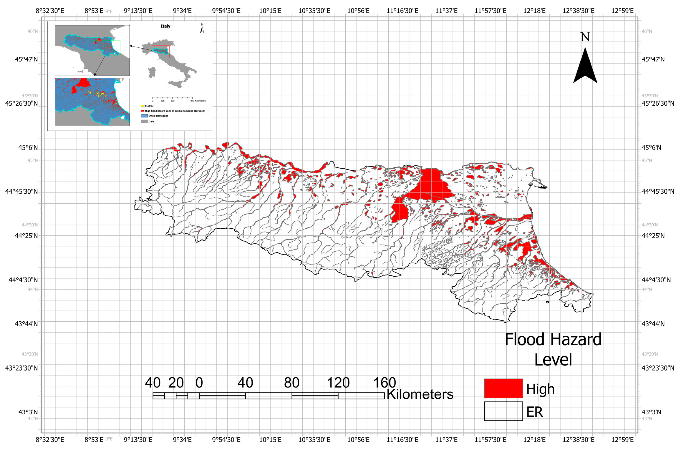
Finally, high flood-hazard zones identified by the Idrogeo [35] dataset were integrated and overlaid with the SOC and AGB layers. Within these masked high-hazard polygons, the total SOC and AGB stocks were summed up to reveal the distribution of carbon stocks within flood-risk areas and quantify the carbon stocks potentially at risk from flooding. This analysis aimed to understand the amount of SOC and AGB stored in areas with high flood risk.
All data processing, modeling, map generation, and exports were executed within GEE’s Code Editor, and final finishing of the map was performed using ARCGIS Pro, ensuring a reproducible, spatially explicit framework for integrated disaster risk and carbon-cycle analysis.
Table 2. Tabular representation of the objectives, indicators, and databases adopted.
ObjectiveIndicators UsedDatabases Used
Short-Term Analysis (Pre- and Post-event) AGB and NPP[36,37]
Medium-Term Analysis (10 years)RSEI[38]
Calculation of Total Carbon for High-Hazard LevelAGB and SOC[36,39]
Table 3. Data utilized in the study.
DataResolutionSourceURL
NDVI30 mGoogle Earth Enginehttps://developers.google.com/earth-engine/datasets/catalog/landsat-8 (accessed on 15 May 2025)
DEM30 mGoogle Earth Enginehttps://developers.google.com/earth-engine/datasets/catalog/COPERNICUS_DEM_GLO30#Earth Engine Data Catalog|Google for Developers (accessed on 27 April 2025).
SOC100 mRegione Emilia-Romagna Ambiente and accessed through minERva Portal(Application Maps—Organic carbon stored in regional soils between 0 and 30 cm—third edition—Dataset—minERva (accessed on 5 April 2025)
NPP/GPP30 mGoogle Earth Enginehttps://developers.google.com/earth-engine/datasets/catalog/LANDSAT_LC08_C02_T1_L2
Earth Engine Data Catalog|Google for Developers (accessed on 15 May 2025)
AGBD25 mGoogle Earth EngineRasterization: Google and USFS Laboratory for Applications of Remote Sensing in Ecology (LARSE) NASA GEDI mission, accessed through the USGS LP DAAC
Flood Polygons-CopernicusEMSN154|Copernicus EMS on Demand Mapping)
RSEI30Google Earth EngineLandsat Collection 2 Level 2 Science Products|U.S. Geological Survey
High Flood-Hazard Zones-IdroGEO—ISPRAIdroGEO—Hazard and Risk

2.1. Changes in NPP in Flooded Areas

To evaluate temporal changes in NPP following flood events, annual NPP was assessed over the Emilia-Romagna region of Italy for the years 2022 and 2023 using remote sensing data in combination with an ecosystem productivity model. The methodology was adapted from an open-source script originally developed by Luana Becker da Luz (2025) [40] and subsequently modified for the purposes of this study (for details see Appendix A). Implementation was conducted on the GEE platform using data available on GEE, which enables scalable, cloud-based geospatial analysis.
NPP values were expressed in grams of carbon per square meter per year (g C m−2 yr−1). The resulting annual NPP maps were spatially clipped to the Emilia-Romagna region and to flood-affected polygons, then exported at 30 m resolution. These outputs were subsequently imported into ArcGIS Pro for visualization and map production.
The difference in annual NPP obtained at pixel level between the 2022 (pre-event) and 2023 (event) was calculated and used to compute extensions of areas that experienced increases or decreases in this indicator. Total annual NPP was estimated by multiplying the NPP value by the area at pixel level and summing across the study area. The difference in total annual NPP between the two years, 2022 (pre-event) and 2023 (event), was used to assess the flood impact on the productivity of the ecosystem.

2.2. Changes in Above-Ground Biomass Density (AGBD) in Flooded Areas

To analyze the impact of floods on carbon stocks in the area affected by the May 2023 event, we implemented a multi-source remote sensing approach using GEE to quantify the changes in AGB. NASA’s GEDI mission data, providing LIDAR-based AGB density (AGBD) at 25 m resolution, were used as a reference (for details, see Appendix A). Quality-filtered GEDI points were combined with Sentinel-2 spectral bands, vegetation indices, and topographic variables (elevation and slope) to train a regression model for predicting AGBD. Sentinel-2 imagery was cloud-masked and composited annually. The trained model was applied to estimate spatially continuous AGBD across the flood polygons. Non-vegetated pixels were excluded using ESA World Cover.
Differences in AGBD at the pixel level were used to compute the extent of areas that experienced an increase or decrease in this indicator. Total annual AGB was computed by multiplying the density by the area at the pixel level and summing across the study area. The difference in total annual AGB between the two years, 2022 (pre-event) and 2023 (event), was used to assess flood-induced carbon stock loss.

2.3. Changes in RSEI (Remote Sensing Ecological Index) over a Decade

To obtain the RSEI, we employed a multiphase workflow approach based on Yan et al., 2021 [41], for assessing environmental conditions and their temporal changes using remote sensing data on GEE (for details see Appendix A). Firstly, Landsat 8 Surface Reflectance imagery was processed for the years 2014, 2019, and 2024, with cloud and shadow masking applied. Four environmental indicators are derived: NDVI (vegetation greenness), Tasseled Cap Wetness (moisture), NDBSI (built-up index), and LST (land surface temperature). These indicators were normalized to a 0–1 scale and exported for further analysis. RSEI was divided into five classes, namely Poor (0–0.2), Fair (0.2–0.4), Moderate (0.4–0.6), Good (0.6–0.8), and Very Good (0.8–1.0), to analyze spatial and temporal changes between the years 2014, 2019, and 2024, and to further analyze the transition between 2014 and 2024 among the different classes (adapted from Yan et al. [41]). The change levels are defined as S + 4, S + 3, S + 2, S + 1, S 0, S–1, S–2, S–3, and S–4. S denotes state and Levels +4, +3, +2, and +1 correspond to ecological improvements of degrees 4 through 1, respectively. Level S0 indicates no change/stable ecological conditions, while levels −1, −2, −3, and −4 denote successive degrees of degradation. Area changes were computed for the Emilia-Romagna area (whole region) and the flood-affected region and exported as summary tables for interpretation. The whole process was completely performed on the GEE platform.

2.4. SOC and AGB Within Flood-Hazard Categories

The map of SOC for year 2023 was taken from Regione Emilia-Romagna Ambiente and accessed through the minERva Portal [42] for the Emilia-Romagna region, which provides the data on the organic carbon content in Mg/ha in the first 30 cm of soil at a resolution of 100 m (for details, see Appendix A). The workflow began by importing the region of interest (high-flood region polygons) as an Earth Engine Feature Collection of polygons and loading the SOC raster, whose pixel values represent carbon density in Mg per hectare. We then converted those per hectare values into total Mg per pixel by multiplying each pixel’s value by its area in hectares. Next, for each polygon we computed its area (in m2) and ran a reduce region with a sum reducer over the converted SOC image, which yielded the total Mg of carbon contained within that individual polygon. Finally, we obtained the grand total by aggregating the per-polygon sums via aggregate sum of SOC stock (in Mg), strictly confined to the region of interest. Similar steps were adopted to calculate AGB, and the whole process was performed on GEE.

3. Results

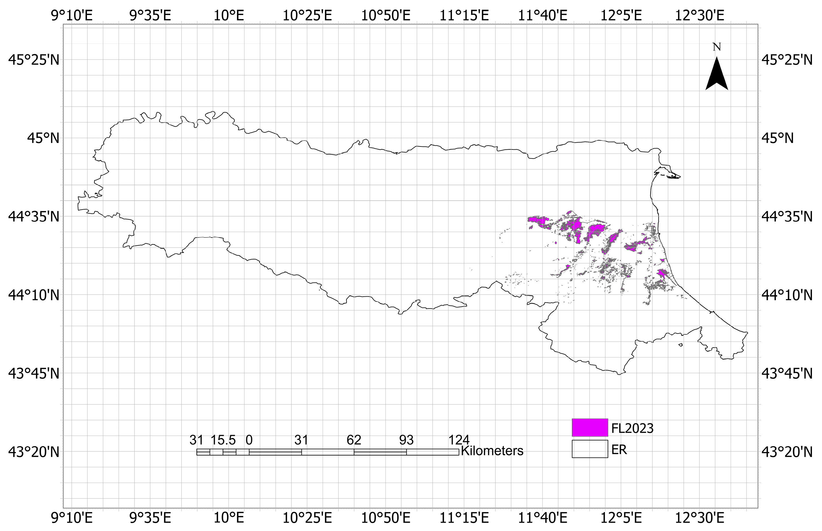
Figure 2 shows the flooded polygon of the two flooding events in Emilia-Romagna in May 2023 and the whole Emilia-Romagna region. The whole region of Emilia-Romagna is approximately 22,453 km2, of which about 48% lies in the plain (approximately 10,700 km2), while the remaining 52% is divided between hilly and mountainous areas (approximately 11,753 km2). The plain supports most of the economic and agricultural activity. The flooded area, determined by Copernicus, was approximately 321 km2, confined entirely to the plain, which is cultivated mainly with orchards and is a key agricultural zone of the region. Note that the flood-affected area reported by the regional authorities is 540 km2, and the difference is due to the mapping methodology (satellite data or filed survey).

3.1. NPP and AGB Change (2022–2023)

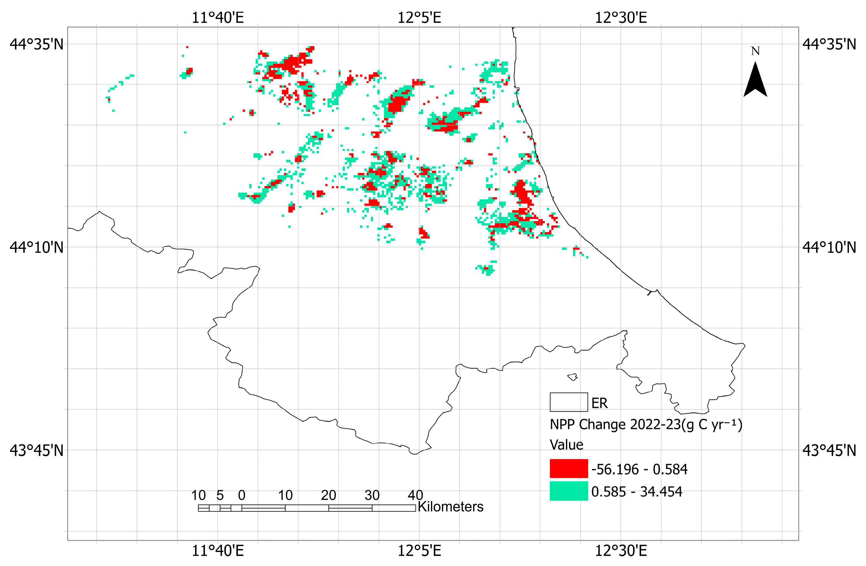
The map in Figure 3 shows how net primary production changed from 2022 to 2023 across the flooded region. Areas in red experienced a decrease in NPP, likely due to the severe impacts of flooding on vegetation and other factors. Areas in green experienced an increase in NPP, suggesting they were less negatively affected by the floods.
The data in Table 4 quantify these NPP changes for the flood-affected region and the whole Emilia-Romagna area. In the flood zone, 51.96% of the area saw a decrease in NPP, while 48.04% had an increase. However, the total NPP losses (−2.2 × 10⁴ g C yr−1) outweighed the gains (1.5 × 10⁴ g C yr−1), resulting in a net NPP deficit of −7.0 × 10³ g C yr−1 across the flooded areas. For all of Emilia-Romagna, a larger portion (54.5%) experienced NPP increases compared to decreases (44.5%). The total NPP gain of 2.7 × 10⁶ g C yr−1 exceeded the losses, leading to an overall net gain of 6.7 × 10⁵ g C yr−1 across the region. This suggests that while flooding severely impacted NPP in localized areas, much of Emilia-Romagna was productive in 2023.
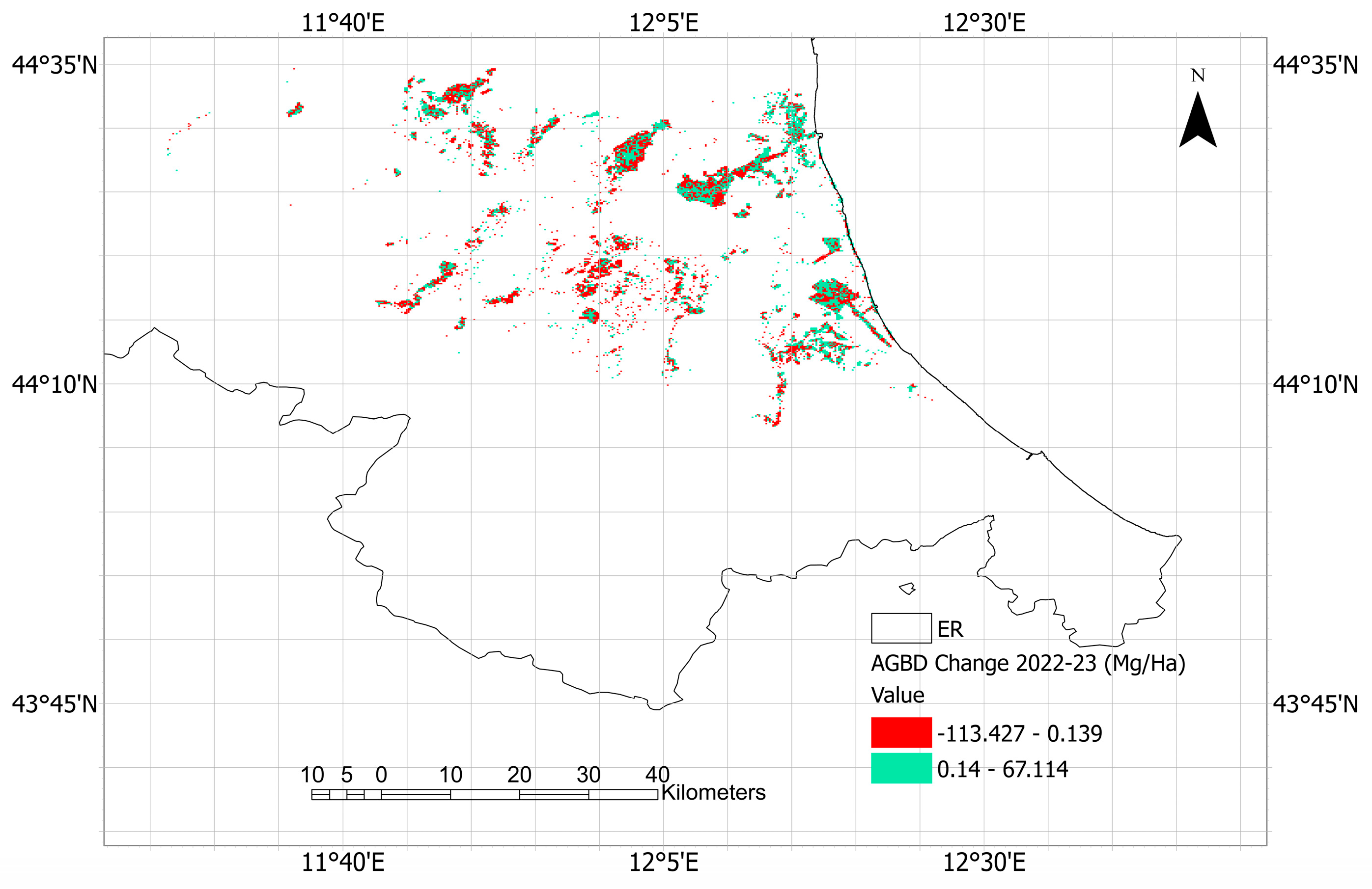
Figure 4 shows areas that decreased (red) or increased (green) AGBD from 2022 to 2023 within the flooded polygons. The red zones likely represent the most flood-impacted areas where crops, trees, or other vegetation experienced die-off or stunted growth.
Table 4 quantifies these changes: 49.4% of the flood zone saw AGB decline, while 50.6% had biomass increases. However, the total AGB losses (−1.0 × 10³ Mg C) exceeded the gains (0.5 × 10³ Mg C), resulting in a net deficit of −0.5 × 10³ Mg C across the flooded areas. Across all of Emilia-Romagna, a much larger portion (69.4%) experienced AGBD decreases compared to increases (28.04%), the remaining 2.56% of the area showed no change in AGBD. The region had a substantial total AGB loss of −3.5 × 10⁵ Mg C that far outweighed the gains of 2.8 × 10⁴ Mg C, leading to a large net AGB deficit of −3.3 × 10⁵ Mg C. This significant regional AGB loss, extending beyond just the flood zone, may reflect other factors like tree harvesting, land-use changes, drought, or landslide impacts in addition to the flooding event.
In summary, while parts of the flood zone saw changes in productivity and biomass, the overall net changes were negative within the flooded areas, likely due to the impacts of the flooding. Across Emilia-Romagna, NPP still showed an overall gain driven by productive areas, but AGB exhibited a substantial regional deficit likely stemming from a combination of flood impacts and other environmental pressures. The negative biomass change far outweighs the modest biomass gain areas, reflecting widespread tree mortality or harvest. In addition, approximately 80 km2 of Emilia-Romagna experienced landslides [43], which likely contributed to additional AGB losses.

3.2. RSEI Change (2014–2024)

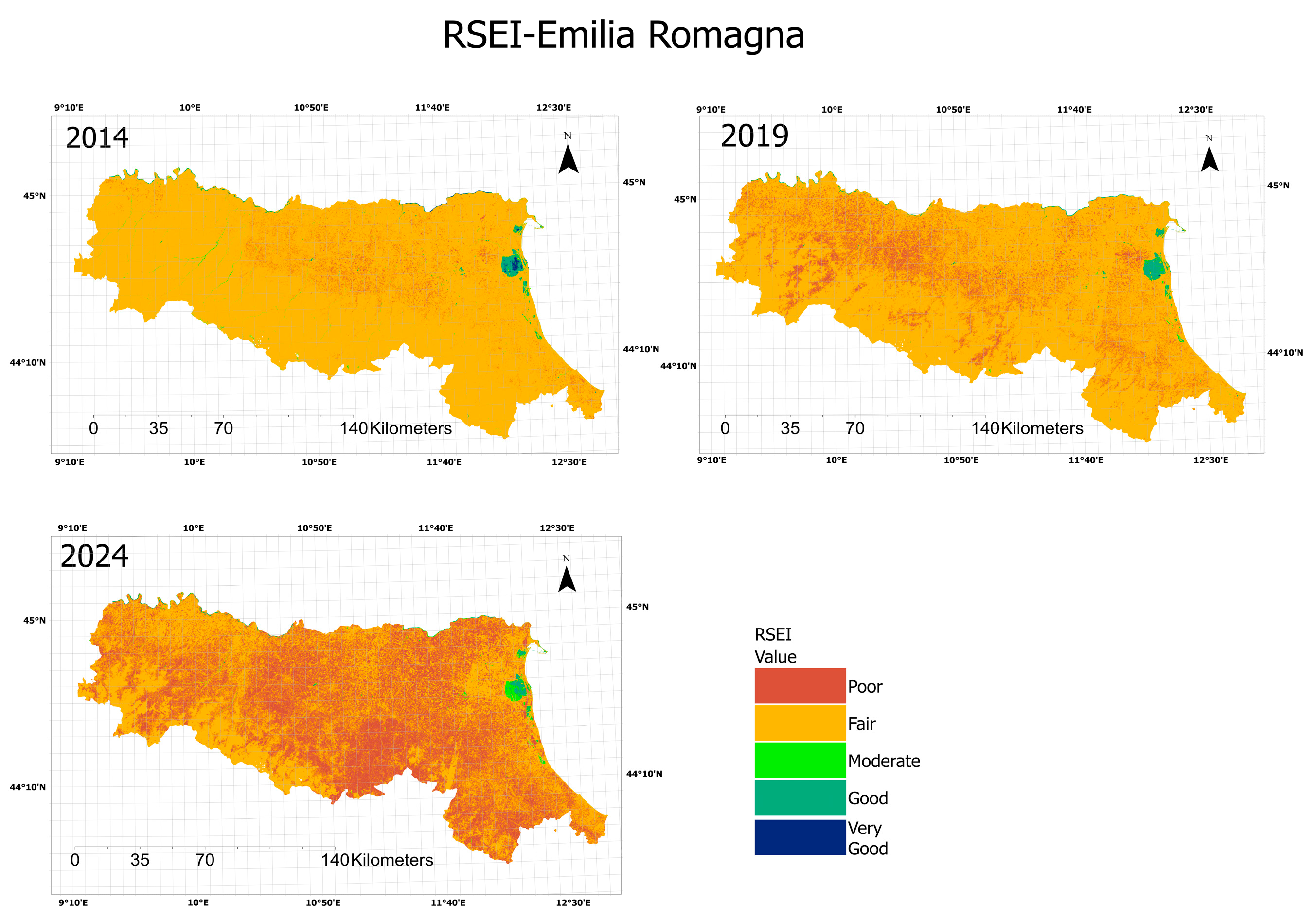
To assess changes in ecological quality over time, RSEI was evaluated for the Emilia-Romagna region and its flood-affected areas for the years 2014, 2019, and 2024 (Figure 5).
Table 5 displays the area belonging to each ecological class in the years considered, and Figure 6 plots the corresponding percentages of total area. There is a pronounced decline in ecological conditions across the region. In 2014, approximately 90% of Emilia-Romagna (20,847 km2) was classified under the Fair ecological quality class. By 2024, this share had fallen to just over 50% (11,547 km2), while the Poor category expanded dramatically from 846 km2 in 2014 to over 10,269 km2 in 2024. The area classified as Good or Very Good declined from a combined total of 202 km2 in 2014 to just 104 km2 in 2024, with the Very Good category disappearing entirely after 2019. These results indicate widespread ecological degradation, likely influenced by climate-related stressors and anthropogenic pressures.
A similar, though spatially more limited, pattern is observed in the flood-affected zones. Here, the Poor class expanded from 17 km2 in 2014 to 96 km2 in 2024, while the Fair category shrank from 301 km2 to 224 km2. Although the total area is smaller, these changes represent a substantial percentage loss, indicating that flood-impacted areas are vulnerable to ecological degradation. Figure 6 further illustrates these class distributions over time, highlighting a clear shift toward lower RSEI categories in both the whole region and the flood-affected region.
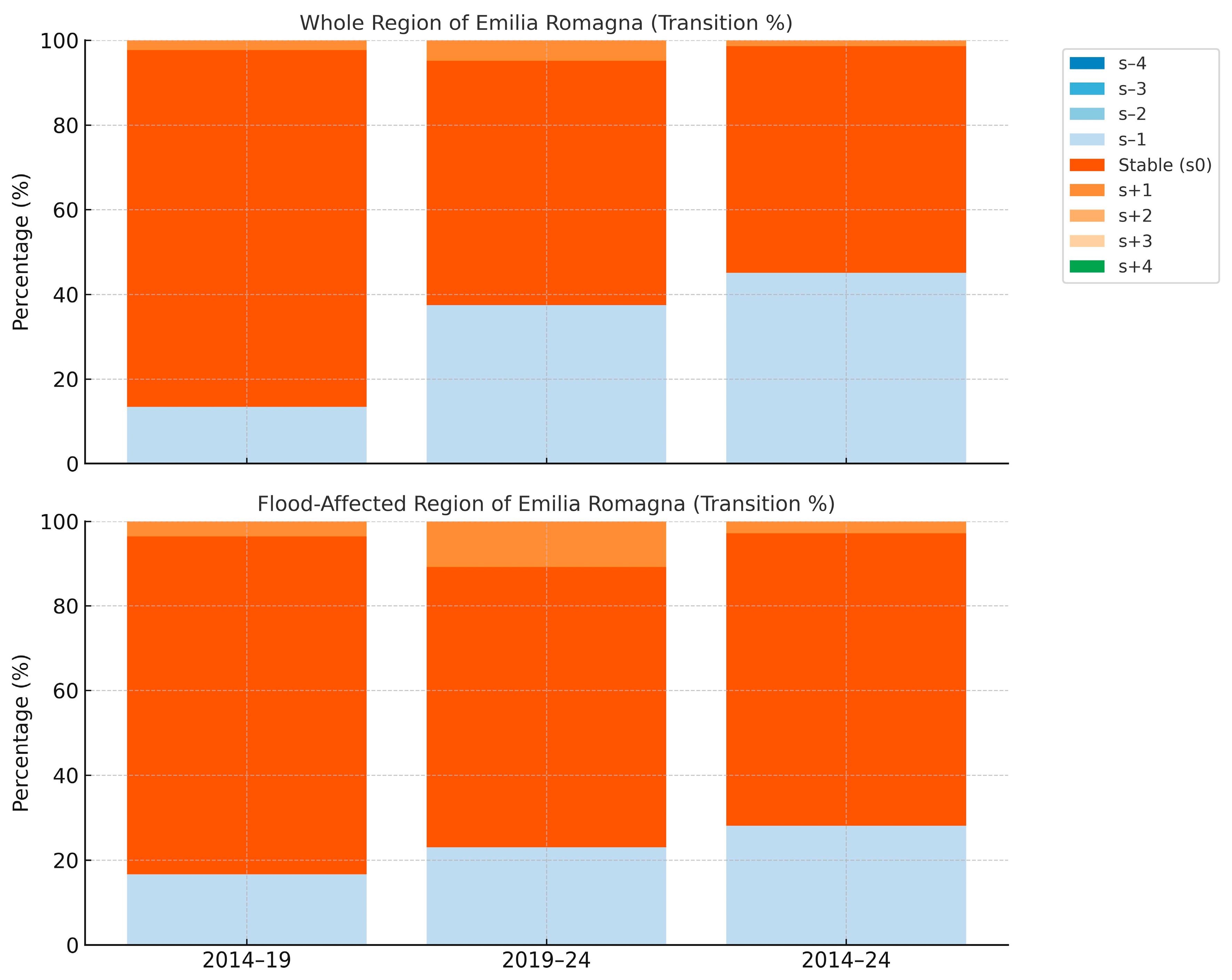
The transition analysis (Table 6 and Figure 7) further confirms these trends. Table 6 summarizes the area in km2 and the corresponding percentage over the total area of interest that showed a class transition. Figure 7 highlights the percentage distribution of RSEI classes and transitions for both the entire region and the flood-affected areas over the 10-year period. The sharper degradation observed in the latter period suggests either a change in driving factors (e.g., land-use, climate extremes, which include all three floods events) or increased ecological pressure due to the rapidly changing climate.
For the Emilia-Romagna region as a whole, the majority of the area remained ecologically stable (classified as S0) across all time intervals, exceeding 54% in each period. However, transitions indicate a clear trend of degradation, especially in recent years. During 2014–2019, approximately 2953 km2 experienced a one-level drop in ecological class (S−1), compared to just 507 km2 that improved by one level (S + 1). In the 2019–2024 period, degradation intensified with 8280 km2 dropping by one class versus only 1058 km2 improving, a nearly threefold increase in degradation compared to the previous period.
Over the entire 2014–2024 period, nearly 10,000 km2 experienced at least mild ecological decline, while only around 300 km2 saw any improvement. This indicates a net ecological loss of alarming magnitude.
In the flood-affected areas, the stability class (S0) was even more dominant, covering approximately 65% of the area throughout the study period. Nonetheless, degradation was notable from 2014 to 2024, around 80 km2 underwent ecological deterioration, while only 8 km2 improved resulting in a net loss in 72 km2. This corresponds to over 25% of the flood-affected zone experiencing a downward shift in ecological quality.
The Emilia-Romagna region and its flood-impacted areas show dramatic reductions in ecological quality, especially from 2019 to 2024. However, this degradation appears less severe in flooded areas compared to the whole region.

3.3. Total SOC and Total AGB

Previous sections showed how flooding can affect carbon stocks. In this section a quantification of SOC and AGB potentially threatened by flooding is presented.
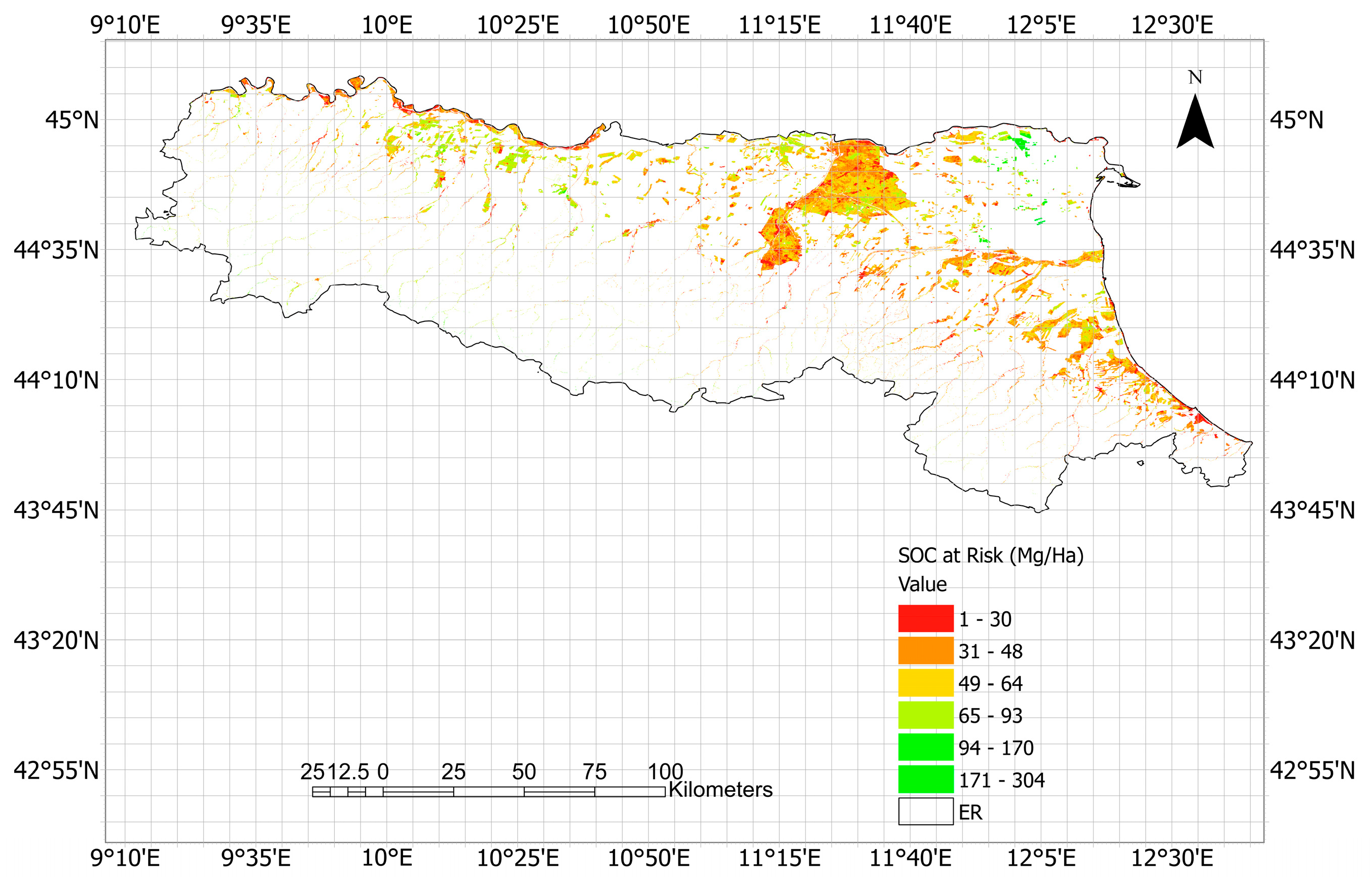
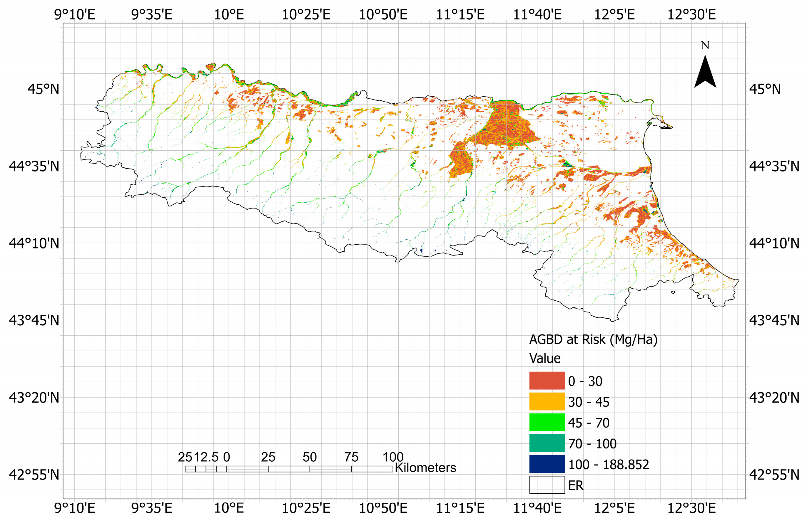
Figure 8 shows the high flood-hazard area, which is adopted from IrdoGeo [35] platform of ISPRA and used for the calculation of SOC and AGB in high-hazard zone. Higher-hazard zones may experience more frequent soil disturbances. From the calculation shown in Table 7, a considerable amount of SOC (1.1 × 10⁷ Mg C) and AGB (9.0 × 10⁶ Mg C) is found to be vulnerable to flooding in high-hazard areas, as shown in Figure 9 and Figure 10 for SOC and AGB, respectively. These values are presented with two significant digits to better reflect the uncertainties in input data and methods. If extreme flooding increases in frequency, there is a risk of losing long-term carbon stocks (both in the soil and in the standing biomass).

4. Discussion

These results collectively indicate a significant and accelerating decline in ecological quality across the region, with particularly acute effects in flooded areas. The steep rise in degraded zones and the near disappearance of high-quality ecological classes underscore a growing vulnerability of the landscape. The combined impacts of extreme weather events, such as flooding, and possibly land-use intensification, are compromising the region’s ecological resilience. This degradation has profound implications for biodiversity, carbon sequestration, water regulation, and other ecosystem services critical to climate adaptation and regional sustainability.
Flooding events can have far-reaching implications for ecosystem dynamics, particularly influencing the carbon cycle and carbon sequestration processes, especially if they are recurrent. Indeed, flooding can lead to waterlogging, reducing oxygen availability for roots, which hampers plant metabolism and growth. Over time, reduced NPP means less carbon is fixed through photosynthesis. If flooding is severe or recurrent, many plants, especially those not adapted to such conditions, might suffer and may result in a decline in AGB, diminishing the overall carbon storage potential of an ecosystem. While ecosystems have the capacity to adapt to climate change, this process requires time. The current rate of anthropogenic climate change, however, is occurring at a pace that exceeds the adaptive capacity of many ecosystems. Consequently, the resilience of ecosystems facing increased flooding frequency and intensity may be compromised, leading to long-term alterations in ecosystem structure and function, and potentially transforming carbon sinks into carbon sources [44].

4.1. Flood Impacts Across Timescales: Productivity, Ecological Quality, and Vulnerablity of Carbon Stocks

The short-term analysis based on NPP and AGB showed that, in the flood-affected region, around half the area exhibited negative NPP and AGB changes, with a net loss of approximately 7 × 10³ g C yr−1 of annual productivity and 0.5 × 10³ Mg C of standing biomass, suggesting that floodwaters may be the primary stressor. Across all of Emilia-Romagna, total NPP still showed a strong net gain (6.7 × 10⁵ g C yr−1), driven by vigorous growth in unaffected agricultural and forested lands. Yet, above-ground biomass experienced a substantial net loss (3.3 × 10⁵ Mg C), reflecting both flood-induced mortality and additional losses from landslide-impacted areas (80 km2), as reported in the study [45].
The results reveal contrasting impacts of flooding on NPP and AGB at both the flood-affected region and the broader Emilia-Romagna scale. In the flood-affected region, losses in NPP outweigh gains, resulting in a net loss in NPP. This aligns with previous findings that flooding disrupts photosynthetic activity through prolonged submersion, reduced light availability, and sediment deposition [46,47]. The net decline in productivity suggests that the immediate ecological impact of floods in such regions is dominated by biomass loss and reduced carbon assimilation capacity. Similarly, AGB shows a clear net loss in flood-affected areas, with losses nearly double the gains. This pattern reflects the physical damage caused by natural hazards like hurricanes, including uprooting, branch breakage, and mortality, which directly reduce carbon stocks aboveground, as previously observed in [48]. At the regional scale of Emilia-Romagna, NPP shows an overall net gain, despite significant losses, because gains in unaffected or recovering areas offset flood-related declines. This suggests that ecosystem resilience and spatial heterogeneity play important roles in balancing productivity at larger scales. Flooding can trigger the breakdown of both above- and below-ground biomass. In ecosystems where floods cause widespread mortality, there is an increased release of CO2 and methane as dead organic matter decomposes, shifting the area from a carbon sink to a potential carbon source. As greenhouse gas concentrations rise due to the impaired sequestration and increased release of carbon, global temperatures may continue to climb. This can, in turn, further exacerbate climate change effects and further destabilize ecosystems and their capacity to sequester carbon.
The medium-term analysis performed in terms of RSEI shows a marked decline in ecological quality in Emilia-Romagna from 2014 to 2024, with Fair areas shrinking by around 40% and Poor areas expanding. Higher-quality classes (Good and Very Good) nearly disappeared, reflecting widespread degradation driven by climate stressors and human pressures. Transition analysis highlights an acceleration of decline after 2019, with degradation compared to the previous period. Flood-affected areas follow a similar pattern, with about 25% experiencing ecological decline, though rates are somewhat lower than in the region overall. Repeated flooding likely exacerbates erosion, nutrient loss, and biomass reduction, while land-use changes and climate extremes intensify degradation [41,46,47]. The slightly slower decline in flood zones may reflect some inherent resilience of floodplain ecosystems or a lower level of anthropic disturbance. These results suggest significant, accelerating ecological loss, underscoring the urgency for integrated management to preserve ecosystem function and resilience. This finding aligns with recent studies which demonstrate that anthropogenic activities and natural hazards exert a strong influence on RSEI-derived ecological quality, see, e.g., [23,30,31,49].
Since RSEI can capture the cumulative ecological stress resulting from both anthropogenic activities and natural hazards, overlaying an RSEI change map (pre/post event or trend breaks) with an independent landslide or flood inventory may represent a valid method to attribute ecological declines to specific hazard occurrences and to quantify the affected area and severity, enabling loss estimates and recovery monitoring [32]. Overall, RSEI provides a cost-effective, repeatable, and spatially explicit method to evaluate the ecological consequences of geohazards. Its integration with geospatial hazard maps and models along with AGB, NPP, and ground-based data can enhance our understanding of the feedback loops between environmental degradation and hazard risks. However, limitations remain, particularly in differentiating short-term disturbance signals (e.g., immediate flood damage) from long-term ecological processes (e.g., vegetation succession).
Carbon stock estimates in high-hazard, flood-prone areas further underline the ecological importance of these zones. Indeed, SOC and AGB represent a substantial carbon reservoir [50]. Flood events, however, threaten these stocks through erosion, organic matter loss, and vegetation damage, thereby reducing carbon storage capacity and weakening climate regulation functions. This combination of ecological degradation and carbon stock loss underscores the vulnerability of flood-prone landscapes and highlights the urgent need for integrated management strategies that address both flood risks and ecosystem conservation.

4.2. Uncertainty and Accuracy of Results

The results presented in this study must be interpreted in light of the inherent uncertainties associated with the datasets used. Each dataset has its own accuracy limitations, stemming from sensor noise, model assumptions, and data resolution. A concise summary is presented in Table 8. Per-pixel uncertainty metadata were not available for input rasters. Where dataset-provided uncertainty values were absent, uncertainty ranges reported here were chosen based on peer-reviewed validation and assessment studies for the respective data types.
For above-ground biomass density (AGBD), the GEDI mission provides one of the most accurate spaceborne lidar products currently available. However, footprint-level and gridded estimates still show variability. Global GEDI biomass models report uncertainties of approximately ±20% at regional scales [51], while site-level validation studies in Mediterranean ecosystems have reported relative root mean square errors (RMSE) ranging from 38% to 85%, depending on forest structure [52]. These findings highlight that while GEDI provides valuable biomass data, caution is needed when interpreting results in heterogeneous or fragmented landscapes.
For soil organic carbon (SOC), uncertainties arise from limited field sampling density, interpolation methods, and spatial heterogeneity of soils. Recent studies employing conformal prediction frameworks suggest that SOC mapping uncertainties generally range between ±10–20% at regional scales [53]. These errors are acceptable for identifying broad patterns of SOC vulnerability but underline that precise site-specific SOC values cannot be guaranteed.
For digital elevation models (DEM) used in flood delineation, data at 30 m resolution are widely adopted but introduce vertical errors of ±5–10 m, which can translate into 10–15% uncertainty in flood extent predictions in low-relief areas [54]. Coastal and floodplain validation studies have further highlighted the impact of DEM errors on inundation mapping, showing positional uncertainties of up to ±5–15% m under certain conditions [55]. However, DEM was not used for flood mapping or hydrodynamic analysis in this study. Instead, the flood extent polygons were obtained from Copernicus (EMS) products; the DEM was only employed for generating AGBD maps, where such vertical uncertainty can be considered to have a minimal effect on the final outcome.
For net primary productivity (NPP), satellite-derived estimates are influenced by cloud contamination, mixed-pixel effects, and model parameterization. Evaluation against field measurements indicates uncertainties, while regional applications of the CASA model show additional error propagation from climatic variables and land-cover assumptions [56]. Global model validation efforts [57] also highlight that while large-scale aggregation reduces noise, local-scale estimates remain subject to significant uncertainty. In the case of RSEI, aggregation of multiple indices and atmospheric correction remains subject to significant uncertainty.
Table 8. Sources of uncertainty in datasets used in the study.
DatasetResolutionSourceMain Source of Error Uncertainty (%)
SOC 100 mRegione Emilia-RomagnaSoil sampling density, interpolation, heterogeneity±10–20% [53]
DEM30 mGoogle Earth EngineVertical error, vegetation cover, steep terrain±5–10 m (≈±10–15% impact on flood delineation) [54,55]
High Flood-Hazard ZonesIdroGEO–ISPRAModel assumptions, incomplete hydrological records±5–15% [55]
NPP/GPP 30 mGoogle Earth EngineCloud contamination, mixed-pixels, canopy assumptions±15–25% [56,57]
NDVI30 mGoogle Earth EngineAtmospheric effects, seasonal variability, sensor noise±10–15% [58,59]
AGBD 25 mUSGS LP DAAC/LARSELiDAR footprint gaps, canopy structure variability±20% [51,52,60]
Flood PolygonsCopernicus EMSMapping time, cloud cover, water turbidity±5–10% [61]
RSEI30 mGoogle Earth EngineAggregation of multiple indices, atmospheric correction±10–20% [62]
Taken together, these uncertainties suggest that while the absolute values of SOC, NPP, AGB, and RSEI presented here should be interpreted with caution, the overall conclusion remains robust: there is a degradation of carbon stocks, and substantial carbon pools in both soil and vegetation are located in high flood-hazard areas. If extreme flooding increases in frequency and intensity, significant long-term carbon losses from both SOC, NPP, and AGB are at risk [51,53,54].
As summarized in Table 8, the expected combined uncertainties from different datasets are on the order of ±10–20% at the regional scale. While these uncertainties affect the exact values, they do not alter the overall conclusion that flooding is affecting ecosystem dynamics both in short- and long-term to a certain extent and could influence substantial SOC and AGB pools concentrated within high-hazard flood zones if extreme events increase under climate change scenarios in the future.

4.3. Limitations of the Study

Although this study integrates multiple remote sensing datasets and validated sources, several limitations should be acknowledged. First, there is a resolution mismatch between datasets (e.g., SOC at 100 m vs. GEDI AGBD at 25 m and Landsat products at 30 m). This may introduce aggregation errors when aligning datasets for analysis in flood-hazard zones.
Second, temporal mismatches exist among the datasets used. For example, flood-hazard polygons from Copernicus EMS represent specific extreme events, while SOC and AGB are long-term averages, and NPP varies seasonally. This discrepancy limits the ability to capture short-term dynamics of carbon loss under flooding.
Third, uncertainties from input datasets are compounded when calculating derived quantities such as total SOC or AGB vulnerable to flooding. While Table 8 summarizes individual dataset uncertainties, the combined propagation of error may be significant, particularly in heterogeneous landscapes. Fourth, the analysis does not include comprehensive ground validation due to the regional scale of the study. While SOC and AGB estimates are consistent with published values, the absence of field plots or soil cores for direct comparison limits validation strength.
Finally, the hazard zones derived from IdroGEO (ISPRA) are based on hydrological modeling assumptions and historical flood records. These hazard maps may not fully capture future changes under climate change scenarios, potentially underestimating flood hazards.
Despite these limitations, the integration of multiple datasets and cross-validation with published uncertainty ranges provides confidence that the main conclusion remains robust, significant carbon stocks in both soil and vegetation are exposed to high flood-hazard risk, making them vulnerable to long-term loss under more frequent extreme flood events.

4.4. Future Work

Future studies should aim to reduce the limitations highlighted above by incorporating higher-resolution datasets and multi-temporal analyses. For instance, missions such as NASA NISAR and ESA BIOMASS are expected to provide improved AGB estimates at finer spatial scales, which could reduce uncertainty compared to current GEDI-based products. Similarly, the integration of LiDAR- and UAV-based surveys could provide localized calibration points for both SOC and AGB, helping to validate satellite-derived estimates.
Another priority is the development of temporally consistent datasets. Seasonal variations in NPP/GPP and SOC dynamics could be better captured by integrating time-series data from MODIS, Sentinel-2, and other platforms with higher revisit frequencies, ensuring that short-term flood events and seasonal carbon fluxes are adequately represented.
In terms of flood mapping, higher-accuracy DEMs (e.g., TanDEM-X, LiDAR-based topography) and up-to-date satellite altimetry like ICESat-2 could substantially improve flood extent delineation. Moreover, incorporating climate change-adjusted flood-hazard scenarios would provide a more realistic estimate of long-term risks, especially in regions where extreme weather events are projected to intensify.
Finally, a stronger emphasis on ground validation is essential. Establishing field plots for biomass and soil sampling campaigns would not only strengthen accuracy assessments but also facilitate the calibration of regional models. Collaboration with local environmental agencies and soil monitoring networks could provide the necessary ground data to improve regional estimates of carbon stocks under flood risk.
By combining improved datasets, advanced modeling techniques, and targeted ground validation, future work can significantly enhance the accuracy of SOC and AGB assessments, leading to more robust evaluations of carbon vulnerability in flood-prone landscapes.
Although uncertainties in input datasets and methods may affect the absolute values reported, the relative magnitude and spatial concentration of SOC and AGB within high-hazard zones remain consistent, supporting the robustness of our main conclusions.

5. Conclusions

This study presents an integrated assessment of the impacts of flooding on ecosystem productivity, carbon storage, and ecological quality in the Emilia-Romagna region of Italy, which has been hit by major flooding events in 2023. The key findings indicate significant reductions in NPP and AGB within flood-affected areas, translating into a net loss of carbon sequestration potential. The analysis over a decade of RSEI further revealed a concerning trend of widespread ecological degradation across the region. In addition, a quantification of AGB and SOC in high flood-hazard zones reveals that a significant amount of carbon is stored and threatened by these events.
Notably, the combined effects of flooding and landslides in Emilia-Romagna resulted in a meaningful depletion of carbon stocks, underscoring the importance of integrating multiple disturbance pathways in carbon accounting and land management strategies. Effective ecosystem management and climate adaptation plans will be essential to build resilience, offset some of these impacts, and maintain the critical role that natural systems play in mitigating climate change through carbon sequestration.
As the frequency and intensity of extreme weather events continue to rise under a changing climate, proactive measures to protect and restore vulnerable ecosystems will become increasingly crucial. Integrating flood risk assessments with ecosystem monitoring and carbon dynamics analysis can inform targeted interventions, such as riparian restoration, soil conservation practices, and sustainable land-use planning. Such integrated approaches can help safeguard vital ecosystem services, enhance carbon storage capacity, and contribute to regional climate change mitigation and adaptation efforts.
While providing valuable insights, this study has certain limitations, as the remote sensing approach lacks comprehensive field observations for full validation. The analysis also lacks long-term field observations, which are essential to understand both immediate impacts and longer-term recovery from recurrent flooding events. These results should be interpreted as indicative estimates rather than exact values, as they are subject to the uncertainties discussed above; nevertheless, they clearly demonstrate the magnitude of carbon stocks that may be at risk in high flood-hazard zones. Addressing these limitations through future research integrating field data will enhance our understanding of how floods influence ecosystem processes and improve the reliability of predictions related to the carbon cycle and sequestration in flood-prone regions.

Author Contributions

Conceptualization, J.Q. and F.C.; methodology, J.Q.; software, J.Q.; validation, J.Q.; writing—original draft preparation, J.Q. and F.C.; writing—review and editing, J.Q. and F.C.; visualization, J.Q. and F.C.; supervision: F.C.; funding acquisition, F.C. All authors have read and agreed to the published version of the manuscript.

Funding

This study was funded by the European Union—NextGenerationEU, Mission 4, Component 2, in the framework of the GRINS-Growing Resilient, INclusive and Sustainable project (GRINS PE00000018—(GRINS PE00000018—CUP C93C22005270001). The views and opinions expressed are solely those of the authors and do not necessarily reflect those of the European Union, nor can the European Union be held responsible for them.

Data Availability Statement

The original contributions presented in this study are included in the article. Further inquiries can be directed to the corresponding authors.

Conflicts of Interest

The authors declare no conflicts of interest.

Appendix A

This appendix provides a brief description of the model from which the data were derived for SOC, AGBD, and NPP.

Appendix A.1. Net Primary Productivity (NPP)

The methodological framework used to compute NPP follows [63], that calculates NPP at a location x and time t with the CASA model, that is a variant of the light use efficiency (LUE) model originally proposed by Monteith (1972) [64] (Equation (A1)).
NPP (measured in gC m−2 yr−1) is calculated as the product of photosynthetically active radiation (PAR), the fraction of PAR absorbed by vegetation (FPAR), and the conversion efficiency (ε):
NPP(x,t) = PAR(x,t) × FPAR(x,t) × ε(x,t)
PAR is computed as follows:
PAR(x,t) = SOL(x,t) × 0.5
where SOL(x,t) is global solar radiation (MJ m−2 d−1) from ERA5 reanalysis, and 0.5 represents the fraction of PAR [65].
FPAR is computed from NDVI data as
FPAR = NDVI × 1.2 − 0.14
ε is expressed as follows:
ε(x,t) = εmax × Tε1(x,t) × Tε2(x,t) × Wε(x,t)
where εmax is the maximum conversion efficiency, obtained via regression between field dry matter and absorbed PAR (APAR), then converted to carbon rates following [66], Tε1 and Tε2 are temperature stress coefficients, and Wε is the water stress coefficient [67].
Absorbed PAR (APAR) is derived as follows:
APAR(x,t) = SOL(x,t) × FPAR(x,t) × 0.5
The temperature stress coefficients are calculated using a parabolic temperature response function centered at an optimal temperature (Topt).
The water stress coefficient is derived from a formulation based on the Temperature Vegetation Dryness Index (TVDI) [68]:
WεTVDI = 1 − (TVDI × 0.5)
TVDI was calculated from the Ts–NDVI space (Equation (A7)), where Tsmin defines the wet edge, and parameters a and b describe the dry edge.
TVDI = (Ts − Tsmin)/(a + b × NDVI − Tsmin)
The TVDI-derived Wε well captures spatial variability in NPP, enhancing geospatial accuracy when combined with remotely sensed data.
The implementation of this methodological workflow in GEE consists of the following steps:
1.
Input Data Preparation:
Four primary satellite-based ImageCollections were used as inputs: the LANDSAT collection, available on GEE, was used to compute the NDVI and LST. This dataset provides a spatial resolution of 30 m. Cloud masking was performed using the QA_PIXEL bitmask to eliminate pixels affected by clouds and cloud shadows.
Additionally, ERA5-Land data provided by the ECMWF (European Center for Medium-Range Weather Forecasts) were used to estimate SOL, which served as a proxy for APAR. ERA5-Land data have an approximate spatial resolution of 11.132 km and were accessed through the Earth Engine Data Catalog.
NDVI was computed from the red and near-infrared reflectance bands, while LST was derived from the thermal band and converted from Kelvin to degrees Celsius. Water stress coefficient (Wε) was estimated using the Temperature Vegetation Dryness Index (TVDI). The temperature scalar (Tε) was calculated using a parabolic temperature response function centered at an optimal temperature (Topt) of 21.66 °C. Additionally, two static inputs were considered: the region of interest (ROI) represented as a FeatureCollection Emila-Romagna, the maximum light use efficiency (LUEmax = 0.72) as a scalar constant, and the optimum temperature (Topt) as a scalar.
2.
Pre-processing:
All input ImageCollections were clipped to the ROI using the ‘clip (ROI)’ function. The datasets were then resampled using the reproject () function to ensure spatial consistency across layers.
3.
Computation of NPP:
NPP is calculated using Equation (A1), where the terms are derived as explained in Equations (A2)–(A7).
4.
Output:
The resulting NPP values were exported as ImageCollections, which represented spatially explicit maps of NPP for the study area. This framework enables consistent and scalable estimation of NPP across spatial domains by integrating remotely sensed variables with a light use efficiency approach.

Appendix A.2. Above-Ground Biomass Density (AGBD)

AGBD is one of the products of the Global Ecosystem Dynamics Investigation (GEDI) [36]. GEDI is a multibeam lidar instrument aboard the International Space Station (ISS), designed to measure vegetation height and quantify aboveground carbon stocks in temperate and tropical forests and woodlands. GEDI04_A provides AGBD estimates for individual footprints along with associated prediction intervals. The algorithm employs relative height (RH) metrics from GEDI02_A and 13 linear models to predict AGBD across 32 combinations of plant functional type (PFT) and world region within the ISS observation limits. It describes the scientific and mathematical assumptions required to generate globally representative AGBD estimates, including extrapolation beyond training data and the exclusion of GEDI02_A observations not meeting algorithm requirements [69,70]. The resulting footprint-level predictions provide global coverage of AGBD and form the basis for the gridded GEDI04_B product.
In the present study, we utilize data from NASA’s GEDI mission to calculate AGBD. GEDI’s lidar measurements, combined with Sentinel-2 satellite imagery and elevation models, are employed to train a regression model for biomass prediction. The methodology aims to quantify AGBD and total AGB adopted from [69]. For this purpose, GEDI lidar measurements, acquired at a spatial resolution of 30 m, are used as reference data capturing vertical vegetation structure. Sentinel-2 data, including spectral bands and vegetation indices, are processed into annual cloud-free composites using Google’s Cloud Score dataset. Elevation and slope information from the Copernicus GLO-30 DEM are incorporated for both pre-processing and as model predictors.
Data preparation includes filtering, scaling, and mosaicking. GEDI data are screened to remove low-quality observations based on flags, relative error, and slope criteria, while Sentinel-2 composites are derived using median pixel values. All datasets are exported as assets to address computational limitations. The regression model is built using Sentinel-2 variables, elevation, and slope as predictors, with GEDI AGBD serving as the dependent variable. Resampling and stratified sampling techniques ensure spatial alignment and sufficient coverage of valid data points.
The trained regression model produces AGBD predictions, which are subsequently used to estimate total AGB. Non-vegetated pixels are excluded using the ESA World Cover dataset, and total AGB is calculated by multiplying predicted AGBD values by pixel area and summing across the study region. Estimates are generated for both 2022 and 2023. All analyses are conducted within the Google Earth Engine (GEE) environment.

Appendix A.3. Remote Sensing Ecological Index (RSEI)

This study constructs the RSEI of the study area using greenness, humidity, dryness, and heat based on cloud-minimized synthetic images during the vegetation growth season of the target year via the GEE platform. The RSEI integrates multiple environmental indicators into a single composite index to assess ecological quality [41,71]
  • The RSEI components are defined as follows:
    • Greenness: expressed by NDVI.
    • Wetness: represented by the humidity component from Tasseled Cap Transformation (TCW).
    • Dryness: measured by NDBSI (Normalized Difference Built-up and Soil Index), which combines the Building Index (IBI) and Soil Index (SI).
  • Heat: represented by land surface temperature (LST).
To avoid subjective bias in weighting, the Principal Component Analysis (PCA) method is applied to concentrate the main information of the four indicators into the first principal component. Before PCA, all indicators are normalized to a range of 0–1:
NIi = (Ii − Imin)/(Imax − Imin)
where (NIi) is the normalized value of the index; Ii is the initial pixel value of the component index; (Imin) and (Imax) are the minimum and maximum values of the component index, respectively.
The initial RSEI0 is obtained via PCA of the four normalized indicators:
RSEI0 =1 − PC1(NINDVI, NILST, NINDBSI, NIWET)
Finally, to enable comparison across different periods, RSEI0 is normalized to produce the final RSEI:
RSEI = (RSEI0 − RSEI (0, min))/(RSEI(0, max) − RSEI(0,min))
Here, RSEI ranges from 0 to 1, where higher values indicate better ecological quality and lower values indicate poorer ecological quality.

Appendix A.4. SOC

The methodology was applied to estimate soil organic carbon (SOC) stocks in the plains and the Apennines. Conditional geostatistical simulations, tailored to the variables considered, were used to generate the following maps (CNR Report, October 2015 [72]):
  • Organic carbon content (%) in the 0–30 cm soil layer.
  • Soil texture (sand, silt, clay, skeleton, textural class) in the 0–30 cm layer.
These outputs, represented on a 100 m grid, were used to calculate SOC stock. The calculation, expressed in Mg C ha−1, requires bulk density (BD, Mg m−3). BD was estimated using a pedotransfer function (PTF) based on granulometric fractions, organic carbon content, and skeleton fraction, corrected for skeleton in the top 30 cm. The PTF [72], calibrated with Evolutionary Polynomial Regression [73], was applied to 44,052 grid cells. For 2704 cells with C org ≥ 2.5%, an alternative PTF [74] was used:
BDOrg = 1.4903 − 0.33293 × Ln (C org %)
Apparent density values were further corrected for skeleton content, based on observations from 6785 sites (fskel-skeleton fraction, 0–70%). Only 31 cells, with skeleton ≥ 10%, required correction [75]. The resulting fine-earth bulk density (BDfc) was used to compute SOC stock per hectare:
Cstock = (1 − fskel) × C org% × 30 × BDfc × 100
SOC stock was then converted to CO2 equivalents:
CO 2 eq   =   C stock   ×   ( 44 12 )
SOC values refer to a 30 cm depth and a surface unit of 1 ha (10,000 m2). However, since grid cells may include non-soil areas (urban, gullies, beaches, salt marshes, etc.) or extend beyond the region, the effective soil-covered area was refined using the 2017/2020 Land-Use Map (1:25,000 scale) and additional work by Corticelli S. et al. (2008) [76] who attributed to each category of the land-use map.

References

  1. Richie, H.; Rosado, P.; Roser, M. Natural Disasters. OurWorldInData.org. Available online: https://ourworldindata.org/natural-disasters (accessed on 13 April 2025).
  2. Wahlstrom, M.; Guha-Sapir, D. The Human Cost of Weather-Related Disasters 1995–2015; UNISDR: Geneva, Switzerland, 2015. [Google Scholar]
  3. Guddo, S. Conceptualization of Flooding Disaster: A Theoretical Perspective of Management. Disaster Adv. 2024, 17, 40–45. [Google Scholar] [CrossRef]
  4. Woldemeskel, F.; Sharma, A. Should Flood Regimes Change in a Warming Climate? The Role of Antecedent Moisture Conditions. Geophys. Res. Lett. 2016, 43, 7556–7563. [Google Scholar] [CrossRef]
  5. Archer, D.R.; Fowler, H.J. Characterising Flash Flood Response to Intense Rainfall and Impacts Using Historical Information and Gauged Data in Britain. J. Flood Risk Manag. 2015, 11, S121–S133. [Google Scholar] [CrossRef]
  6. IPCC. Climate Change Information for Regional Impact and for Risk Assessment. Climate Change 2021: The Physical Science Basis; IPCC: Geneva, Switzerland, 2021.
  7. Ji, P.; Yuan, X.; Jiao, Y.; Wang, C.; Han, S.; Shi, C. Anthropogenic Contributions to the 2018 Extreme Flooding over the Upper Yellow River Basin in China. Bull. Am. Meteorol. Soc. 2020, 101, S89–S94. [Google Scholar] [CrossRef]
  8. Sun, Q.; Zhang, X.; Zwiers, F.; Westra, S.; Alexander, L.V. A Global, Continental, and Regional Analysis of Changes in Extreme Precipitation. J. Clim. 2021, 34, 243–258. [Google Scholar] [CrossRef]
  9. Wasko, C.; Nathan, R. Influence of Changes in Rainfall and Soil Moisture on Trends in Flooding. J. Hydrol. 2019, 575, 432–441. [Google Scholar] [CrossRef]
  10. Slater, L.J.; Singer, M.B.; Kirchner, J.W. Hydrologic versus Geomorphic Drivers of Trends in Flood Hazard. Geophys. Res. Lett. 2015, 42, 370–376. [Google Scholar] [CrossRef]
  11. Kim, B.; Sanders, B.F. Dam-Break Flood Model Uncertainty Assessment: Case Study of Extreme Flooding with Multiple Dam Failures in Gangneung, South Korea. J. Hydraul. Eng. 2016, 142, 05016002. [Google Scholar] [CrossRef]
  12. Knighton, J.; Conneely, J.; Walter, M.T. Possible Increases in Flood Frequency Due to the Loss of Eastern Hemlock in the Northeastern United States: Observational Insights and Predicted Impacts. Water Resour. Res. 2019, 55, 5342–5359. [Google Scholar] [CrossRef]
  13. Rogger, M.; Agnoletti, M.; Alaoui, A.; Bathurst, J.C.; Bodner, G.; Borga, M.; Chaplot, V.; Gallart, F.; Glatzel, G.; Hall, J.; et al. Land Use Change Impacts on Floods at the Catchment Scale: Challenges and Opportunities for Future Research. Water Resour. Res. 2017, 53, 5209–5219. [Google Scholar] [CrossRef] [PubMed]
  14. Krug, A.; Primo, C.; Fischer, S.; Schumann, A.; Ahrens, B. On the Temporal Variability of Widespread Rain-on-Snow Floods. Meteorol. Z. 2020, 29, 147–163. [Google Scholar] [CrossRef]
  15. Teufel, B.; Sushama, L.; Huziy, O.; Diro, G.T.; Jeong, D.I.; Winger, K.; Garnaud, C.; de Elia, R.; Zwiers, F.W.; Matthews, H.D.; et al. Investigation of the Mechanisms Leading to the 2017 Montreal Flood. Clim. Dyn. 2019, 52, 4193–4206. [Google Scholar] [CrossRef]
  16. Psistaki, K.; Tsantopoulos, G.; Paschalidou, A.K. An Overview of the Role of Forests in Climate Change Mitigation. Sustainability 2024, 16, 6089. [Google Scholar] [CrossRef]
  17. Zhang, Y.; Zhang, X.; Fang, W.; Cai, Y.; Zhang, G.; Liang, J.; Chang, J.; Chen, L.; Wang, H.; Zhang, P.; et al. Carbon Sequestration Potential of Wetlands and Regulating Strategies Response to Climate Change. Environ. Res. 2025, 269, 120890. [Google Scholar] [CrossRef]
  18. Sha, Z.; Bai, Y.; Li, R.; Lan, H.; Zhang, X.; Li, J.; Liu, X.; Chang, S.; Xie, Y. The Global Carbon Sink Potential of Terrestrial Vegetation Can Be Increased Substantially by Optimal Land Management. Commun. Earth Environ. 2022, 3, 8. [Google Scholar] [CrossRef]
  19. Aldardasawi, A.; Eren, B. Floods and Their Impact on the Environment. Acad. Perspect. Procedia 2021, 4, 42–49. [Google Scholar] [CrossRef]
  20. Pradhan, B.; Lee, S.; Dikshit, A.; Kim, H. Spatial Flood Susceptibility Mapping Using an Explainable Artificial Intelligence (XAI) Model. Geosci. Front. 2023, 14, 101625. [Google Scholar] [CrossRef]
  21. Peng, Y.; Welden, N.A.; Renaud, F.G. Ecosystem-Based Adaptation Strategies to Multi-Hazard Risk Reduction and Policy Implications in the Pearl River and Yangtze River Deltas, China. Int. J. Disaster Risk Reduct. 2025, 116, 105053. [Google Scholar] [CrossRef]
  22. Zhao, Q.; Yu, L.; Li, X.; Peng, D.; Zhang, Y.; Gong, P. Progress and Trends in the Application of Google Earth and Google Earth Engine. Remote Sens. 2021, 13, 3778. [Google Scholar] [CrossRef]
  23. Xiong, Y.; Xu, W.; Lu, N.; Huang, S.; Wu, C.; Wang, L.; Dai, F.; Kou, W. Assessment of Spatial–Temporal Changes of Ecological Environment Quality Based on RSEI and GEE: A Case Study in Erhai Lake Basin, Yunnan Province, China. Ecol. Indic. 2021, 125, 107518. [Google Scholar] [CrossRef]
  24. Yuan, C.; Gong, P.; Bai, Y. Performance Assessment of ICESat-2 Laser Altimeter Data for Water-Level Measurement over Lakes and Reservoirs in China. Remote Sens. 2020, 12, 770. [Google Scholar] [CrossRef]
  25. Kaya, Y. Evaluation of ICESat-2 Laser Altimetry for Inland Water-Level Estimation and Reservoir Monitoring. Water 2025, 17, 1098. [Google Scholar] [CrossRef]
  26. Musaeus, A.F.; Kittel, C.M.M.; Luchner, J.; Frias, M.C.; Bauer-Gottwein, P. Hydraulic River Models from ICESat-2 Elevation and Water Observations. Water Resour. Res. 2024, 60, e2023WR036428. [Google Scholar] [CrossRef]
  27. Vatandaşlar, C.; Bolat, F.; Abdikan, S.; Pamukçu-Albers, P.; Satıral, C. Modeling Aboveground Carbon in Flooded Forests Using Synthetic Aperture Radar Data: A Case Study from Turkish Thrace. iForest 2024, 17, 277–285. [Google Scholar] [CrossRef]
  28. Satriano, V.; Ciancia, E.; Pergola, N.; Tramutoli, V. A First Extension of the Robust Satellite Technique RST-FLOOD to Sentinel-2 Data for the Mapping of Flooded Areas: The Case of the Emilia Romagna (Italy) 2023 Event. Remote Sens. 2024, 16, 3450. [Google Scholar] [CrossRef]
  29. Arrighi, C.; Domeneghetti, A. On the Environmental Impacts of the 2023 Floods in Emilia-Romagna. Nat. Hazards Earth Syst. Sci. 2024, 24, 673–678. [Google Scholar] [CrossRef]
  30. Chen, M.; Tang, C.; Yang, Y.; Xiong, J. Quantifying spatio-temporal changes in the ecological environment quality and their implications for surface mass movement after a high-magnitude earthquake. Glob. Ecol. Conserv. 2025, 58, e03454. [Google Scholar] [CrossRef]
  31. Cui, P.; Lin, Y.-M.; Chen, C. Destruction of vegetation due to geo-hazards and its environmental impacts in the Wenchuan earthquake areas. Ecol. Eng. 2012, 44, 61–69. [Google Scholar] [CrossRef]
  32. Cremonini, L.; Randi, P.; Fazzini, M.; Nardino, M.; Rossi, F.; Georgiadis, T. Causes and Impacts of Flood Events in Emilia-Romagna (Italy) in May 2023. Land 2024, 13, 1800. [Google Scholar] [CrossRef]
  33. Hawes, J.E.; Peres, C.A.; Riley, L.B.; Hess, L.L. Landscape-scale variation in structure and biomass of Amazonian seasonally flooded and unflooded forests. For. Ecol. Manag. 2012, 281, 163–176. [Google Scholar] [CrossRef]
  34. Bratt, A.; Casagli, N.; Marani, M.; Mercogliano, P.; Motta, R. Rapporto Della Commissione Tecnico-Scientifica Sugli Eventi Meteorologici Estremi di Maggio 2023; Regione Emilia-Romagna, 2023. Available online: https://www.regione.emilia-romagna.it/alluvione/rapporto-della-commissione-tecnico-scientifica/20231212_rapporto_commissione_rer.pdf (accessed on 13 April 2025).
  35. ISPRA. IdroGEO: Hazard and Risk. Available online: https://idrogeo.isprambiente.it (accessed on 15 May 2025).
  36. GEDI L4A Footprint Level Aboveground Biomass Density, Version 2.1. Available online: https://daac.ornl.gov/GEDI/guides/GEDI_L4A_AGB_Density_V2_1.html (accessed on 15 April 2025).
  37. ECMWF ERA5-Land Daily Aggregates. Accessed through Google Earth Engine. Available online: https://developers.google.com/earth-engine/datasets/catalog/ECMWF_ERA5_LAND_DAILY_AGGR (accessed on 5 April 2025).
  38. USGS. Landsat Collection 2 Level-2 Science Products. Available online: https://www.usgs.gov/landsat-missions/landsat-collection-2-level-2-science-products (accessed on 27 April 2025).
  39. Regione Emilia-Romagna. Open Data Catalogue. 2023. Available online: https://datacatalog.regione.emilia-romagna.it/catalogCTA/dataset/r_emiro_2023-08-09t162508 (accessed on 27 September 2025).
  40. da Luz, L.B. Google Earth Engine Open-Source Code for NPP. Available online: https://github.com/luanabeckerdaluz/NPPalgorithm (accessed on 15 May 2025).
  41. Yan, Y.; Zhuang, Q.; Zan, C.; Ren, J.; Yang, L.; Wen, Y.; Zeng, S.; Zhang, Q.; Kong, L. Using the Google Earth Engine to Rapidly Monitor Impacts of Geohazards on Ecological Quality in Highly Susceptible Areas. Ecol. Indic. 2021, 132, 108258. [Google Scholar] [CrossRef]
  42. Organic Carbon Stored in Regional Soils of Emilia Romagna, minERva Portal (Application Maps—Organic Carbon Stored in Regional Soils Between 0–30 cm—Third edition—Dataset—minERva. Available online: https://ambiente.regione.emilia-romagna.it/it/geologia/suoli/proprieta-e-qualita-dei-suoli/carbonio-organico-immagazzinato-nei-suoli (accessed on 15 May 2025).
  43. Regione Emilia-Romagna. Alluvione Maggio 2023—Dissesti di Versante. Available online: https://www.regione.emilia-romagna.it/alluvione (accessed on 15 May 2025).
  44. IPCC. Climate Change 2022: Impacts, Adaptation, and Vulnerability. Contribution of Working Group II to the Sixth Assessment Report of the Intergovernmental Panel on Climate Change; Pörtner, H.-O., Roberts, D.C., Tignor, M., Poloczanska, E.S., Mintenbeck, K., Alegría, A., Craig, M., Langsdorf, S., Löschke, S., Möller, V., et al., Eds.; Cambridge University Press: Cambridge, UK; New York, NY, USA, 2022; p. 3056. [Google Scholar] [CrossRef]
  45. Qadri, J.; Ceccato, F. Exploring the Interaction Between Landslides and Carbon Stocks in Italy. Sustainability 2024, 16, 11273. [Google Scholar] [CrossRef]
  46. Talbot, C.J.; Bennett, E.M.; Cassell, K.; Hanes, D.M.; Minor, E.C.; Paerl, H.; Raymond, P.A.; Vargas, R.; Vidon, P.G.; Wollheim, W.; et al. The impact of flooding on aquatic ecosystem services. Biogeochemistry 2018, 141, 439–461. [Google Scholar] [CrossRef] [PubMed]
  47. Hiraga, Y.; Amano, A.; Kazama, S. Impacts of flooding on Net Primary Productivity in the floodplain being affected by anthropic pressures. In Proceedings of the 20th IAHR APD Congress, Colombo, Sri Lanka, 28–31 August 2016. [Google Scholar]
  48. Bueno, I.T.; Silva, C.A.; Hamamura, C.; Donovan, V.M.; Sharma, A.; Qiu, J.; Xia, J.; Brock, K.M.; Schlickmann, M.B.; Atkins, J.W.; et al. Aboveground biomass density maps for post-hurricane Ian forest monitoring in Florida. Sci. Data 2025, 12, 1189. [Google Scholar] [CrossRef] [PubMed]
  49. Lin, Z.; Xu, H.; Yao, X.; Zhu, Z. Assessment and simulation of eco-environmental quality changes in rapid rural urbanization: Xiong’an New Area, China. Sci. Rep. 2024, 14, 73487. [Google Scholar] [CrossRef]
  50. Alvarez-Castellanos, M.P.; Escudero-Campos, L.; Mongil-Manso, J.; San Jose, F.J.; Jiménez-Sánchez, A.; Jiménez-Ballesta, R. Organic Carbon Storage in Waterlogging Soils in Ávila, Spain: A Traditional Agrosilvopastoral Region. Land 2024, 13, 1630. [Google Scholar] [CrossRef]
  51. Duncanson, L.; Kellner, J.; Armston, J.; Dubayah, R.; Healey, S.P.; Patterson, P.L.; Saarela, S.; Marselis, S.; Silva, C.; Tang, H.; et al. Aboveground Biomass Density Models for NASA’s Global Ecosystem Dynamics Investigation (GEDI) Lidar Mission. Remote Sens. Environ. 2022, 270, 112845. [Google Scholar] [CrossRef]
  52. Dorado-Roda, I.; Martín-Alcón, S.; Brotons, L.; Coll, L. Assessing the Accuracy of GEDI Data for Canopy Height and AGB Models in Mediterranean Ecosystems. Remote Sens. 2021, 13, 2279. [Google Scholar] [CrossRef]
  53. Kakhani, N.; Alamdar, S.; Kebonye, N.M.; Amani, M.; Scholten, T. Uncertainty Quantification of Soil Organic Carbon Estimation from Remote Sensing Data with Conformal Prediction. Remote Sens. 2024, 16, 438. [Google Scholar] [CrossRef]
  54. Uuemaa, E.; Ahi, S.; Montibeller, B.; Muru, M.; Kmoch, A. Vertical Accuracy of Freely Available Global Digital Elevation Models (ASTER, AW3D30, MERIT, TanDEM-X, SRTM, and NASADEM). Remote Sens. 2020, 12, 3482. [Google Scholar] [CrossRef]
  55. Zhang, K.; Gann, D.; Ross, M.; Robertson, Q.; Sarmiento, J.; Santana, S.; Rhome, J.; Fritz, C. Accuracy assessment of ASTER, SRTM, ALOS, and TDX DEMs for Hispaniola and implications for mapping vulnerability to coastal flooding. Remote. Sens. Environ. 2019, 225, 290–306. [Google Scholar] [CrossRef]
  56. Lv, G.; Li, J.; Li, L.; Wang, X.; Shi, J. Disentangling the Influential Factors Driving NPP Decrease in Shandong Province, China, by Using a CASA Model with Satellite Remote Sensing and Ground Observations. Remote Sens. 2024, 16, 1966. [Google Scholar] [CrossRef]
  57. Prentice, I.C.; Thomas, R.; Swinnen, E.; Gobron, N.; Bondeau, A. TerrA-P Project: Development and Validation of a Global GPP/NPP Model. Algorithm Theoretical Basis Document (ATBD). VITO Report. 2018. Available online: https://terra-p.vito.be/sites/terrap/files/downloads/terra-p_atbdv2_i1.0.pdf (accessed on 23 September 2025).
  58. Chouari, W. Assessment of vegetation cover changes and the contributing factors in the Al-Ahsa Oasis using Normalized Difference Vegetation Index (NDVI). Reg. Sustain. 2024, 5, 100111. [Google Scholar] [CrossRef]
  59. Peng, D.; Zhang, B.; Liu, L.; Huete, A.R.; Huang, J. Spatial and Seasonal Characterization of Net Primary Productivity and Climate Variables. J. Zhejiang Univ. Sci. B 2010, 11, 275–285. [Google Scholar] [CrossRef] [PubMed]
  60. Ma, S.; Xia, J.; Wang, C.; Zhao, Z.; Zou, F.; Zhang, M.; Luan, G.; Li, C.; Tu, X.; Li, L. Forest aboveground biomass retrieval integrating ICESat-2, Landsat-8, and environmental factors. Ecol. Inform. 2025, 89, 103194. [Google Scholar] [CrossRef]
  61. Albertini, C.; Gioia, A.; Iacobellis, V.; Petropoulos, G.P.; Manfreda, S. Assessing multisource random forest classification and robustness of predictor variables in flooded areas mapping. Remote. Sens. Appl. Soc. Environ. 2024, 35, 101239. [Google Scholar] [CrossRef]
  62. Yang, W.; Zhou, Y.; Li, C. Assessment of Ecological Environment Quality in Rare Earth Mining Areas Based on Improved RSEI. Sustainability 2023, 15, 2964. [Google Scholar] [CrossRef]
  63. Bao, G.; Bao, Y.; Qin, Z.; Xin, X.; Bao, Y.; Bayarsaikan, S.; Zhou, Y.; Chuntai, B. Modeling Net Primary Productivity of Terrestrial Ecosystems in the Semi-Arid Climate of the Mongolian Plateau Using LSWI-Based CASA Ecosystem Model. Int. J. Appl. Earth Obs. Geoinf. 2016, 46, 84–93. [Google Scholar] [CrossRef]
  64. Monteith, J. Solar Radiation and Productivity in Tropical Ecosystems. J. Appl. Ecol. 1972, 9, 747–766. [Google Scholar] [CrossRef]
  65. Piao, S.; Fang, J.; Zhou, L.; Zhu, B.; Tan, K.; Tao, S. Changes in Vegetation Net Primary Productivity from 1982 to 1999 in China. Glob. Biogeochem. Cycles 2005, 19, GB2027. [Google Scholar] [CrossRef]
  66. Pillon, C.N.; Mielniczuk, J.; Martin Neto, L. Ciclagem da Matéria Orgânica em Sistemas Agrícolas; Documentos 125; Embrapa Clima Temperado: Pelotas, Brazil, 2004.
  67. Zhu, Q.; Zhao, J.; Zhu, Z.; Zhang, H.; Zhang, Z.; Guo, X.; Bi, Y.; Sun, L. Remotely Sensed Estimation of Net Primary Productivity (NPP) and Its Spatial and Temporal Variations in the Greater Khingan Mountain Region, China. Sustainability 2017, 9, 1213. [Google Scholar] [CrossRef]
  68. Sandholt, I.; Rasmussen, K.; Andersen, J. A Simple Interpretation of the Surface Temperature/Vegetation Index Space for Assessment of Surface Moisture Status. Remote Sens. Environ. 2002, 79, 213–224. [Google Scholar] [CrossRef]
  69. Shendryk, Y. Fusing GEDI with Earth Observation Data for Large Area Aboveground Biomass Mapping. Int. J. Appl. Earth Obs. Geoinf. 2022, 115, 103108. [Google Scholar] [CrossRef]
  70. Kellner, J.R.; Armston, J.; Duncanson, L. Algorithm theoretical basis document for GEDI footprint aboveground biomass density. Earth Space Sci. 2023, 10, e2022EA002516. [Google Scholar] [CrossRef]
  71. Hu, X.; Xu, H. A new remote sensing index for assessing the spatial heterogeneity in urban ecological quality: A case from Fuzhou City, China. Ecol. Indic. 2018, 89, 11–21. [Google Scholar] [CrossRef]
  72. Ungaro, F.; Calzolari, C. Map of the Percentage Content and Carbon Stock of the Grain-Size Fractions and Salinity of the Soils of the Emilia-Romagna Plain (0–30 cm). Report 2.1; October 2015. Available online: https://ambiente.regione.emilia-romagna.it/it/geologia/suoli/pdf/Rapporto_2_1_ottobre_2015.pdf (accessed on 23 September 2025).
  73. Giustolisi, O.; Savic, D.A. A Symbolic Data-Driven Technique Based on Evolutionary Polynomial Regression. J. Hydroinform. 2006, 8, 207–222. [Google Scholar] [CrossRef]
  74. Hollis, J.M.; Hannam, J.; Bellamy, P.H. Empirically-Derived Pedotransfer Functions for Predicting Bulk Density in European Soils. Eur. J. Soil Sci. 2012, 63, 96–109. [Google Scholar] [CrossRef]
  75. Torri, D.; Poesen, J.; Monaci, F.; Busoni, E. Rock Fragment Content and Fine Soil Bulk Density. Catena 1994, 23, 65–71. [Google Scholar] [CrossRef]
  76. Corticelli, S.; Guermandi, M.; Mariani, M.C. Two Indices for Evaluating Waterproofing and Land Consumption. In Proceedings of the 12th ASITA National Conference, L’Aquila, Italy, 21–24 October 2008. [Google Scholar]
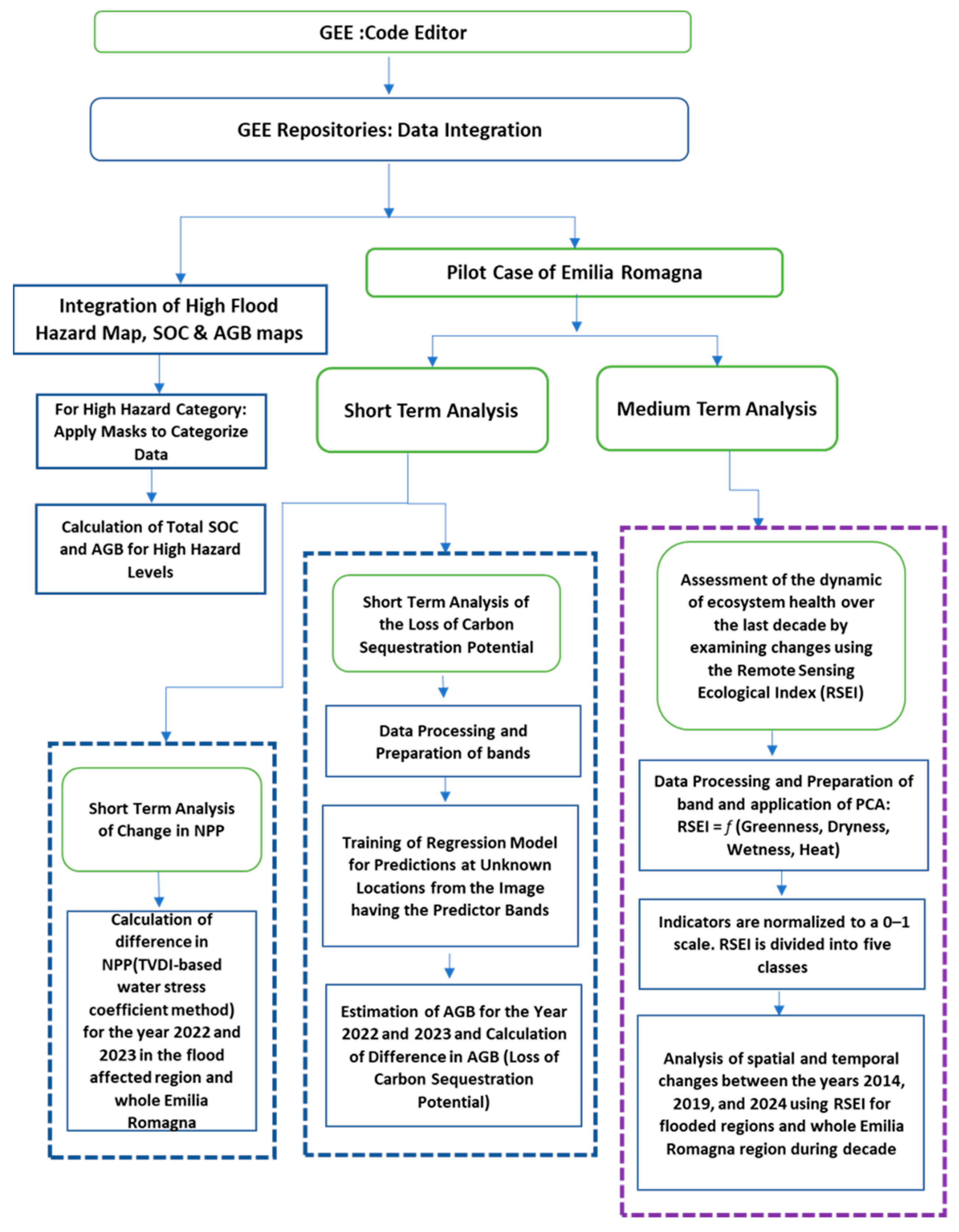
Figure 1. Schemataic flow chart of the methodology.
Water 17 03001 g001
Figure 2. Flood-affected region (FL23) for the year 2023 (flood polygons).
Water 17 03001 g002
Figure 3. NPP changes from 2022 to 2023.
Water 17 03001 g003
Figure 4. AGBD changes between 2022 and 2023.
Water 17 03001 g004
Figure 5. RSEI for the years 2014, 2019, and 2024.
Water 17 03001 g005
Figure 6. RSEI class distribution in (%) for the whole region of Emilia-Romagna and the flood-affected region.
Water 17 03001 g006
Figure 7. RSEI class transition (%) between 2014 and 2024 for the whole of Emilia-Romagna region and flood-affected region.
Water 17 03001 g007
Figure 8. High flood-hazard zone of the Emilia-Romagna region (as per Idrogeo).
Water 17 03001 g008
Figure 9. SOC at risk in high flood-risk region of Emilia-Romagna.
Water 17 03001 g009
Figure 10. AGBD at risk in high flood-risk region of Emilia-Romagna.
Water 17 03001 g010
Table 1. Indicators definition and implications.
Name of IndicatorDefinitionEcological Meaning of Its Changes
AGB (Above-Ground Biomass)Total mass of living plant material above the soil surface, typically measured in tons per hectare, derived from satellite data using vegetation indices.Decrease indicates vegetation loss.
Increase implies vegetation regrowth, recovery.
NPP (Net Primary Productivity)The net amount of carbon captured by ecosystem (vegetation) after subtracting autotrophic respiration, derived from satellite-based models.Reduction implies reduced photosynthetic activity.
Increase signifies enhanced growth.
RSEI (Remote Sensing Ecological Index)Composite ecological indicator derived from NDVI, LST (land surface temperature), wetness, and NDBSI (Normalized Difference Build-up and Soil Index) to assess ecological quality.Decrease suggests ecosystem degradation, reduced vegetation cover, or soil exposure. Increase shows ecological restoration, vegetation recovery, and improved land surface conditions.
Table 4. Changes in the areas of whole Emilia-Romagna and flood-affected region and net changes in AGB and NPP.
Area (%) 2022–23
NPPAGB
PositiveNegativePositiveNegative
Flood-affected region48.0451.9650.649.4
Whole Emilia-Romagna54.544.528.0469.4
Total NPP (g C yr−1) 2022–23
GainLossNet Gain/Loss
Flood-affected region1.5 × 104−2.2 × 10⁴−7.0 × 10³
Whole Emilia-Romagna2.7 × 106−2.1 × 1066.7 × 105
Total AGB (Mg) 2022–23
GainLossNet Gain/Loss
Flood-affected region0.5 × 103−1.0 × 10³−0.5 × 10³
Whole Emilia-Romagna2.8 × 104−3.5 × 10⁵−3.3 × 10⁵
Table 5. Area belonging to ecological quality classes over the years.
YearPoor (0–0.2)Fair (0.2–0.4)Moderate (0.4–0.6)Good (0.6–0.8)Very Good (0.8–1.0)
Whole Region of Emilia-Romagna
2014846.3 km2 (3.8%)20,847.0 km2 (93.9%)197.9 km2 (0.9%)167.1 km2 (0.8%)35.6 km2 (0.5%)
20193112.1 km2 (14.0%)18,711.4 km2 (84.6%)93.8 km2 (0.04%)175.9 km2 (0.07%)0.8 km2 (0.0%)
202410,269.2 km2 (46.4%)11,547.7 km2 (52.2%)172.3 km2 (0.7%)104.9 km2 (0.4%)0.1 km2 (0.00%)
Flood-Affected Region of Emilia-Romagna
201417.0 km2 (5.3%)301.2 km2 (93.8%)2.7 km2 (0.8%)0.3 km2 (0.1%)0.1 km2 (0.00%)
201957.8 km2 (17.9%)262.2 km2 (81.6%)1.2 km2 (0.3%)0.1 km2 (0.00%)0.0 km2 (0%)
202496.0 km2 (29.8%)224.0 km2 (69.8%)1.0 km2 (0.3%)0.2 km2 (0.06%)0.0 km2 (0%)
Table 6. Ecological quality classes transition over a period (adopted from Yan. et al., 2021 [41]): area in km2 and percentage of the total.
PeriodS–4S–3S–2S–1Stable (S0)S + 1S + 2S + 3S + 4
Whole Region of Emilia-Romagna
2014–190.0 (0.0%)0.3 (0.00%)6.4 (0.03%)2953
(13.7%)
18,624.9 km2 (84.3%)507.6 (2.3%)1.3
(0.01%)
0.04 (0.0002%)0.0 (0.0%)
2019–240.0 (0.0%)0.1
(0.0%)
2.6 (0.01%)8280 (37.48.0%)12,750.1 km2 (57.71%)1058.1 (4.79%)2.5
(0.01%)
0.0
(0.0%)
0.0 (0.0%)
2014–240.0 (0.0%)0.9
(0.0%)
22.6 (0.10%)9934 (44.96%)11,835.8 km2 (53.57%)299.7 (1.3%)1.2
(0.01%)
0.01 (0.0004%)0.0 (0.0%)
Flood-Affected Region of Emilia-Romagna
PeriodS–4S–3S–2S–1Stable (s0)S + 1S + 2S + 3S + 4
2014–190.0 (0.0%)0.03 (0.01%)0.13 (0.04%)47.3 (16.63%)227.1 km2 (79.60%)10.4 (3.64%)0.01 (0.004%)0.0
(0.0%)
0.0 (0.0%)
2019–240.0 (0.0%)0.00 (0.0%)0.01 (0.0%)65.7 (23.05%)188.4 km2 (66.11%)30.8 (10.8%)0.07 (0.02%)0.0
(0.0%)
0.0 (0.0%)
2014–240.0 (0.0%)0.02 (0.0%)0.13 (0.05%)79.9 (28.04%)196.7 km2 (69.03%)8.17 (2.86%)0.01 (0.004%)0.0
(0.0%)
0.0 (0.0%)
Notes: Change level included S+ 4, S + 3, S + 2, S + 1, S (0), S−1, S−2, S−3, and S−4. + 4, +3, +2, and +1 represents ecological improvement levels 4, 3, 2, and 1, respectively. S (0) represents no change in ecological level and −1, −2, −3, and −4 represents successive degrees of degradation.
Table 7. Estimated carbon stocks (total SOC and total AGB) in high-hazard flood-prone areas.
Carbon StocksQuantity Estimated in High-Hazard-Prone Area
SOC1.1 × 107 Mg C
AGB9.0 × 106 Mg C
Disclaimer/Publisher’s Note: The statements, opinions and data contained in all publications are solely those of the individual author(s) and contributor(s) and not of MDPI and/or the editor(s). MDPI and/or the editor(s) disclaim responsibility for any injury to people or property resulting from any ideas, methods, instructions or products referred to in the content.