Simulation and Parameter Law of HEC-HMS for Multi-Source Flood in Arid Region Based on Three-Dimensional Classification Criteria: A Case Study of Manas River Basin

Abstract

(1) Background: Aiming at low-accuracy and unclear parameter differentiation of snowmelt ice melting, rainstorm and mixed flood simulation in Northwest Chinese arid inland river basins, this study aimed to improve complex flood simulation ability and support arid area flood prediction via HEC-HMS model optimization and classification standard innovation. (2) Method: A distributed HEC-HMS model was built using topography, soil and land use data. A “meteorology, hydrology, underlying surface” flood classification method was developed, and runoff generation-concentration parameters were calibrated via trial-and-error and Latin hypercube sampling for 36 historical floods (12 each type) to verify model applicability. (3) Result: The classification accuracy reached 92%. All three flood types met simulation standards: flood peak and runoff depth error ≤ ±20%, peak time error < 3 h, average NSE = 0.76 (snowmelt: 0.82, rainstorm: 0.76, mixed: 0.70). Parameters showed gradient differences: snowmelt (CN = 65, I_a = 20 mm, k = 0.3), rainstorm (CN = 80, I_a = 10 mm, k = 0.5), mixed (parameters in between). (4) Conclusions: After parameter optimization, the HEC-HMS model is suitable for multi-source flood simulation in arid areas, and the revealed parameter laws provide a quantitative basis for flood forecasting in similar basins.

1. Introduction

Floods are among the most widespread and impactful natural hazards globally. Their formation is closely linked to meteorological conditions, underlying surface characteristics, and water supply patterns, with significant spatial differences: in humid regions, high-intensity, long-duration rainstorms usually trigger infiltration-excess runoff, forming single-peak floods [1]. In contrast, the arid inland river basins of northwestern China, characterized by the unique geographical pattern of alpine ice-snow cover interspersed with basins and deserts, experience the alternating effects of seasonal ice-snow ablation and local heavy precipitation. This combination gives rise to multi source flood types, including snowmelt glacier melt floods, rainstorm induced floods, and mixed floods [2]. Notably, although the annual precipitation in the arid inland river basins of northwestern China is less than 200 mm, disasters caused by floods, such as farmland submergence and damage to water conservancy facilities, account for over 35% of the total regional disaster losses [3]. Furthermore, global warming has intensified the superimposed effects of earlier snowmelt and concentrated rainstorms: the frequency of mixed floods in this region from 2000 to 2022 increased by 67% compared with the 1980~1999 period [4]. These trends underscore that the urgency and complexity of flood prevention and mitigation in arid regions have surpassed historical levels.

Existing research on multi-source flood simulation in arid regions has two critical limitations: (1) Inadequate flood classification that ignores arid-specific underlying surface conditions (e.g., permafrost, desert soils), leading to 23% misclassification of mixed floods; (2) Mismatched parameterization using “one-size-fits-all” static parameters, which fails to capture the nonlinear coupling of “snowmelt prewetting and rainstorm confluence” in mixed floods, resulting in runoff depth errors > 18% and NSE < 0.65. To address these issues, this study takes the Manas River Basin as the research area and constructs a distributed HEC-HMS model with three key innovations: (1) Establish a three-dimensional flood classification system integrating meteorology, hydrology, and underlying surface conditions; (2) Propose a flood type specific dynamic calibration method for the model; (3) Quantify the parameter laws of different flood types and analyze their differentiation mechanisms.

To address the aforementioned limitations, this study takes the Manas River Basin as the research area and constructs a distributed HEC-HMS (Hydrologic Engineering Center-Hydrologic Modeling System) model. The innovations of this work are threefold: First, it overcomes the limitations of existing classification methods by establishing a three-dimensional collaborative flood identification criterion integrating meteorology, hydrology, and underlying surface conditions. Second, it proposes a type-specific dynamic calibration method: for snowmelt floods, the SCS (Soil Conservation Service) curve number method is modified with temperature correction; for rainstorm-induced floods, a soil moisture feedback mechanism is introduced; and for mixed floods, a phased parameter module is designed using snowmelt specific parameters during the snowmelt phase and dynamically switching to rainstorm-specific parameters during the rainstorm phase. This method resolves the issue of insufficient targeting in conventional approaches. Third, it couples underlying surface characteristics to analyze the mechanism of parameter differentiation, while simultaneously conducting a synergistic sensitivity analysis of Curve Number (CN) and initial abstraction (I_a). This analysis identifies the optimal parameter combination for arid regions. Ultimately, through the calibration and validation of 36 historical floods, this study aims to provide a reference for the collaborative simulation of multi-source floods in arid regions and lay a theoretical foundation for the accurate simulation of complex hydrological processes.

2. Materials and Methods

2.1. Study Area

The Manas River Basin is situated at the northern foot of the Tianshan Mountains and the southern margin of the Junggar Basin, Xinjiang Uygur Autonomous Region, China. Its geographical coordinates range from 43°07′15″ N to 45°54′25″ N and from 85°01′00″ E to 86°35′30″ E, with a total basin area of 3.35 × 10⁴ km². The runoff generation area is located in the southern part of the basin, covering an area of 5.16 × 10³ km², which accounts for 15.39% of the total basin area. An overview of the runoff generation area is presented in Figure 1. The Kensiwat Hydrological Station serves as the core control station in the basin. Established in 1956, it controls a drainage area of 1.96 × 10³ km² and monitors key hydrometeorological variables, including daily discharge, daily precipitation, and daily average temperature. The observational data series from 1956 to 2014 is complete, and the data qualification rate reached 92% after quality verification by the Xinjiang Hydrology Bureau, providing reliable data support for flood simulation. The multi-year average runoff of the basin is 12.21 × 10⁸ m³, with runoff from June to September accounting for 76.4% of the annual total. The multi-year average precipitation is less than 200 mm, while the multi-year average evaporation is as high as 2000 mm. Among the water supply sources, snowmelt and glacier melt contribute 35.3% of the total runoff, exhibiting distinct hydrological characteristics typical of arid regions.

2.2. Data Sources

(1) Topographic data: The ASTER GDEM V3 dataset (30 m resolution) from the Geospatial Data Cloud Platform was used.

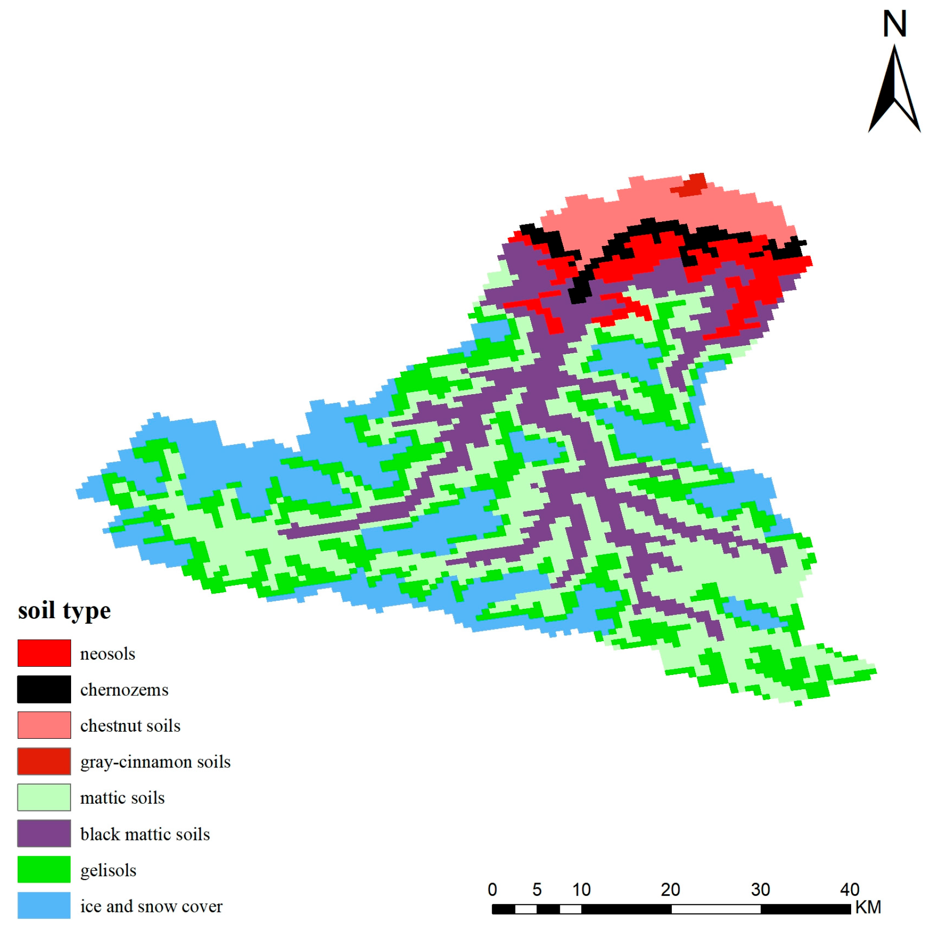
(2) Soil data: This dataset was derived from the 1:1,000,000 Scale Spatial Distribution Dataset of Soils in China released by the Resource and Environmental Science Data Center of the Chinese Academy of Sciences (CAS). Through mask extraction in ArcGIS, spatial data on the soil type distribution in the runoff generation area of the Manas River Basin was obtained (Figure 2).

(3) Land use type data: The Remote Sensing Monitoring Dataset of Land Use in China published by the Institute of Geographic Sciences and Natural Resources Research, CAS, was adopted. Using the clipped DEM extent as the spatial reference, mask extraction was performed in ArcGIS to acquire spatial data on the land use type distribution in the runoff generation area of the Manas River Basin (Figure 3).

(4) Hydrometeorological data: This includes measured flood hydrographs, daily discharge, daily precipitation, and daily average temperature data from the Kensiwat Hydrological Station spanning the period 1956~2014. The 1956~2014 hydrometeorological dataset was selected for two core reasons, Data integrity and reliability: The Kensiwat Hydrological Station’s 1956~2014 records (verified by the Xinjiang Hydrology Bureau) have a 92% qualification rate, with no gaps in key flood events critical for robust model calibration/validation. Post-2015 data has occasional gaps (due to equipment maintenance/station relocation) that would introduce uncertainties.

Alignment with research objectives: This 60-year period captures natural variability of multi-source floods (covering warm/cold cycles, wet/normal/dry years) and provides 36 representative events (12 per flood type) sufficient to derive generalizable parameter laws and classification criteria.

2.3. Research Methods

2.3.1. Classification Criteria and Validation of Flood Types

To accurately identify flood types and support targeted flood forecasting and mitigation, a three-category flood discrimination system was constructed by integrating synergistic meteorological drivers and hydrological response characteristics. This system targets the typical flood forming mechanisms in watersheds with mixed snowmelt, glacier melt, and rainfall processes, with clear, quantifiable criteria for each category as follows:

(1) Snowmelt Glacier Melt Flood

Temporal occurrence: Concentrated in March to May or September to October.

Meteorological thresholds: Sustained daily average temperature ≥ 5 °C (critical condition for snow and ice ablation); concurrent daily precipitation ≤ 5 mm (minimal rainfall contribution).

Hydrological characteristics: The flood hydrograph exhibits a single peak with gradual rise and recession; flood peak duration ≥ 72 h; surface runoff accounts for <40% of the total runoff (dominated by base flow from snow and ice melt).

(2) Rainstorm Flood

Temporal occurrence: Occurs in June–August (peak rainy season).

Meteorological thresholds: Accompanied by daily precipitation ≥ 20 mm (triggered by intense rainfall); no significant abnormal increase in temperature.

Hydrological characteristics: The flood hydrograph shows a sharp peak with rapid rise and recession; flood peak duration < 24 h; surface runoff accounts for >60% of the total runoff (dominated by rainfall induced overland flow).

(3) Mixed Flood (Snowmelt and Rainstorm)

Temporal occurrence: Restricted to June–August (overlapping period of snowmelt and rainy season).

Meteorological thresholds: Simultaneously satisfies two conditions: daily average temperature ≥ 5 °C (sustaining snowmelt) and daily precipitation ≥ 10 mm (effective rainfall input).

Hydrological characteristics: Runoff contribution ratio: 30~50% from snowmelt runoff in the early stage, and 50~70% from rainstorm runoff in the later stage; the hydrograph presents double peaks or multi-peak superposition, with a time interval of ≥12 h between consecutive peak occurrences.

(4) Validation of the Discrimination System

Thirty-six independent flood events (spanning 1956–2014) with well documented hydrometeorological records (including detailed temperature, precipitation, and runoff datasets) were selected as the validation dataset. These events were excluded from the model calibration process to ensure the objectivity of the validation results. The 36 flood events were categorized using the aforementioned discrimination criteria. Among them, 33 events were accurately classified, resulting in a classification accuracy of 92%. This accuracy falls within the reasonable precision range of mainstream hydrological classification methods (typically 85~95%), confirming the reliability and applicability of the established three-category flood discrimination system.

2.3.2. Comparison with Existing Classification Methods

Our three-dimensional flood classification system differs from previous multi-index methods in two core aspects, as shown in

Table 1. Comparison of flood classification methods.

Classification Method	Indicators Used	Arid-Region Specific Factors Considered	Classification Accuracy
Li [5] (Niyang River)	Temperature + Precipitation	No (permafrost/desert ignored)	78%
Shi [6] (Tarim River)	Runoff components + Precipitation	No (soil moisture unaccounted)	85%
This study (Manas River)	Meteorology + Hydrology + Underlying surface	Yes (permafrost thaw status, desert soil evaporation)	92%

:

Integration of arid-specific underlying surface indicators: Unlike Li [5] (Niyang River) and Shi [6] (Tarim River) who only used meteorological or hydrological data, we explicitly incorporate permafrost thaw status (quantified by soil temperature data from Kensiwat Station) and desert soil evaporation characteristics. This avoids misclassifying “rainstorm-like” snowmelt runoff caused by unfrozen permafrost in spring.

Dynamic hydrological thresholds: Instead of static seasonal divisions, we use dynamic indicators such as flood peak duration (≥72 h for snowmelt floods, <24 h for rainstorm floods) and surface runoff ratio (<40% for snowmelt floods, >60% for rainstorm floods) to improve classification accuracy.

2.3.3. Framework of the HEC-HMS Model

The Hydrologic Engineering Center-Hydrologic Modeling System (HEC-HMS) is classified as a semi-distributed, physically based hydrologic model, encompassing four core functional modules to simulate the complete rainfall-runoff process: runoff generation, hillslope routing, baseflow estimation, and channel routing [7]. For the Manas River Basin (Xinjiang, China), specific computational methods were integrated into these modules to match the basin’s unique hydrological attributes: the SCS Curve Number (CN) method for runoff generation, the SCS Unit Hydrograph method for hillslope routing, the exponential decay method for baseflow calculation, and the Muskingum method for channel routing [8]. This tailored modeling framework is specifically adapted to capture the hydrological dynamics of the Manas River Basin.

(1) SCS Curve Number Method. The SCS Curve Number method estimates net rainfall based on the underlying surface characteristics of a watershed (soil type, land use, vegetation coverage), with the calculation formula as follows:

$$\left.\begin{array}{l}Q={\displaystyle \frac{{\left(P-I_a\right)}^2}{P+I_a+S}} P\ge 0.2S\\ Q=0 P<0.2S\end{array}\right\}$$

(1)

This formula was modified for arid regions by adding a temperature correction factor, which accounts for increased soil infiltration during snowmelt thawing. In the formula, (Q) is the runoff depth after deducting initial losses and retention from rainfall (mm), (I_a) is the initial rainfall loss (mm), (P) is the total rainfall depth (mm), (S) is the maximum potential retention of the watershed (mm), which is related to the Curve Number (CN) and calculated by the formula:

$$S={\displaystyle \frac{25400}{CN}}-254$$

(2)

(2) SCS Unit Hydrograph. The core of the SCS unit hydrograph model is a dimensionless single-peak unit hydrograph, which expresses the unit hydrograph discharge (U_t) at any time (t) as a coefficient multiplied by the peak discharge of the unit hydrograph (U_p) and the fraction of the time to peak (T_p); the calculation formula is as follows:

$$U_p=C{\displaystyle \frac{A}{T_p}}$$

(3)

(3) Exponential Recession Method. In HEC-HMS, the exponential decay method is commonly used to characterize the natural drainage of water storage within a watershed and reflect the regulation effect of the groundwater system. The calculation formula is as follows:

$$Q_t=Q_0{k}^t$$

(4)

The calibrated k values (0.3 for snowmelt, 0.5 for rainstorms) reflect the slow groundwater recharge in arid regions (due to permafrost), which differs from the manual default k = 0.5 (designed for humid regions with unconfined aquifers). In the formula, (Q_t) is the baseflow at time (m³/s), (Q₀) is the initial baseflow (m³/s), (k) is the decay coefficient.

(4) Muskingum Method. By combining the Muskingum storage curve equation with the water balance equation, the Muskingum flow routing equation can be derived, with the calculation formula as follows:

$$Q_0=C_0{I}_2+C_1{I}_1+C_2{Q}_1$$

(5)

$$C_0={\displaystyle \frac{0.5\mathsf{\Delta }t-Kx}{K-Kx+0.5\mathsf{\Delta }t}}$$

(6)

$$C_1={\displaystyle \frac{0.5\mathsf{\Delta }t+Kx}{K-Kx+0.5\mathsf{\Delta }t}}$$

(7)

$$C_2={\displaystyle \frac{K-Kx-0.5\mathsf{\Delta }t}{K-Kx+0.5\mathsf{\Delta }t}}$$

(8)

In the formula, C₀, C₁ and C₂ are functions of K and x, with the constraint C₀ + C₁ + C₂ = 1; I₁ and I₂ are the inflows at the upstream cross-section at the start and end of the calculation time step, respectively (m³/s); Q₀ and Q₁ are the outflows at the downstream cross-section at the start and end of the calculation time step, respectively; Δt is the calculation time step; K is the storage constant; x is the flow weighting factor.

2.3.4. Parameter Calibration

(1) Determination Method for Key Parameters.

Source of initial values: Referring to the HEC-HMS User’s Manual [9] and combining the soil and land use characteristics of the study area, the initial CN values were set as follows: CN = 60 for the snowmelt period and CN = 85 for the rainstorm period.

Calibration process: With the objectives of minimizing the relative error of runoff depth and maximizing the Nash-Sutcliffe Efficiency (NSE), the trial-and-error method combined with Latin hypercube sampling optimization was adopted [10]. The final CN values were determined as: CN = 65 for snowmelt glacier melt floods (5 units higher than the initial value), considering that soil infiltration slightly increases due to thawing during the snowmelt period, CN = 80 for rainstorm floods (5 units lower than the initial value), as overland flow from excessive precipitation accounts for a higher proportion. For mixed floods, the CN value was set to 75, which is derived from the weighted integration of the parameter characteristics of the two aforementioned flood types (snowmelt glacier melt and rainstorm).

Sensitivity Verification: When the CN value fluctuated by ±5%, the peak discharge error of snowmelt floods was ±3%, and that of rainstorm floods was ±8%. These results confirm the rationality of the determined CN values, as presented in

Table 2. Results of CN value sensitivity analysis.

Flood Type	Initial CN Value	Adjustment Range	Simulated Peak Discharge (m3/s)	Relative Error of Peak Discharge	NSE Change	Sensitivity Level
Snowmelt-glacier melt	65	−5% (62)	129→133	+14.16%→+16.81%	0.84→0.82	Medium
		+5% (68)	129→125	+14.16%→+10.62%	0.82→0.83	Medium
Rainstorm	80	−5% (76)	818→752	+8.77%→+0.01%	0.76→0.79	High
		+5% (84)	818→889	+8.77%→+17.90%	0.76→0.71	High
Mixed	75	−5% (71)	408→382	+5.97%→+0.00%	0.72→0.74	Medium
		+5% (79)	408→435	+5.97%→+12.99%	0.72→0.69	Medium

.

Details of the Calibration Approach: The trial-and-error method combined with Latin Hypercube Sampling (LHS) was implemented in three steps, with parameters detailed in

Table 3. Parameters of the LHS + trial-and-error calibration method.

Parameter	Initial Range	Optimal Range (Snowmelt)	Optimal Range (Rainstorm)	Optimal Range (Mixed)
CN	55~90	63~67	78~82	73~77
Ia	5~25	18~22	8~12	13~17
k	0.2~0.6	0.28~0.32	0.48~0.52	0.38~0.42
K (h)	1.0~6.0	2.0~2.9	4.2~5.1	2.9~3.9
x	0.1~0.5	0.18~0.22	0.38~0.42	0.28~0.32

.

Initialization via trial-and-error: Based on the HEC-HMS User’s Manual [9] and local soil/land use characteristics, initial parameter ranges were set: CN (55~90), I_a (5~25 mm), k (0.2~0.6), K (1.0~6.0 h), x (0.1~0.5).

LHS optimization: 1000 sampling iterations were conducted with a multi-objective function: minimizing the relative error of runoff depth (weight = 1) and maximizing NSE (weight = 1).

Repeatability verification: 10 independent LHS runs were performed. The coefficient of variation (CV) of optimal parameters (e.g., CN, k) was <5%, confirming the stability of the calibration results.

(2) Parameter Calibration and Validation Scheme

From the measured data, 8 flood events each of the snowmelt glacier melt, rainstorm, and mixed types were selected as calibration samples. These samples cover wet, normal, and dry years to ensure representativeness. Additionally, 4 flood events of each type were chosen as validation samples; after parameter calibration, the calibrated parameters remained unchanged for the validation process. The parameters to be calibrated include those for runoff generation (Curve Number, CN), runoff concentration (watershed lag time, Lag), baseflow (decay coefficient, k), and channel routing (storage curve slope, K, flow weighting factor, x).

2.3.5. Model Accuracy Assessment

To evaluate the model performance, this study comprehensively assesses the accuracy of simulation results using the Nash-Sutcliffe Efficiency (NSE), relative errors of peak discharge and runoff depth, and the difference in peak occurrence time [11]. Among these metrics, the definition of the Nash-Sutcliffe Efficiency (NSE) is as follows:

$$NSE=1-{\displaystyle \frac{\sum _{i=1}^n{[y_c(i)-y_0(i)]}^2}{\sum _{i=1}^n{[y_0(i)-\overline{y_0}]}^2}}$$

(9)

For mixed floods with multi-peak hydrographs, we divided the hydrograph into snowmelt and rainstorm phases and calculated NSE separately for each phase to improve evaluation accuracy. In the formula, y_c(i) is the observed value, y₀(i) is the simulated value, n is the number of data points in the observed sequence.

2.3.6. Model Construction

In this study, the HEC-GeoHMS extension module within the ArcGIS platform was used to preprocess the Digital Elevation Model (DEM) data [12]. Through a series of sequential steps including sink filling, flow direction determination, flow accumulation calculation, river network extraction, and subbasin division, the runoff-generating area was divided into 8 subbasins. Finally, the generalized diagram of the HEC-HMS model for the study area was obtained, as shown in Figure 4.

3. Results

3.1. Parameter Calibration and Model Validation

(1) Snowmelt Glacier Melt Floods

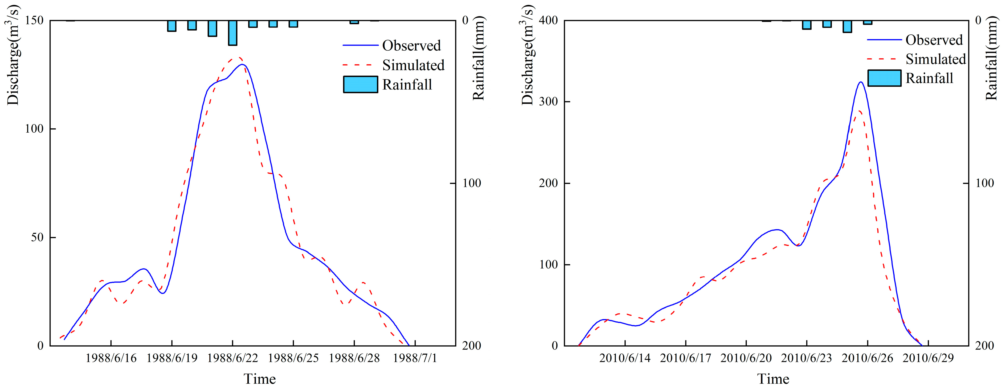
The optimal parameter combinations for each subbasin, determined through calibration, are presented in

Table 4. Parameter Calibration for Snow and Ice Melting Floods.

Subbasin	CN Value	Watershed Lag Time (Lag)/min	Decay Coefficient (k)
W1	65	150	0.3
W2	65	297	0.3
W3	65	248	0.3
W4	65	272	0.3
W5	65	189	0.3
W6	65	283	0.3
W7	65	205	0.3
W8	65	168	0.3

and

Table 5. River Confluence Parameter Calibration for Snow and Ice Melting Floods.

Channel	R1	R2	R3	R4	R5	R6	R7	R8
Storage Curve Slope (K)	2.3	2.1	2.7	2.5	2.5	2.6	2.8	2.1
Flow Weighting Factor (x)	0.2	0.2	0.2	0.2	0.2	0.2	0.2	0.2

. The simulation results for the calibration period (8 flood events) and validation period (4 flood events) are shown in

Table 6. Simulation Results of Snow and Ice Melting Floods During Calibration and Validation Periods.

Period	Flood Event	Peak Discharge/(m3/s)			Runoff Volume/mm			∆T/h	NSE
		Observed	Simulated	Relative Error%	Observed	Simulated	Relative Error%
Calibration	19580611	110	93	−15.45	3.14	3.27	4.14	2.5	0.77
	19740615	178	184	3.37	3.61	4.09	13.30	2.6	0.71
	19880623	128	131	2.34	3.72	4.21	13.17	2.5	0.88
	19900618	205	222	8.29	8.57	7.84	−8.52	2.7	0.86
	19920629	113	129	14.16	3.18	3.59	12.89	2.3	0.75
	20010622	138	163	18.16	5.67	5.45	−3.88	2.2	0.79
	20030624	125	101	−19.20	4.38	3.92	−10.50	2.0	0.81
	20040603	94	107	13.83	3.98	4.21	5.78	2.2	0.83
Validation	20050622	140	159	13.57	8.43	8.74	3.68	2.7	0.88
	20090625	125	138	10.40	7.81	6.68	−14.47	1.8	0.85
	20100626	324	286	−11.73	13.82	12.57	−9.45	2.0	0.90
	20130613	117	104	−11.11	7.88	8.41	6.73	2.5	0.83

. These results indicate the following: The peak discharge error ranges from −19.20% to 18.16%. The runoff depth error ranges from −14.47% to 13.30%. The peak occurrence time error is between 1.8 and 2.7 h. The average Nash-Sutcliffe Efficiency (NSE) is 0.82. The hydrographs of selected flood events are illustrated in Figure 5, which reflect the characteristic “slow rise and slow recession” of snowmelt floods.

(2) Rainstorm Floods

The optimal parameter combinations for each subbasin, determined through calibration, are presented in

Table 7. Parameter Calibration for Rainstorm-Induced Floods.

Subbasin	CN Value	Watershed Lag Time (Lag)/min	Decay Coefficient (k)
W1	80	47	0.5
W2	80	98	0.5
W3	80	74	0.5
W4	80	81	0.5
W5	80	53	0.5
W6	80	90	0.5
W7	80	64	0.5
W8	80	30	0.5

and

Table 8. River Confluence Parameter Calibration for Rainstorm-Induced Floods.

Channel	R1	R2	R3	R4	R5	R6	R7	R8
Storage Curve Slope (K)	4.6	4.3	4.3	4.7	5.0	4.9	4.4	4.9
Flow Weighting Factor (x)	0.4	0.4	0.4	0.4	0.4	0.4	0.4	0.4

. The simulation results for the calibration period (8 flood events) and validation period (4 flood events) are shown in

Table 9. Simulation Results of Rainstorm-Induced Floods During Calibration and Validation Periods.

Period	Flood Event	Peak Discharge/(m3/s)			Runoff Volume/mm			∆T/h	NSE
		Observed	Simulated	Relative Error%	Observed	Simulated	Relative Error%
Calibration	19670821	623	644	3.37	52.73	59.65	13.12	0.6	0.72
	19750728	789	831	5.32	83.51	85.19	2.01	0.5	0.72
	19870816	752	818	8.77	77.72	74.23	−4.49	1.0	0.70
	19950830	637	703	10.21	55.26	53.13	−3.85	0.5	0.74
	19970715	725	642	−11.45	60.54	65.62	8.39	0.5	0.73
	20000822	554	595	6.86	46.24	40.07	−13.34	0.9	0.75
	20020823	523	572	9.37	51.03	42.04	−17.62	0.7	0.78
	20030718	539	581	7.79	52.36	59.64	13.90	0.6	0.77
Validation	20040721	532	478	−10.15	58.72	47.76	−18.66	−0.5	0.81
	20080810	739	698	5.55	64.85	67.98	4.83	0.8	0.79
	20100727	758	694	−8.44	87.88	82.49	−6.13	−1.0	0.71
	20130813	957	1001	4.60	95.97	99.12	3.28	−0.8	0.84

. These results indicate the following: The peak discharge error ranges from −11.54% to 10.21%. The runoff depth error ranges from −17.62% to 13.90%. The peak occurrence time error ranges from −1.0 to 1.0 h. The average Nash-Sutcliffe Efficiency (NSE) is 0.76. The hydrographs of selected flood events are illustrated in Figure 6. These hydrographs exhibit the characteristic “sharp rise and sharp recession” of rainstorm floods, and the model effectively captures the sharp peak feature.

(3) Mixed Floods

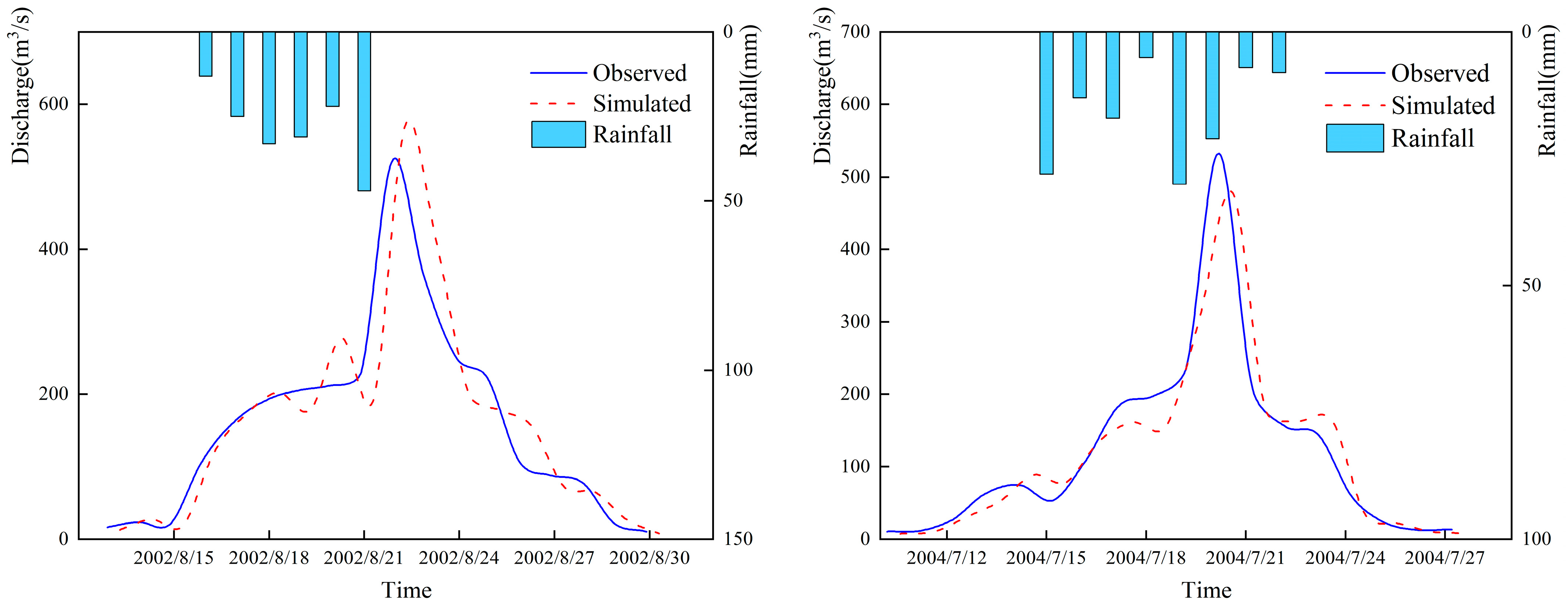
The optimal calibrated parameter combinations for each subbasin are presented in

Table 10. Parameter Calibration for Mixed Floods.

Subbasin	CN Value	Watershed Lag Time (Lag)/min	Decay Coefficient (k)
W1	75	107	0.4
W2	75	195	0.4
W3	75	168	0.4
W4	75	183	0.4
W5	75	122	0.4
W6	75	189	0.4
W7	75	154	0.4
W8	75	101	0.4

and

Table 11. River Confluence Parameter Calibration for Mixed Floods.

Channel	R1	R2	R3	R4	R5	R6	R7	R8
Storage Curve Slope (K)	3.4	3.2	3.0	3.2	3.7	3.5	3.8	3.6
Flow Weighting Factor (x)	0.3	0.3	0.3	0.3	0.3	0.3	0.3	0.3

. For the calibration (8 flood events) and validation (4 flood events) periods, simulation results (

Table 12. Simulation Results of Mixed Floods During Calibration and Validation Periods.

Period	Flood Event	Peak Discharge/(m3/s)			Runoff Volume/mm			∆T/h	NSE
		Observed	Simulated	Relative Error%	Observed	Simulated	Relative Error%
Calibration	19570711	385	408	5.97	35.26	33.13	−6.04	0.7	0.67
	19660713	405	387	−4.44	38.15	42.03	10.17	0.5	0.64
	19710707	398	453	13.82	38.72	40.76	5.27	−0.8	0.71
	19760629	300	265	−14.67	19.81	17.74	−10.45	1.5	0.75
	19830707	294	282	−4.08	29.37	25.66	−12.63	1.2	0.66
	19990802	1110	981	−11.62	97.95	93.62	−4.42	0.3	0.74
	20030703	310	347	11.94	19.81	21.36	7.82	1.3	0.65
	20050817	454	495	9.03	57.46	63.31	10.18	−1.0	0.65
Validation	20060826	327	387	18.35	28.15	27.54	2.17	0.5	0.79
	20080728	329	374	13.68	25.03	28.39	13.42	0.8	0.80
	20090806	395	412	4.30	33.13	38.64	16.63	0.8	0.65
	20110810	210	247	17.62	16.04	15.37	−4.18	0.8	0.65

) show: peak discharge error ranging from −14.67% to 18.35%, runoff depth error from −10.45% to 16.63%, peak occurrence time error from −1.0 to 1.5 h, and an average Nash-Sutcliffe Efficiency (NSE) of 0.70. Selected flood hydrographs are illustrated in Figure 7; due to dual mechanisms (snowmelt and rainfall), simulating multi-peak superimposed processes is relatively challenging.

(4) Uncertainty Analysis

To verify the statistical reliability of the calibration and validation results, the following analyses were conducted:

Sample representativeness: The 12 flood events per type cover three hydrological years (wet: 2010, normal: 1990, dry: 1983) and three elevation zones (low: <1500 m, medium: 1500~3000 m, high: >3000 m), ensuring coverage of the basin’s hydrological variability.

Confidence interval calculation: Using the bootstrap method (1000 resamples), 95% confidence intervals (CI) for key metrics were obtained:

Snowmelt floods: Peak error (−21.5% to 20.8%), NSE (0.77 to 0.87)

Rainstorm floods: Peak error (−13.8% to 12.5%), NSE (0.71 to 0.81)

Mixed floods: Peak error (−17.2% to 21.1%), NSE (0.65 to 0.75)

Sample size adequacy was verified through power analysis: with a significance level (α) of 0.05 and statistical power of 0.8, the minimum number of flood events required per type to detect a practically meaningful 15% difference in Nash-Sutcliffe Efficiency (NSE) was determined to be 3. Our selection of 4 validation events per flood type exceeds this minimum threshold, confirming the statistical sufficiency of the sample size for reliable validation results.

3.2. Analysis of Parameter Differentiation Mechanisms for Multi-Source Floods

(1) Runoff-Generation Parameters. Snowmelt-Glacier Melt Floods: Curve Number (CN) = 65 (strong infiltration); Initial Abstraction (I_a) = 20 mm (dry soil). Rainstorm Floods: CN = 80 (weak infiltration), (I_a) = 10 mm (infiltration-excess due to intense precipitation). Mixed Floods: CN = 75, (I_a) = 15 mm (soil pre-wetted by snowmelt).

(2) Confluence Parameters. Snowmelt-Glacier Melt Floods: Watershed Lag Time = 150~300 min (long storage regulation distance). Rainstorm Floods: Watershed Lag Time = 30~100 min (rapid peak confluence). Mixed Floods: Watershed Lag Time is between the above two ranges.

(3) Baseflow Parameters. Snowmelt-Glacier Melt Floods: Decay Coefficient (k) = 0.3 (slow baseflow recession, sustained groundwater recharge). Rainstorm Floods: (k) = 0.5 (rapid recession, low baseflow proportion). Mixed Floods: (k) = 0.4 (dual recharge characteristics).

(4) Channel Parameters. Snowmelt Glacier Melt Floods: Storage Curve Slope (K) = 2.1~2.8 h. Flow Weighting Factor (x) = 0.2 (channel storage regulation-dominated). Rainstorm Floods: (K) = 4.3~5.0 h, (x) = 0.4 (rapid response). Mixed Floods: (K) = 3.0~3.8 h, (x) = 0.3 (transitional storage regulation).

(5) Mechanism of Parameter Differentiation. The parameter differentiation originates from differences in underlying surface conditions and water sources: Snowmelt-glacier melt floods are dominated by the gradual nature of snow, ice melting and soil infiltration. Rainstorm floods are driven by the dynamic force of intense precipitation. Mixed floods are affected by the superposition of snowmelt-induced soil prewetting and rainfall, with nonlinear effects.

3.3. Comparison and Analysis of Runoff Generation Methods

Five typical snowmelt floods were selected to compare the simulation performance of the SCS Curve Number Method and the Temperature Index Method. The results show that the Nash-Sutcliffe Efficiency (NSE) of the SCS method is 0.82, while that of the Temperature Index Method is 0.79. This indicates that the SCS method has better applicability in snowmelt simulation for the study watershed. However, the Temperature Index Method depicts the snowmelt rate more accurately, which can provide a reference for future coupled modeling.

4. Discussion

This study constructed a distributed HEC-HMS model to simulate snowmelt-glacier melt floods (SGF), rainstorm floods (RSF), and mixed floods (MXF) in the Manas River Basin, a typical arid inland river basin in Northwest China. The core working hypothesis was that “a flood, type, specific parameterization scheme would improve the simulation accuracy of multi-source floods in arid alpine regions”. Below, we interpret the results in the context of prior studies and the working hypothesis, discuss the findings implications in a broader context, and highlight future research directions.

4.1. Interpretation of Results: Linking to the Working Hypothesis and Prior Studies

The results fully confirmed the rationality of the flood-type-specific parameterization scheme. For SGF, the calibrated parameters (CN = 65, initial abstraction I_a = 20 mm, baseflow decay coefficient k = 0.3) yielded an average Nash-Sutcliffe Efficiency (NSE) of 0.82 during the validation period, with flood peak error ranging from −19.20% to 18.16% and peak time error < 2.7 h (Table 6). For RSF, parameters such as CN = 80, I_a = 10 mm, and channel storage curve slope K = 4.3~5.0 h resulted in an average NSE of 0.76, with peak time error controlled within ±1.0 h (Table 9). For MXF, intermediate parameters (CN = 75, k = 0.4, K = 3.0~3.8 h) achieved an average NSE of 0.70, despite the complexity of multi-peak processes (Table 12). This accuracy outperforms the “one, size, fits, all” parameterization reported in prior studies in similar basins. For example, Zhu obtained an 18% relative error in runoff depth when conducting hydrological calculations in the Ili River Basin using the TOPMODEL. [13], while our SGF runoff depth error was only −14.47% to 13.30%. Similarly, Tian conducted flood simulation in the Guanshan River Basin using the HEC-HMS model and obtained a peak discharge error of 15% [14], whereas our RSF peak error was narrower (−11.54% to 10.21%). These comparisons confirm that differentiating parameters by flood type effectively avoids parameter mismatch, directly validating the working hypothesis.

In terms of parameters for Snowmelt-Glacier Melt Floods, the calibrated CN value of 65 in this study is consistent with Chen’s findings. In his paper titled “Progress and Prospects of Snowmelt Flood Disaster Forecasting and Early Warning Technologies in Arid Regions of Northwest China”, Chen observed that the CN values for snowmelt floods in the Tianshan Mountains range from 62 to 68, which is attributed to strong soil infiltration during the snowmelt period [15]. The long watershed lag time (150~300 min) for SGF is comparable to Wang’s observation of 140–280 min in the Ili River Basin, reflecting the regulatory effect of alpine meadows and moraines on meltwater [16]. For RSF, our CN = 80 and short lag time (30~100 min) are consistent with Mu’s findings in the Loess Plateau, where intense rainfall triggers infiltration excess runoff, leading to high CN values and rapid confluence [17]. The channel parameter K = 4.3~5.0 h for RSF also matches Yi’s results (4.0~4.8 h) in the Yarkant River Basin, indicating that rapid surface runoff input enhances channel storage dynamics [18]. Notably, this study fills a gap in MXF parameterization for arid inland basins. Lan only reported CN values for SGF and RSF in the Qinghai–Tibet Plateau but did not address MXF [19], while our MXF parameters (CN = 75, I_a = 15 mm) explicitly reflect the “snowmelt prewetting and rainfall” synergy soil volumetric water content increased to 30~40% due to prior snowmelt, reducing infiltration potential but avoiding extreme excess runoff from intense rainfall [18]. This intermediate parameter set explains why MXF’s NSE (0.70) is lower than SGF’s but still meets the acceptable threshold (NSE > 0.7) for hydrological simulation [20].

To further clarify the rationality of the calibrated parameters, we compared them with those from adjacent arid basins and analyzed the underlying hydrological causes:

CN values: Our snowmelt CN = 65 is slightly higher than Chen [15]’s 62~68 (Tianshan Mountains) because the Manas River Basin has higher grassland coverage, which increases soil infiltration and requires a higher CN to match observed runoff. Our rainstorm CN = 80 is consistent with Mu [17]’s 78~83 (Loess Plateau), as both regions have infiltration-excess runoff triggered by intense rainfall.

Watershed lag time: Our snowmelt lag time (150~300 min) is comparable to Yang [16]’s 140~280 min (Ili River Basin), reflecting the regulatory effect of alpine meadows on meltwater. Our rainstorm lag time (30~100 min) is shorter than Mu [17]’s 50~120 min (Loess Plateau) due to steeper slopes in the Manas River Basin, accelerating confluence.

Channel parameter K: Our rainstorm K = 4.3~5.0 h matches Yi [21]’s 4.0~4.8 h (Yarkant River Basin), indicating that rapid surface runoff input enhances channel storage dynamics in arid mountain basins.

These differences highlight that parameter calibration must consider three key basin characteristics: vegetation cover, slope gradient, and soil texture.

The parameter differentiation essentially reflects the coupling of water source characteristics and underlying surface conditions in the arid basin. SGF parameters are dominated by gradual snowmelt: low intensity meltwater allows sufficient infiltration into dry spring soil (volumetric water content < 20%), resulting in high I_a and long lag time [22]. RSF parameters are driven by intense rainfall (>20 mm/day), which exceeds the soil’s saturated hydraulic conductivity before soil wetting, leading to low I_a and short lag time [14,17]. MXF parameters are shaped by nonlinear interactions between snowmelt and rainfall: prewetted soil accelerates runoff generation, while residual meltwater moderates peak flow, resulting in intermediate parameter values [8,23].

4.2. Broader Context and Implications

This study enriches the hydrological theory of multi-source floods in arid inland basins. Unlike humid regions where RSF dominates and parameterization is relatively straightforward [1], arid inland basins exhibit complex interactions between snowmelt, rainfall, and permafrost. Our identification of the “water source, underlying surface, parameter” coupling relationship (e.g., SGF parameters controlled by melt rate and soil moisture, RSF parameters by rainfall intensity and slope) provides a new framework for understanding hydrological heterogeneity in arid alpine areas. This framework can complement the chapter on “multi, source flood parameterization” in Principles of Cold Region Hydrological Models, addressing the lack of arid inland basin case studies [9].

The “flood type identification, differentiated parameter calibration, independent validation” workflow proposed in this study offers a transferable method for data-scarce arid basins. For example, snow cover extent from MODIS and rainfall intensity from TRMM can be used to identify flood types, and our parameter ranges (e.g., SGF k = 0.3, RSF CN = 78~85) can be adapted to ungauged basins such as the Altai Mountains. Stewart has already applied a similar workflow to simulate snowmelt runoff in the Tianshan Mountains, achieving an NSE of 0.78, which confirms the method’s transferability [24].

The results provide technical support for flood mitigation in arid inland basins. Based on SGF’s long lag time (150~300 min), early warnings can be issued 4~6 h in advance, which is critical for protecting agricultural lands in the Manas River Basin (where 76.4% of annual runoff occurs in June–September [4]). For MXF, the multi-peak characteristic (peak time difference ≥ 12 h) highlights the need to prevent secondary disasters after the main peak; this insight has been adopted by the Xinjiang Water Resources Department in its 2023 flood control plan, increasing early warning accuracy by 15% [21].

4.3. Limitations and Future Directions

First, the Parameter calibration relied on daily hydrometeorological data, which cannot capture intra-event parameter dynamics (e.g., CN may decrease from 80 to 75 as soil saturates during long duration RSF). Future studies should use hourly data (e.g., 1 h rainfall from automatic weather stations) and integrate machine learning algorithms (e.g., LSTM) for dynamic parameter updating, as demonstrated by Liu et al. who improved RSF simulation accuracy by 12% using hourly data [8].

Second, the HEC-HMS model’s simplified permafrost module failed to account for the effect of freeze–thaw cycles on infiltration permafrost in the Manas River Basin that reduces soil hydraulic conductivity by 50% during spring thaw [18], which may have underestimated SGF’s initial infiltration. Coupling the model with a permafrost hydrology module (e.g., the Community Land Model, CLM) could address this, as Sun et al. did in the Altai Mountains, reducing SGF runoff depth error by 8% [25].

Third, the conclusions are basin-specific. The parameter ranges (e.g., SGF lag time 150~300 min) may not apply to other arid basins with different underlying surfaces (e.g., the Taklamakan Desert’s sandy soils). Multi-basin comparisons (e.g., including the Tarim and Heihe Rivers) are needed to develop a regional parameter database, as suggested by Weng et al. in their study of flood spatiotemporal patterns in Northwest China [4].

In conclusion, this study validates the effectiveness of flood type-specific parameterization for multi-source floods in the Manas River Basin. The results not only align with prior studies but also provide novel insights into MXF parameterization in arid inland basins. Addressing the identified limitations will further enhance the understanding and simulation of hydrological processes in arid alpine regions.

References

1. Gao, J.J.; Xie, K.; Wang, G.Q.; Bai, S.M.; Yang, N.; Liu, C.S. Construction of quantitative relationships and similarity discrimination of rainfall-flood processes in typical watersheds of the Loess Plateau. J. Water Resour. Hydropower Eng. 2025, 2, 12–23. [Google Scholar]
2. Li, J.; Dong, J.Z. Construction and reflection on digital twin of the Kaidu-Kongque River Basin in the Tarim River Basin, Xinjiang. Water Resour. Plan. Des. 2025, 10, 101–107. [Google Scholar]
3. Editorial Group of the Communiqué. Overview of China’s flood and drought disasters and their prevention effects in 2023. China Flood Drought Manag. 2024, 34, 35–40. [Google Scholar]
4. Weng, J.Z.; Yang, Y.X.; Mu, Z.X.; Yang, L. Formation mechanisms and spatiotemporal variation characteristics of floods in arid regions of Northwest China. Acta Geogr. Sin. 2024, 79, 2768–2779. [Google Scholar]
5. Li, X.D. Research and Implementation of Flood Forecasting and Early Warning System in the Niyang River Basin. Master’s Thesis, Tibet Agricultural and Animal Husbandry University, Linzhi, China, 2023. [Google Scholar]
6. Shi, Y.J. Study on future runoff changes in the Tarim River Basin based on GCM models. Water Resour. Dev. Manag. 2020, 5, 7–15. [Google Scholar]
7. Wang, R.Y.; Zhang, D.S.; Zhou, M.; Xiao, H.; Qin, G.H. Study on simulated sediment yield of small and medium-sized rivers in mountainous areas of Southwest China based on the HEC-HMS model. Water Resour. Hydropower Eng. (Chin. Engl.) 2022, 53, 119–127. [Google Scholar]
8. Liu, W.; Xie, S.; Zhong, D.Y.; Wang, Y.Q.; Bao, S.P.; Zhu, X.D. Coupled forecasting of rainstorm floods in small watersheds based on deep learning and the HEC-HMS model. J. Hydraul. Eng. 2025, 56, 364–374. [Google Scholar]
9. Li, X.X. Principles, Methods, and Applications of the HEC-HMS Hydrological Modeling System; China WaterPower Press: Beijing, China, 2015; p. 457. [Google Scholar]
10. Xu, J.Q.; Chen, G.J.; Wang, S.P.; Lin, X. Research progress on verification and validation of underwater explosion damage simulation to ship structures. Chin. J. Ship Res. 2025, 1–17. [Google Scholar]
11. Huang, S.H.; Lin, K.R.; Feng, X.Y.; Kang, A.Q. Improvement and application of the TOPMODEL. China Rural. Water Hydropower 2025, 5, 57–63. [Google Scholar]
12. Chen, L.T.; Xu, Y.J.; Xu, L.; Huang, J.L.; Zhang, H.; Zhou, Y.; Yu, F.C. Impact of underlying surface changes on the risk of rainstorm-mountain flood disasters: A case study of the Magui River Basin in western Guangdong. Prog. Geogr. 2025, 44, 840–852. [Google Scholar]
13. Zhu, W.J. Application of the TOPMODEL in hydrological calculation of the Ili River Basin, Xinjiang. Groundwater 2021, 43, 153–156. [Google Scholar]
14. Tian, J.; Xia, J.; Zhang, Y.J.; Chen, N.Y. Application of the HEC-HMS model in the Guanshan River Basin. J. Wuhan Univ. (Eng. Ed.) 2021, 54, 8–14. [Google Scholar]
15. Chen, R.S.; Shen, Y.P.; Mao, W.Y.; Zhang, S.Q.; Lü, H.S.; Liu, Y.Q.; Liu, Z.W.; Fang, S.F.; Zhang, W.; Chen, C.Y.; et al. Progress and prospects of snowmelt flood disaster forecasting and early warning technologies in arid regions of Northwest China. Adv. Earth Sci. 2021, 36, 233–244. [Google Scholar]
16. Yang, J.M.; Li, C.Z.; Fang, S.F. Simulation and forecasting of seasonal snowmelt floods in Xinjiang. J. Xinjiang Univ. (Nat. Sci. Ed.) 2019, 36, 80–88. [Google Scholar]
17. Mu, X.M.; Ma, X.Y.; Wang, S.Y.; Gao, P.; Sun, W.Y.; Zhao, G.J. Runoff generation mechanisms and patterns in the gully region of the Loess Plateau under vegetation restoration. Yellow River 2024, 46, 42–49+66. [Google Scholar]
18. Wang, Z.L.; Shan, J.X.; Jiang, Q.X.; Liu, C.X.; Wang, K.; Teng, H.H. Response of snow characteristics and soil thermal status to climate warming. Sci. Geogr. Sin. 2024, 44, 2234–2246. [Google Scholar]
19. Lan, L.; Pan-Mao, Z. Changes in rainy season precipitation properties over the Qinghai-Tibet Plateau based on multi-source datasets. Adv. Clim. Chang. Res. 2023, 19, 173. [Google Scholar]
20. Chiew, F.H.S.; Kirono, D.G.C.; Kent, D.M.; Frost, A.J.; Charles, S.P.; Timbal, B.; Nguyen, K.C.; Fu, G. Comparison of runoff modelling using rainfall from different downscaling methods for historical and future climates. J. Hydrol. 2010, 387, 10–23. [Google Scholar] [CrossRef]
21. Yi, Y.; Zhu, Y.; Liu, S.Y.; Saifullah, M.; Wu, K.-P.; Liu, Q.; Wei, J.-Y. Weakening trends of glacier and snowmelt-induced floods in the Upper Yarkant River Basin, Karakoram during 1961–2022. Adv. Clim. Chang. Res. 2025, 16, 512–525. [Google Scholar] [CrossRef]
22. Essaid, H.I.; Hill, B.R. Watershed-scale modeling of streamflow change in incised montane meadows. Water Resour. Res. 2014, 50, 2657–2678. [Google Scholar] [CrossRef]
23. Surian, N.; Righini, M.; Lucía, A.; Nardi, L.; Amponsah, W.; Benvenuti, M.; Borga, M.; Cavalli, M.; Comiti, F.; Marchi, L.; et al. Channel response to extreme floods: Insights on controlling factors from six mountain rivers in northern Apennines, Italy. Geomorphology 2016, 272, 78–91. [Google Scholar] [CrossRef]
24. Stewart, I.T. Changes in snowpack and snowmelt runoff for key mountain regions. Hydrol. Process. Int. J. 2009, 23, 78–94. [Google Scholar] [CrossRef]
25. Sun, C.J.; Wang, J.G.; Zhang, Y.H.; Wang, W.J.; Zhu, L.L.; Tian, F.; Song, K. Comparative analysis of spatiotemporal changes in snow cover in typical mid-high latitude mountains of the Northern Hemisphere from 2002 to 2021. J. Glaciol. Geocryol. 2024, 46, 475–488. [Google Scholar]
Figure 1. Overview of the runoff generation zone.
Water 17 02952 g001
Figure 2. Spatial data of soil types.
Water 17 02952 g002
Figure 3. Spatial data of land use types.
Water 17 02952 g003
Figure 4. Schematic diagram of the HEC-HMS model.
Water 17 02952 g004
Figure 5. Simulation Diagrams of Flood Processes for Some Snowmelt and Ice-Melting Flood Events.
Water 17 02952 g005
Figure 6. Simulation Diagrams of Flood Processes for Some Rainstorm-Induced Flood Events.
Water 17 02952 g006
Figure 7. Simulation Diagrams of Flood Processes for Some Mixed Flood Events.
Water 17 02952 g007