Evaluating the Performance of the National Water Model: A Spatiotemporal Analysis of Streamflow Forecasting

Abstract

The National Water Model (NWM)’s streamflow forecasts are widely used by stakeholders to make critical water management decisions. This study evaluates the performance of the NWM v2.1 in simulating streamflow across the Alabama Black Belt Region (ABBR), in the southeastern United States. Using retrospective NWM and USGS observed streamflow data, model performance was assessed across four-time scales—hourly, daily, weekly, and monthly—using three metrics: Nash-Sutcliffe Efficiency (NSE), Root Mean Square Error Ratio (RSR), and Percent Bias (PBIAS). The results demonstrate that the NWM accuracy improves significantly with longer-term forecasts. At the monthly scale, 89% of evaluated stations reached above “Good” classification based on NSE (>0.75), and 85% based on RSR (<0.5). However, consistent negative bias was observed across all time scales, particularly in the underestimating flows. The results highlight the influence of environmental factors, including land use, topography, and soil characteristics, on model performance, as well as potential sources of systematic bias within the model’s processes. Although the NWM does not incorporate regulated protocols, its ability to capture flow variability improves at aggregated scales, suggesting its suitability for long-term planning applications. These findings underscore the need for further model structure refinement and regional calibration to enhance predictive reliability.

1. Introduction

The management of water resources is facing an increasing number of challenges due to the impacts of extreme weather events, such as floods and droughts, which are being exacerbated by climate change and global warming [1,2,3]. Effective decision-making in water resources management depends heavily on the availability and quality of data [4,5]. Open data initiatives play a crucial role in ensuring access to critical hydrological information and enabling stakeholders to comprehensively address water-related challenges comprehensively [6,7].

Despite the extensive network of over 13,500 real-time monitoring stations, some areas in the U.S. remain ungaged, leaving significant gaps in data coverage [8]. In this context, hydrological modeling tools have become essential for evaluating and mitigating water risks, optimizing water use, and enhancing the resilience of vulnerable communities [9,10,11,12].

The National Water Model (NWM) addresses this issue by providing simulated hydrological variables in the U.S. This enhances stakeholders’ ability to make informed decisions and implement targeted strategies [13]. The NWM is an advanced modeling framework that simulates and forecasts multiple hydrological variables, including streamflow, soil moisture, and water–air exchange, across 2.7 million locations in the contiguous United States as defined by the National Hydrography Dataset (NHD) [14]. This level of detail provides not only broader spatial and temporal coverage and the ability to integrate the model outputs and applications into local, regional, and national contexts [15,16].

A significant body of research has focused on utilizing, evaluating, and improving NWM outputs for various applications, particularly in flood management and early warning systems. For example, the NWM forecast was used as input to predict inundation areas for Hurricane Matthew in 2016, by integrating it with the Simulation Program for River Networks (SPRNT) [17]. Similarly, a flood mapping system was developed using the NWM forecast combined with the Height Above Nearest Drainage (HAND) technique [18]. Other studies have explored using the NWM to predict catastrophic flooding through integrated hydrometeorological assessments [19].

Beyond its applications in flood management, the NWM has been instrumental in drought evaluations. Its ability to predict streamflow and soil moisture was examined in the Alabama-Coosa-Tallapoosa River Basin using field measurements and remote sensing data from the Soil Moisture Active Passive (SMAP) satellite [20]. Additionally, the NWM’s capacity to analyze drought conditions and hydrological trends was assessed in the southeastern United States [21,22]. These findings underscored the NWM’s strengths in drought prediction, as well as challenges such as the underestimation of low-flow events. The model’s short- to medium-range forecasts could provide early warning information on potential flash drought events and help in the development of proactive management options.

The versatility of the NWM extends to the assessments of infiltration processes, groundwater-surface exchanges, and snow dynamics [13,23,24,25]. However, limitations remain, including biases in low-flow conditions and overestimations of high-flow scenarios [26,27]. Efforts to improve the NWM demonstrate its potential to address these challenges by updating objective functions and refining calibration schemes [28].

A general assessment of the NWM’s performance across the contiguous United States involved comparing retrospective streamflow simulations to records from 3260 United States Geological Survey (USGS) stations. The analysis considered both regulated and natural flow conditions [29]. The analysis revealed greater agreement between simulated and observed streamflow in natural flow scenarios than in regulated ones. The study also found that the model performed best in humid regions during the winter and that regions such as the Great Plains and the western United States exhibited reduced agreement. Factors such as complex terrain types, land use, climate conditions, timing of snow melt, hydrological and geological diversity, soil types, reservoirs, ungaged watersheds, and limited localized parameterization could impact the model’s performance.

These findings underscore the need for bias correction and enhancements to improve the model’s performance in regulated flow contexts, as well as the need for local assessments of NWM performance, especially in rural communities without USGS streamflow gages, to help develop modifications and local applications for the model. Despite these limitations, the NWM is a critical tool for water use management, risk analysis, and early warning systems. Its broad applications underscore the importance of continuous evaluation on different time scales and adaptation to maximize its impact across diverse hydrological conditions [16].

This study aims to evaluate the performance of the NWM V2.1 within the Alabama Black Belt Region (ABBR) through a detailed spatiotemporal analysis. Specifically, it seeks to:

• Assess the accuracy of the NWM across different temporal scales, focusing on retrospective streamflow data.
• Identify limitations and propose recommendations to improve its performance in local contexts.

Study Area

The ABBR (Figure 1) is a hydrologically and geologically diverse area within the state of Alabama and is part of the historical Black Belt Region of southeastern United States [30]. The geographical extent of the ABBR has been a topic of ongoing debate, with various criteria used to define its boundaries [31,32]. In this study, the geographic region for ABBR encompasses 18 counties in the central part of the state [33]. These counties include Sumter, Greene, Hale, Marengo, Choctaw, Perry, Dallas, Wilcox, Lowndes, Butler, Crenshaw, Montgomery, Pike, Bullock, Macon, Barbour, Pickens and Russell (See Figure 1).

Due to its unique geology, climatic vulnerability, and reliance on critical hydrologic systems, the ABBR provides an ideal context for this evaluation. The region is characterized by calcareous, sediment-rich soils and a predominantly agricultural economy. It faces significant water-related risks, ranging from recurrent flooding to prolonged drought periods. The diversity of its hydrological conditions also poses a challenge for predictive models, making the ABBR a natural laboratory for testing and improving tools such as the NWM. A significant geological feature of the ABBR is the Selma Chalk (Rotten limestone), a specific formation within the Selma Group [34]. The Selma Chalk, composed primarily of marl and chalk, was deposited during the Late Cretaceous period and is particularly prominent in the ABBR [35]. It serves as a foundation for the region’s fertile soils, which, with proper irrigation, support the cultivation of crops such as cotton, wheat, and rice. Additionally, the Selma Chalk significantly influences groundwater dynamics by facilitating aquifer recharge.

The ABBR landscape is characterized by relatively flat and well-drained terrain interspersed with low undulating hills. Average elevations in the northern plains reach approximately 600 feet (183 m), transition to lower elevations along the fall line [36]. At this boundary, rivers flow onto expansive alluvial plains, creating fertile floodplains that historically attracted early Native American and colonial settlements [36]. Several major rivers and streams traverse the ABBR, including the Sipsey-Warrior, Coosa-Tallapoosa, Alabama-Cahaba, Tombigbee, and Chattahoochee [36]. These waterways historically facilitated the transportation of cotton to the port city of Mobile for export. Hydrologically, the ABBR spans four major basins: the Alabama-Coosa-Tallapoosa, the Mobile-Tombigbee, the Apalachicola, and the Choctawhatchee-Escambia [37]. Each basin exhibits distinct hydrological behaviors, shaped by variations in geology and land use. The Mobile-Tombigbee basin, for example, is notable for its sediment transport processes and critical role in regional water resource management (Figure 1).

2. Materials and Methods

The performance of the NWM in forecasting local hydrologic conditions was evaluated using the NWM Retrospective dataset.

2.1. National Water Model

The NWM is a hydrologic modelling framework that simulates and forecasts streamflow for 2.7 million locations and other water-related variables over the entire contiguous United States [14,38]. NWM utilizes, as core model, the Water Research and Forecasting Hydrological Model (WRF-Hydro) coupling framework running it on the National Oceanic and Atmospheric Administration (NOAA)’s powerful Cray XC40 supercomputer [39,40].

NWM uses as inputs several hydroclimatic sources that include Multi-Radar/Multi Sensor System (MRMS), Stage IV Multisensor Precipitation Estimator (MPE), radar-gauge observed precipitation data, High Resolution Rapid Refresh (HRRR), Rapid Refresh (RAP), North American Mesoscale Nest (NAM-NEST), Global Forecasting System (GFS), Climate Forecast System (CFS), and Numerical Weather Prediction (NWP) forecast data [38].

The WRF-Hydro Modeling System was developed at the National Center for Atmospheric Research (NCAR). The physics components are the Land Surface Model (Noah-MP LSM), the Terrain Routing Modules for overland flow and subsurface flow; other components performing diffusive wave surface routing and saturated subsurface flow routing, and Channel and Reservoir Routing Modules, and applying Muskingum-Cunge channel routing down the National Hydrograph Dataset [13,24,38].

The NWM v2.1 produces streamflow outputs routed along the NHDPlusV2 network at a spatial resolution of approximately 250 m. Land surface variables from the Noah-MP component—such as soil moisture and evapotranspiration—are generated at a coarser resolution of 1 km. NWM v2.1 operates in four forecast configurations, including real-time (3-h lookback), short-range (18-h), medium range (10-day) and long-range (30-day) ensemble forecasts. The model also provides a retrospective simulation dataset, supporting both real-time applications and historical model evaluation [13]. However, the differences in input data resolutions, among other factors, could impact the model’s performance

This project evaluated the performance of the NWM retrospective dataset v2.1, which includes input and output data from extensive multi-decade simulations across the continental United States (CONUS). These simulations use meteorological forcings from the Office of Water Prediction Analysis of Record for Calibration (OARC) datasets. The NWM CONUS Retrospective Dataset is particularly valuable for providing historical context to current near real-time data and conditions of streamflow, surface runoff, soil moisture and snowpack conditions [41,42]. It enables temporal analyses and the inference of flow frequencies due to its hourly streamflow output. Moreover, this dataset is beneficial for developing end-user applications that require a long-term baseline of data for system training or verification purposes [42,43].

The retrospective data from the NWM was extracted using the guide of the official GitHub repository of the NOAA NWM Retrospective Model Data for version 2.1 [44]. The extraction process utilized the Amazon Web Services server, the path utilized was s3://noaa-nwm-retrospective-2-1-zarr-pds/chrtout.zarr (accessed on 12 January 2024) (NOAA, 2024). The extracted file format was “zarr,” and the variable of interest was “chrtout,” essential for obtaining streamflow [43]. To determine the Reach ID for each stream of interest for the correspondent USGS gage, the NWM web map was used (https://water.noaa.gov/map (accessed on 12 January 2024)). As a reference, the retrospective dataset provided by the NWM is generated without streamflow or other data assimilation.

2.2. USGS Streamflow Data

In this study, measured streamflow data was obtained from the USGS stream gage network [37], which provides a comprehensive dataset of streamflow records at daily, hourly or sub-hourly intervals. This high temporal resolution facilitates extensive temporal and spatial analyses. For the purposes of this analysis, the accuracy of the USGS streamflow measurements was assumed.

In adherence to established standards for hydroclimatic research, this study adopted strict data quality criteria. A minimum of 25 years of streamflow records was required to support reliable long-term analyses, consistent with best practices in the field [45]. Additionally, datasets were refined to include only stations with less than 10% missing data and no consecutive gaps exceeding 24 months [46]. This rigorous filtering process ensured that the final dataset was both robust and reliable, enhancing the credibility of the study’s findings [47].

The analysis focused on 26 gage stations (Figure 2) that met these stringent criteria, covering the period of 1995–2020, and under various temporal observations. By concentrating on locations where the NWM effectively captured streamflow temporal variability, the study established a solid foundation for evaluating the model’s performance.

To ensure alignment with the modeled domain, streamflow data from twenty-six USGS gage stations were spatially and temporally matched with forecast points from the NWM. Maintaining the integrity and continuity of the dataset was paramount, as it enabled the reliable evaluation of streamflow temporal dynamics and facilitated a robust comparison between NWM simulations and USGS station records.

2.3. Model Performance Evaluation Metrics

To ensure informed decision-making based on a hydrological model, it is imperative to ascertain and evaluate its performance rigorously. Various metrics and methodologies have been developed to meticulously assess the efficiency of models [48,49].

To evaluate the performance of the NWM v2.1, we selected three widely accepted metrics: the Nash-Sutcliffe Efficiency (NSE), the Ratio of the Root Mean Square Error to the standard deviation of the observations (RSR), and Percent Bias (PBIAS) [50]. NSE provides a normalized measure of the agreement between simulated and observed flows, emphasizing the overall predictive performance. RSR complements NSE by incorporating both error magnitude and data variability, offering a more interpretable scale for performance classification. PBIAS, on the other hand, directly quantifies the average tendency of the model to overestimate or underestimate streamflow volumes. Together, these metrics provide a comprehensive evaluation: NSE and RSR focus on the model’s ability to capture variability and dynamics, while PBIAS highlights systematic deviations in magnitude. This combination ensures a balanced assessment of both accuracy and bias in model performance.

As shown in

Table 1. General performance ratings for recommended statistical metrics. Adapted from [51].

Performance Rating	RSR	NSE	PBIAS
Very good	0.00 ≤ RSR ≤ 0.50	0.75 < NSE ≤ 1.00	PBIAS < ±10
Good	0.50 < RSR ≤ 0.60	0.65 < NSE ≤ 0.75	±10 < PBIAS ≤ ±15
Satisfactory	0.60 < RSR ≤ 0.70	0.50 < NSE ≤ 0.65	±15 < PBIAS ≤ 25
Unsatisfactory	RSR > 0.70	NSE ≤ 0.50	PBIAS > ±25

, the streamflow simulations of a hydrological model can be judged as satisfactory if Nash-Sutcliffe Model Efficiency Coefficient (NSE) ≥ 0.50, the Root Mean Square Error Observation Standard Deviation Ratio (RSR) ≤ 0.70, and the Percent bias (PBIAS) < ±25% [49]. The description and equation of each metric is presented below.

Nash-Sutcliffe Model Efficiency Coefficient (NSE) (Equation (1)) is a statistic that normalizes the relative magnitude of the residual variance compared to the measured data variance [51]. The optimal value of 1 indicates a perfect match between observed and simulated values.

$$\mathrm{N}\mathrm{S}\mathrm{E}=1-{\displaystyle \frac{\sum _{i=1}^n{\left({Y_i}^{obs}-{Y_i}^{sim}\right)}^2 }{\sum _{i=1}^n{\left({Y_i}^{obs}-{Y_i}^{mean}\right)}^2 }}$$

(1)

where

• ${Y_i}^{obs}$ = Observed value i;
• ${Y_i}^{sim}$ = Simulated value i;
• ${Y_i}^{mean}$ = Mean of observed data i;
• n = Total number of observations

Root Mean Square Error Observation Standard Deviation Ratio (RSR) (Equation (2)) standardizes the Root Mean Square Error (RMSE) with the Standard Deviation, as shown in Equation (2) [47]. The target to maximize the performance of the model is obtain a RSR close to 0.0 representing zero RMSE for the simulated vs. observed.

$$\mathrm{R}\mathrm{S}\mathrm{R}={\displaystyle \frac{\mathrm{R}\mathrm{M}\mathrm{S}\mathrm{E}}{\mathrm{S}\mathrm{T}\mathrm{D}\mathrm{E}{\mathrm{V}}_{obs}}}={\displaystyle \frac{\sqrt{\sum _{i=1}^n{\left({Y_i}^{obs}-{Y_i}^{sim}\right)}^2}}{\sqrt{\sum _{i=1}^n{\left({Y_i}^{obs}-{Y_i}^{mean}\right)}^2}}}$$

(2)

Percent Bias (PBIAS) (Equation (3)) measures the average tendency of the simulation to be smaller or larger than the observed data [52]. Positives values represent the model over-estimates observed data, negatives values represent the model under-estimates observed data.

$$\mathrm{P}\mathrm{B}\mathrm{I}\mathrm{A}\mathrm{S}={\displaystyle \frac{\sum _{i=1}^n\left({Y_i}^{obs}-{Y_i}^{sim}\right)\times 100}{{\sum }_{i=1}^n{Y_i}^{obs}}}$$

(3)

3. Results

The spatial and temporal accuracy of the NWM retrospective streamflow dataset was evaluated by comparing it against USGS streamflow gages data in an hourly, daily, weekly and monthly basis. The comparison was assessed by using the three evaluation statistics, NSE, RSR and PBIAS. The streamflow data for NWM and USGS was acquired from January 1995 to December 2020, on monthly, weekly, daily and hourly time scales.

3.1. Model Accuracy

3.1.1. Nash-Sutcliffe Model Efficiency Coefficient

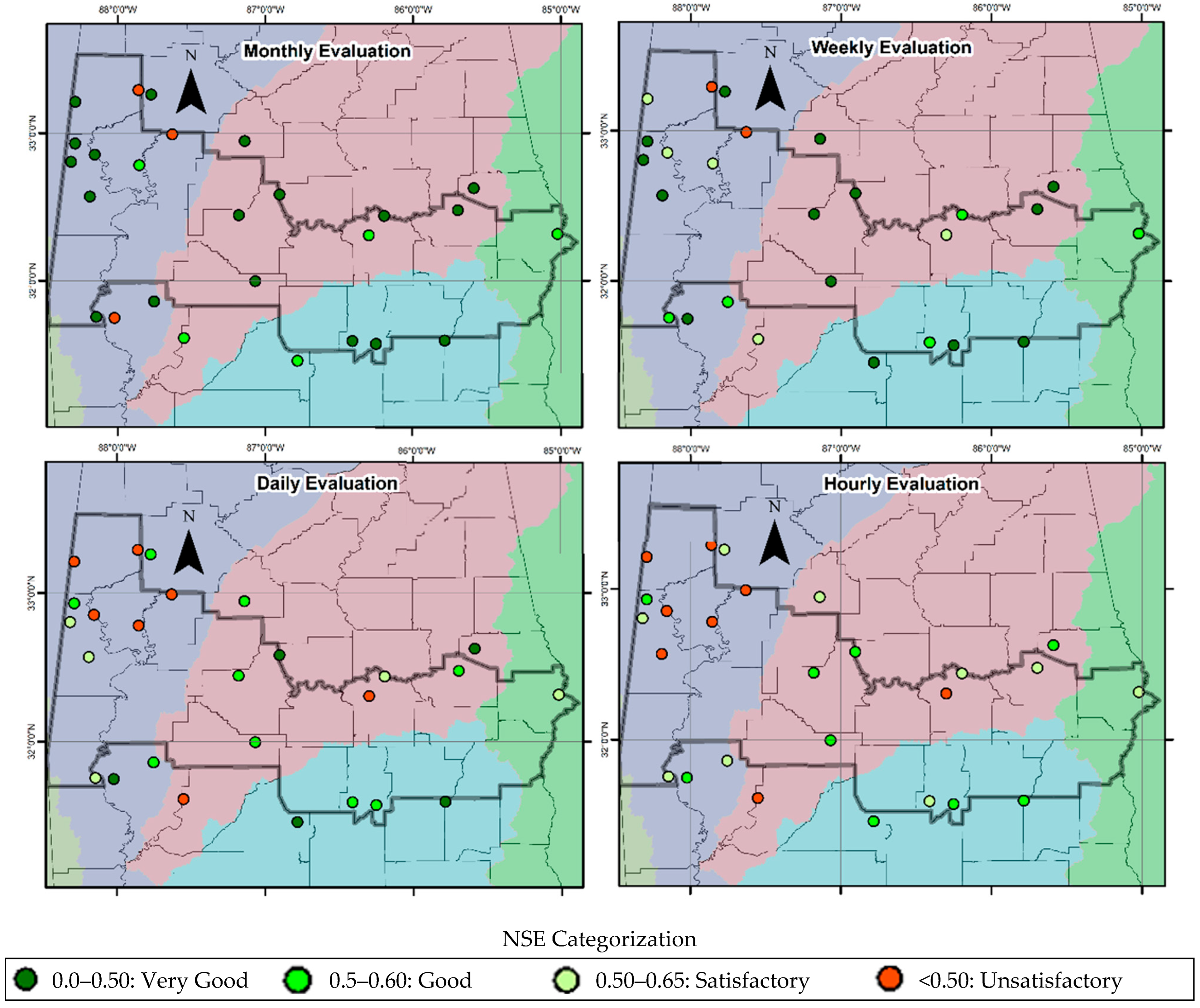
As shown in

Table 2. Heatmap showing NSE performance categories for evaluated locations in the ABBR.

	Hourly	Daily	Weekly	Monthly
Very Good	0%	12%	54%	69%
Good	31%	42%	19%	19%
Satisfactory	38%	19%	19%	0%
Unsatisfactory	31%	27%	8%	12%

and Figure 3 the model’s accuracy improves with coarser temporal scales. On the monthly scale, the majority of locations (88%) had NSE values above good condition (69% very good and 19% good), indicating high proficiency and goodness of fit, between observed and modeled streamflow values. The weekly evaluation showed that 73% of gages had above good model proficiency, with 53.85% of locations with NSE values within the very good category. On the daily scale, the largest proportion of locations (42%) fall into the Good (0.65 ≤ NSE ≤ 0.75) category, suggesting reasonably accurate modeled values for most stations. The hourly simulation evaluation is the most demanding for the model, with 31% of locations classified as Good and another 38% as Satisfactory (0.50 ≤ NSE < 0.65).

The mean NSE, calculated from the data in

Table 3. NSE statistic summary for gages in the ABBR.

USGS Gage	Reach ID (NWM)	NSE
		Hourly	Daily	Weekly	Monthly
02342500	3435970	0.52	0.56	0.66	0.73
02363000	2210130	0.74	0.77	0.82	0.84
02371500	2377281	0.66	0.70	0.80	0.85
02372250	2323396	0.64	0.66	0.75	0.81
02373000	2402121	0.74	0.75	0.83	0.75
02418230	21712124	0.72	0.80	0.85	0.84
02419000	21717690	0.63	0.68	0.78	0.84
02419890	21719268	0.60	0.60	0.66	0.77
02421000	21686584	0.39	0.46	0.61	0.72
02422500	21676818	0.65	0.75	0.80	0.85
02424000	21661814	0.62	0.66	0.82	0.85
02425000	21662336	0.70	0.73	0.86	0.86
02427250	21457950	0.68	0.71	0.77	0.80
02428400	18239649	0.49	0.50	0.56	0.70
02444160	18631042	0.44	0.46	0.64	0.87
02446500	166759201	0.62	0.66	0.81	0.87
02447025	18634030	0.32	0.34	0.52	0.77
02448500	18604196	0.70	0.71	0.83	0.89
02448900	18604744	0.59	0.65	0.77	0.79
02465000	18229923	0.35	0.37	0.50	0.25
02465493	18208346	0.37	0.44	0.46	0.42
02466030	18215736	0.38	0.39	0.51	0.75
02467500	18540822	0.49	0.59	0.77	0.85
02469761	18531726	0.60	0.60	0.69	0.84
02469800	18548516	0.73	0.77	0.82	0.43
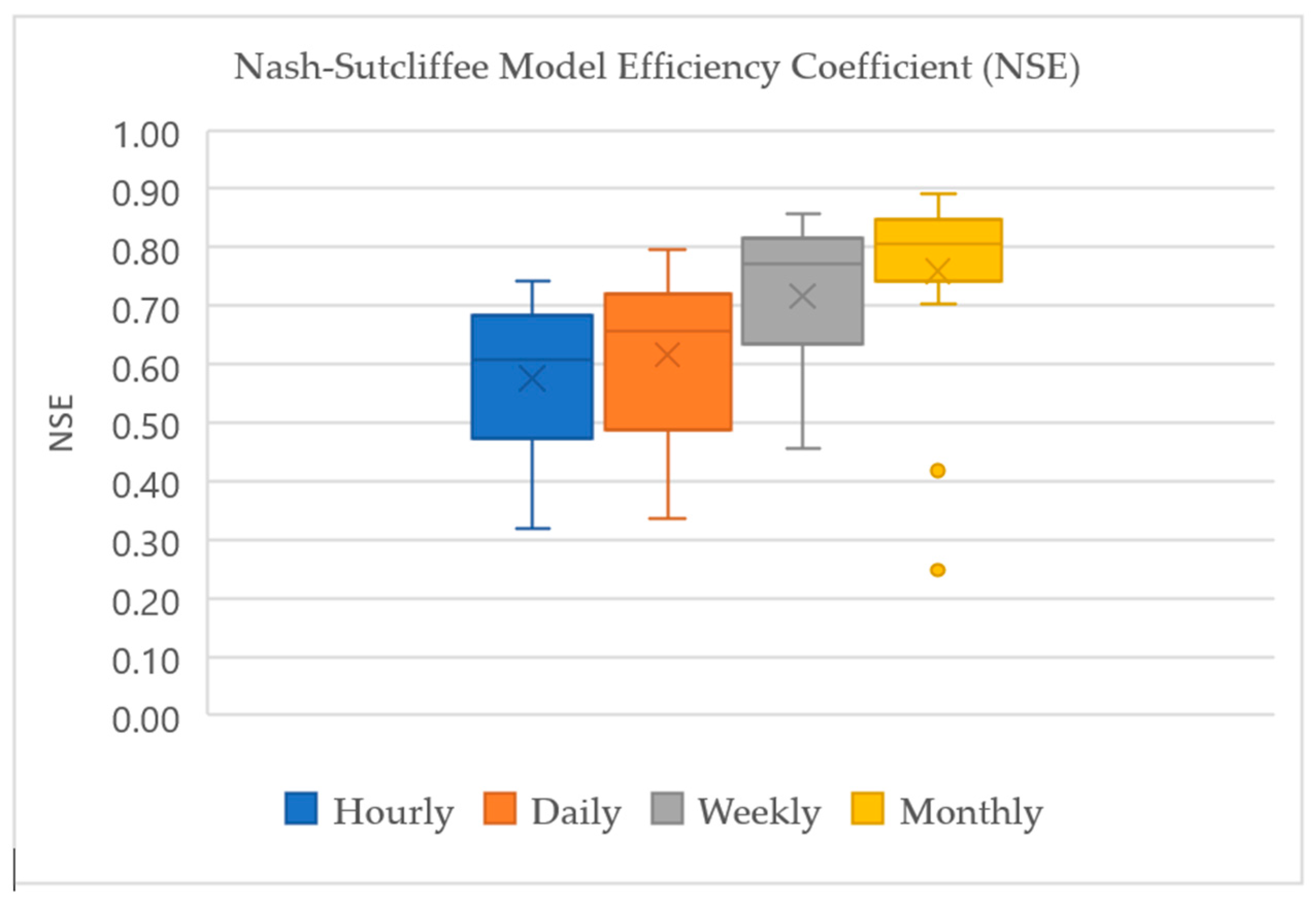
02470072	21640642	0.60	0.71	0.75	0.80

, demonstrates a consistent improvement, ranging from 0.58 on an hourly scale to 0.76 on a monthly scale. This pattern underscores the model’s strength at coarser temporal scales. The variability, as measured by the standard deviation, exhibits a decrease from hourly to weekly scales, indicating enhanced consistency in performance for coarser temporal resolutions. The box plot of NSE (Figure 4) values across timescale provides additional insights into the variability and performance trends. The median NSE values increases from hourly to monthly evaluations, with the median reaching Satisfactory (NSE ≥ 0.50) on the hourly scale but improving to Very Good (NSE > 0.75) on the monthly scale. The interquartile range exhibits a narrowing tendency with increasing temporal aggregation, suggesting enhanced consistency in performance across weekly and monthly scales.

3.1.2. Root Mean Square Error Observation Standard Deviation Ratio

Analyzing the RSR provides a comprehensive evaluation of the hydrological model’s performance at different time scales within the ABBR. Similarly, NWM’s performance improves significantly as the temporal scale becomes coarser (see

Table 4. Heatmap showing RSR performance categories for evaluated locations in the ABBR.

	Hourly	Daily	Weekly	Monthly
Very Good	0%	23%	62%	69%
Good	38%	27%	12%	15%
Satisfactory	31%	23%	12%	0%
Unsatisfactory	31%	27%	15%	12%

), with RSR values decreasing from the hourly scale to the monthly scale (

Table 5. RSR statistic summary for gages in the ABBR.

USGS Gage	Reach ID (NWM)	RSR
		Hourly	Daily	Weekly	Monthly
02342500	3435970	0.69	0.67	0.58	0.52
02363000	2210130	0.51	0.48	0.42	0.40
02371500	2377281	0.58	0.55	0.45	0.39
02372250	2323396	0.60	0.58	0.50	0.44
02373000	2402121	0.51	0.50	0.41	0.50
02418230	21712124	0.53	0.45	0.39	0.40
02419000	21717690	0.61	0.56	0.47	0.40
02419890	21719268	0.64	0.63	0.58	0.48
02421000	21686584	0.78	0.73	0.62	0.53
02422500	21676818	0.59	0.50	0.44	0.39
02424000	21661814	0.62	0.59	0.43	0.39
02425000	21662336	0.55	0.52	0.38	0.37
02427250	21457950	0.57	0.54	0.48	0.44
02428400	18239649	0.72	0.71	0.66	0.55
02444160	18631042	0.75	0.73	0.60	0.36
02446500	166759201	0.62	0.58	0.43	0.37
02447025	18634030	0.82	0.82	0.69	0.48
02448500	18604196	0.55	0.53	0.41	0.33
02448900	18604744	0.64	0.59	0.48	0.45
02465000	18229923	0.81	0.80	0.71	0.87
02465493	18208346	0.79	0.75	0.74	0.76
02466030	18215736	0.79	0.78	0.70	0.50
02467500	18540822	0.72	0.64	0.47	0.39
02469761	18531726	0.63	0.63	0.56	0.39
02469800	18548516	0.52	0.48	0.43	0.75
02470072	21640642	0.64	0.54	0.50	0.45

). Classification thresholds adapted from [49], define satisfactory performance as RSR ≤ 0.70, with ratings ranging from very good (RSR ≤ 0.50) to unsatisfactory (RSR > 0.70). On the hourly scale, only 38.46% of locations achieve a good rating, and none qualified as very good.

As the temporal resolution shifts to daily evaluations, the model improves, with 23% of locations receiving very good ratings and 50% receiving ratings above good. On a weekly scale, performance improves significantly, with 61.54% of locations achieving a very good rating. This improvement reflects the model’s ability to capture medium- to long-term hydrological processes more efficiently than short-term simulations. The monthly evaluation shows the strongest performance, with 85% of locations rated above the good category (69% very good and 15% good). This indicates that the model excels at simulating aggregated hydrological behavior over coarser temporal resolutions, as it smooths the temporal variability.

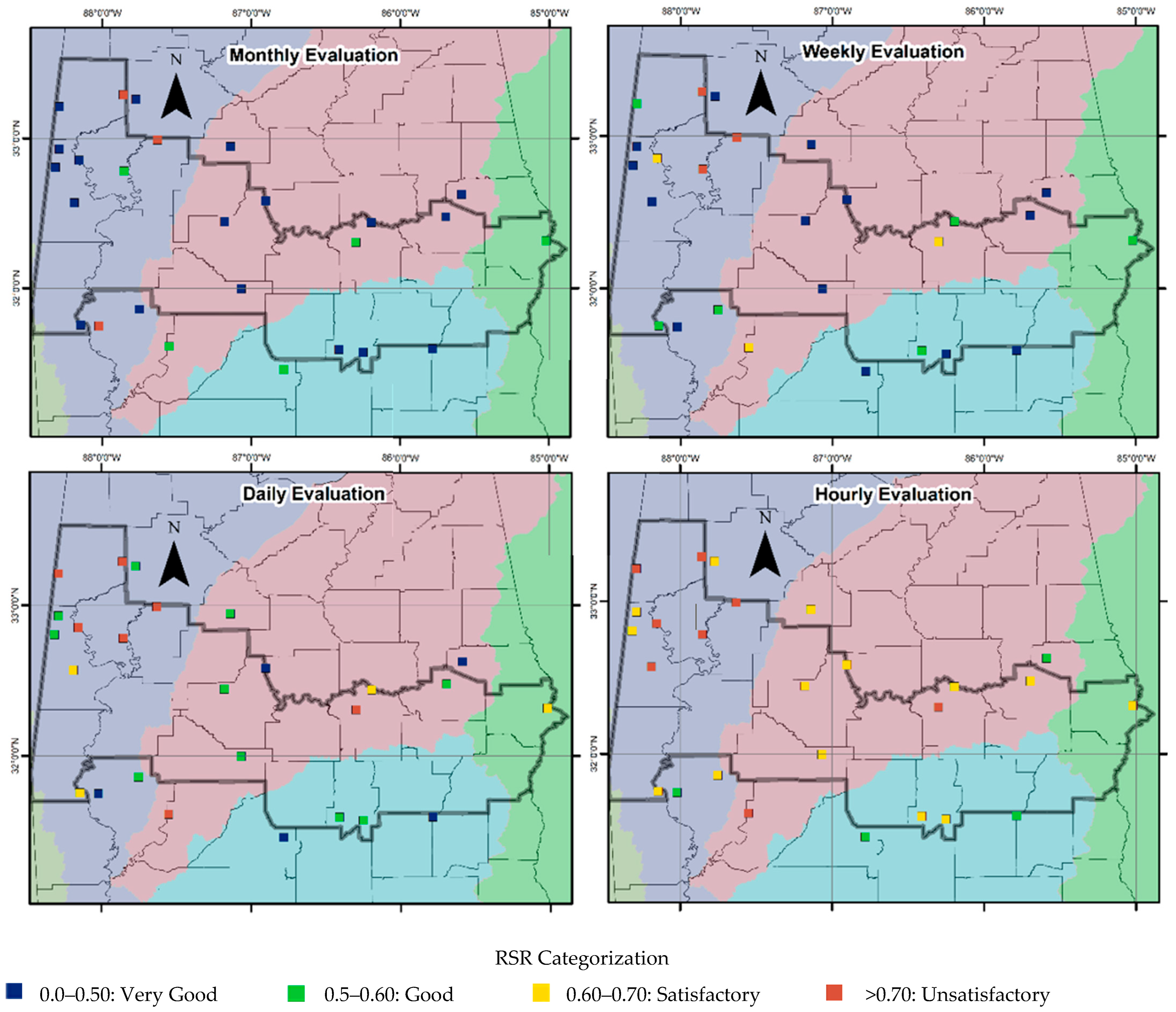
The spatial maps of RSR further highlight regional variations in model performance (Figure 5). Stations in the central and eastern regions consistently attain higher ratings, transitioning from satisfactory or good at finer scales to very good at coarser scales. The box plot for RSR (Figure 6) supports these findings by illustrating the variability and central tendency of RSR values across temporal scales. The median RSR improves steadily, transitioning from satisfactory on the hourly scale to very good on the monthly scale. The interquartile range narrows at coarser temporal resolutions, indicating more consistent performance at the weekly and monthly scales.

3.1.3. Percent BIAS (PBIAS)

The PBIAS values in

Table 6. PBIAS statistic summary for gages within the ABBR.

USGS Gage	Reach ID (NWM)	PBIAS
		Hourly	Daily	Weekly	Monthly
02342500	3435970	−22.5	−22.5	−22.6	−22.7
02363000	2210130	0.0	0.0	0.1	0.1
02371500	2377281	−4.8	−4.8	−5.3	−4.0
02372250	2323396	−14.1	−14.0	−14.1	−14.6
02373000	2402121	−8.3	−8.5	−9.0	−10.4
02418230	21712124	20.1	20.4	20.4	20.4
02419000	21717690	−0.1	0.0	0.1	−0.2
02419890	21719268	−11.2	−11.4	−11.5	−10.9
02421000	21686584	−19.0	−19.1	−19.1	−19.5
02422500	21676818	3.7	3.6	3.4	2.8
02424000	21661814	−5.2	−5.9	−2.5	0.6
02425000	21662336	−3.2	−3.2	−3.7	−4.6
02427250	21457950	−0.7	−0.2	0.3	0.2
02428400	18239649	−6.3	−6.3	−6.2	−6.2
02444160	18631042	−10.5	−10.3	−9.9	−10.0
02446500	166759201	−11.8	−11.8	−11.7	−11.7
02447025	18634030	−11.7	−9.9	−9.8	−8.7
02448500	18604196	−12.3	−12.3	−12.6	−13.6
02448900	18604744	−24.3	−24.0	−23.9	−24.8
02465000	18229923	−6.4	−7.4	−7.3	−20.5
02465493	18208346	−17.7	−17.9	−17.8	−17.6
02466030	18215736	−9.8	−9.8	−9.5	−9.5
02467500	18540822	−16.1	−16.3	−17.0	−16.6
02469761	18531726	−13.4	−13.6	−13.5	−13.6
02469800	18548516	6.5	6.6	6.7	−0.5
02470072	21640642	−2.9	−2.9	−4.3	−5.5

were categorized using the classification thresholds defined in Table 1 for the different temporal resolutions. Percentage bias values were generally similar for specific gages at all time steps. Approximately 70% of the evaluated locations fell within “Very Good” or “Good” categories across all time steps. Notably, no location was classified as “Unsatisfactory” at any temporal scale. Additionally, no clear trend of performance improvement or deterioration was observed with increasing or decreasing temporal aggregation. PBIAS classification levels remained relatively stable from hourly to monthly intervals, with only minor variations in actual values. These results suggest that the NWM maintains a consistent level of bias across time scales, with only minor variations and no significant loss or gain in predictive accuracy.

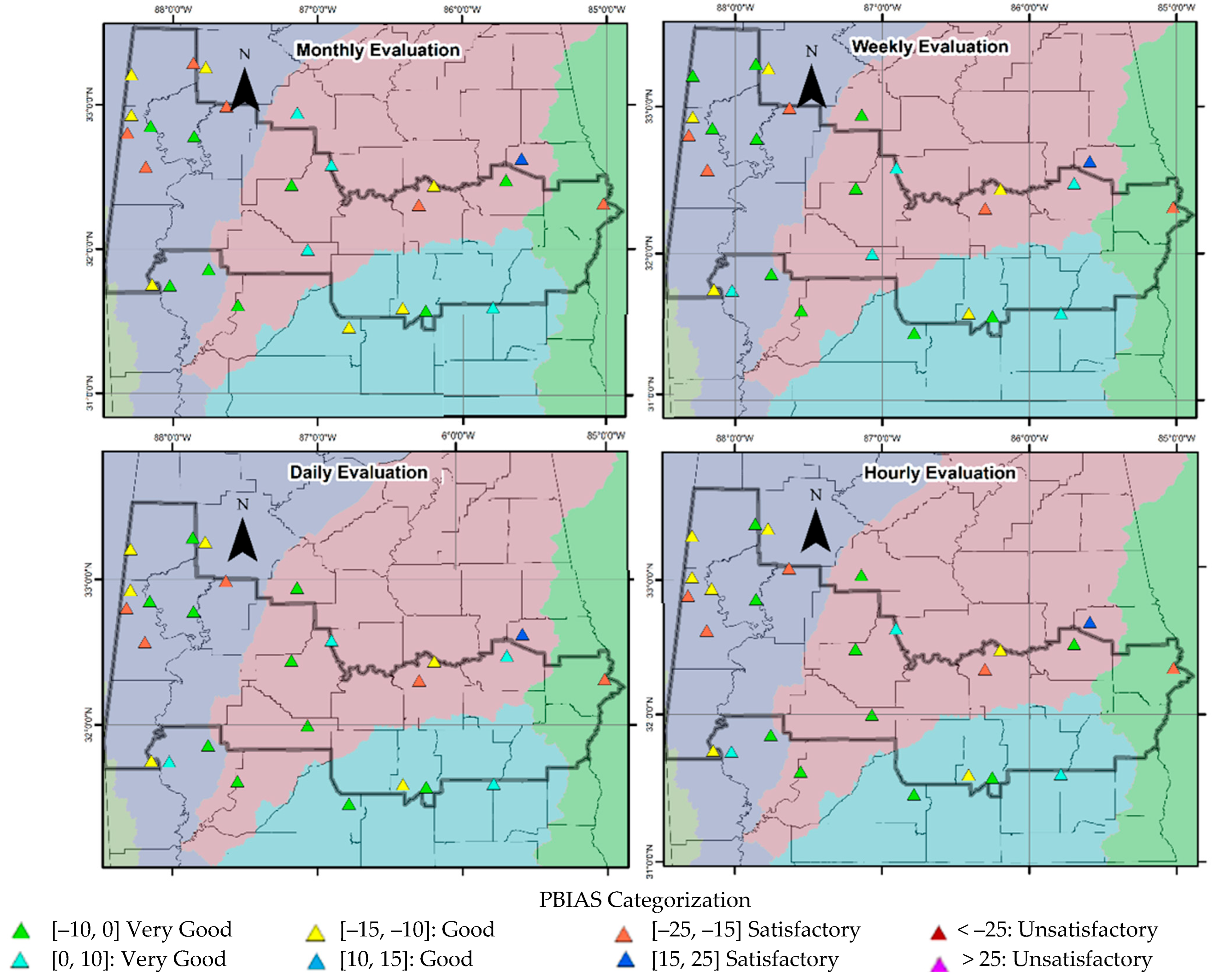
The spatial distribution maps of PBIAS (Figure 7) reveal similar trends in regional variability in model performance across time scales. Central locations consistently receive “Very Good” and “Good” classifications, indicating low bias and high predictive accuracy. The eastern region also shows good performance overall, though with slightly more variability. Notably, no locations were classified as “Unsatisfactory,” indicating that PBIAS remained within acceptable limits across all evaluated stations and time scales.

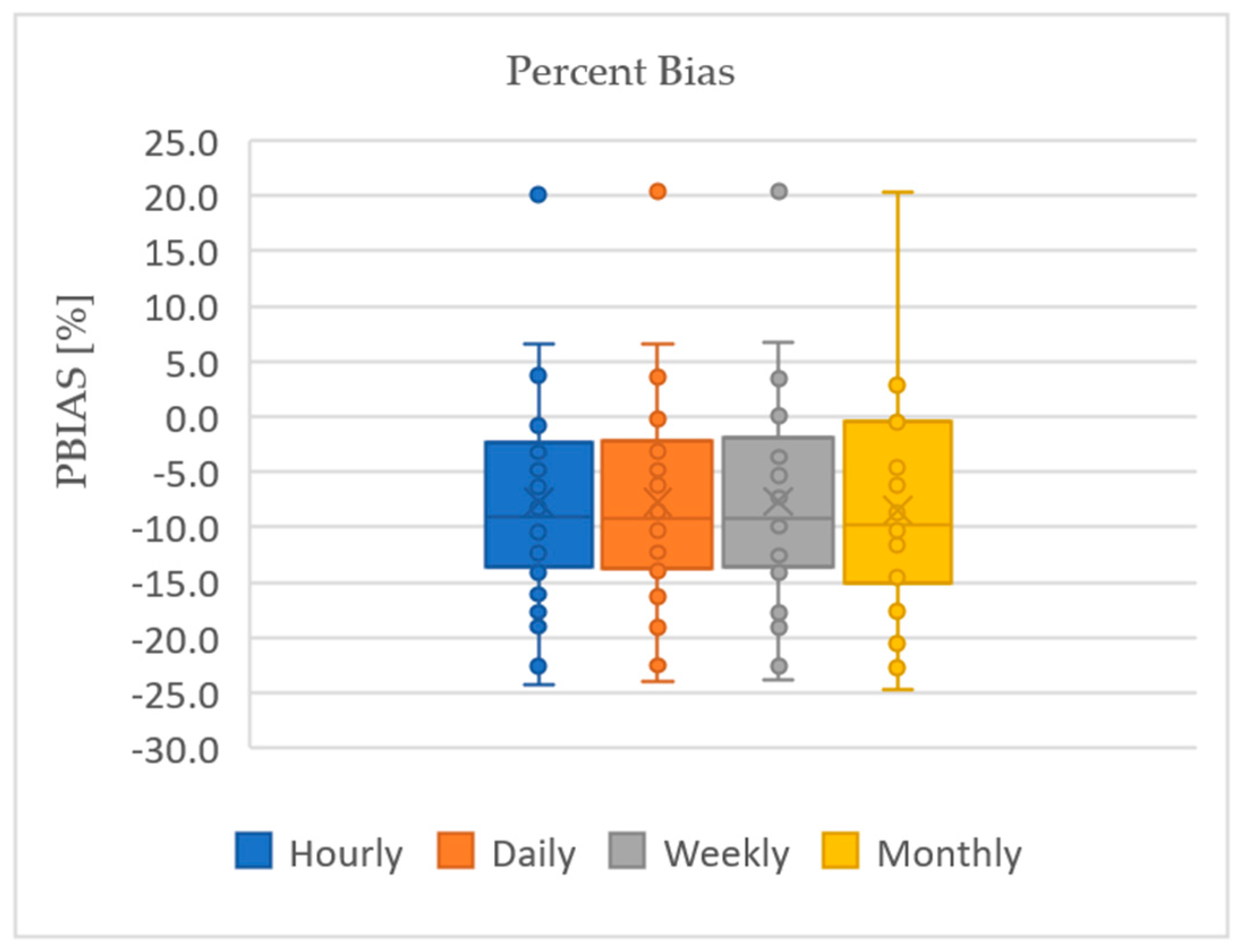
The box plot distribution provides additional context for understanding PBIAS variability across temporal scales (Figure 8). In general, the NWM in the ABBR presented a negative bias for all the temporal scales and locations.

The PBIAS evaluation demonstrates that the NWM performs reliably well for aggregated temporal scales, particularly on a monthly basis, where bias is also minimal. This makes the model well-suited for aggregated temporal hydrological applications, such as water resources planning and seasonal evaluations.

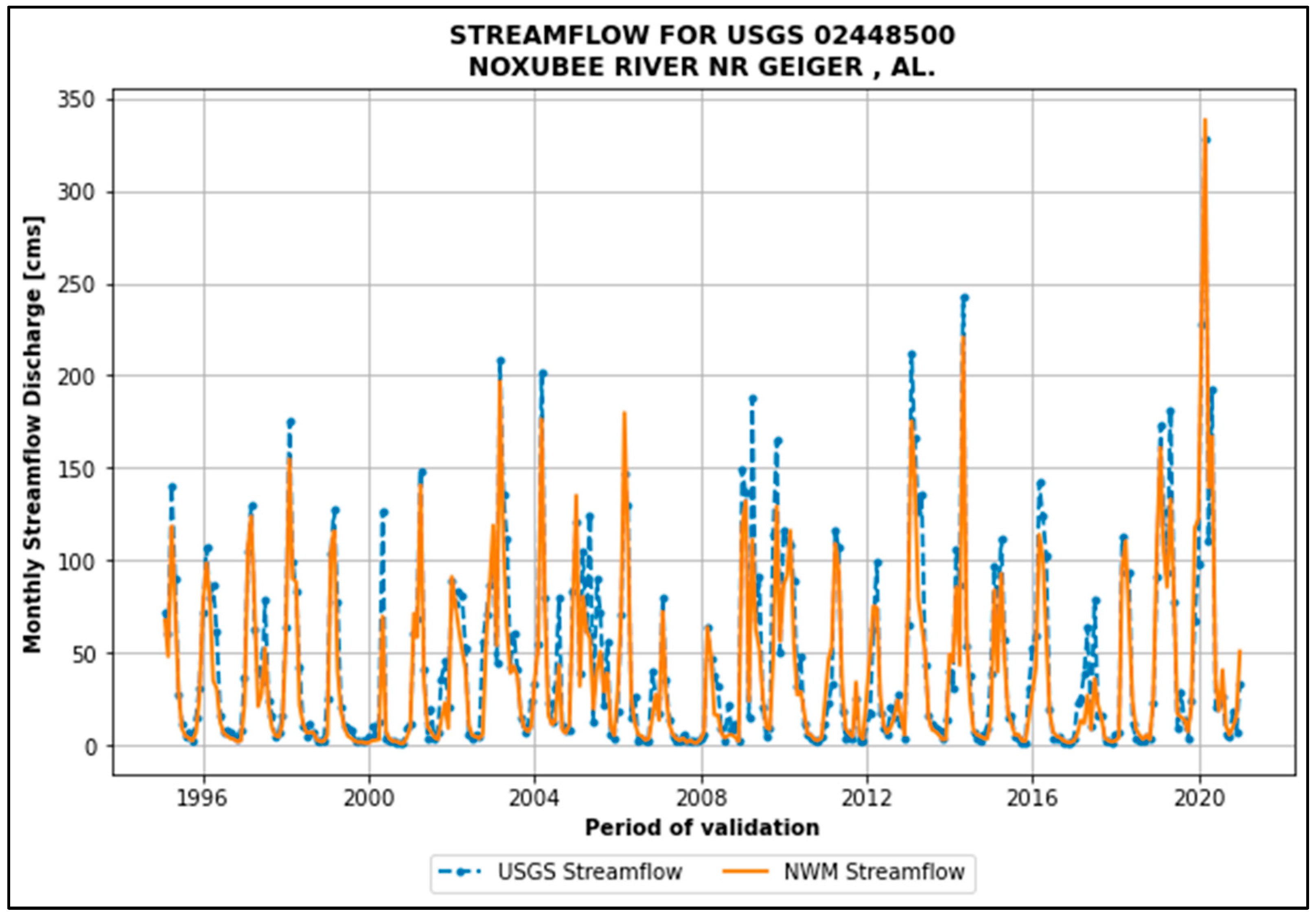
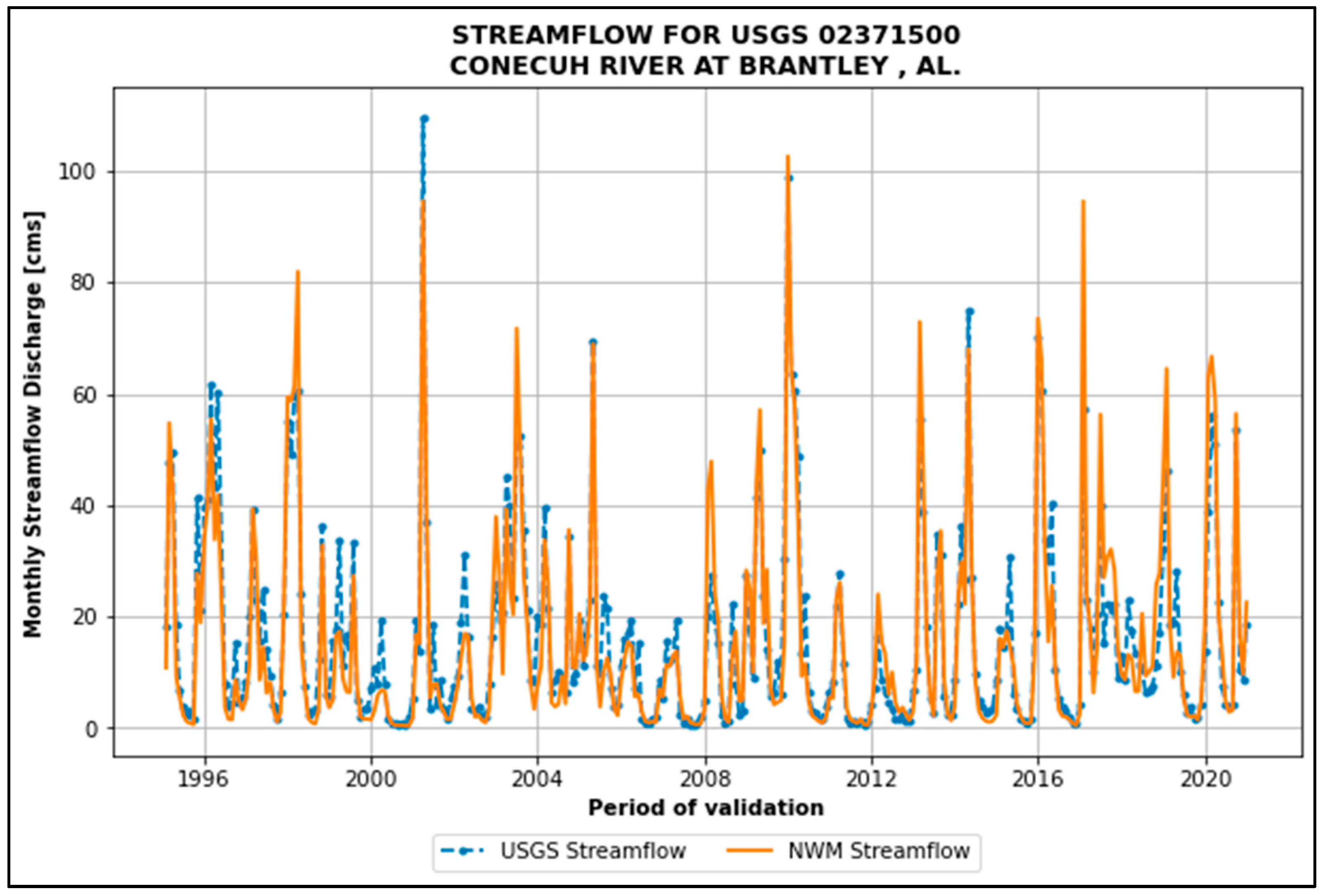
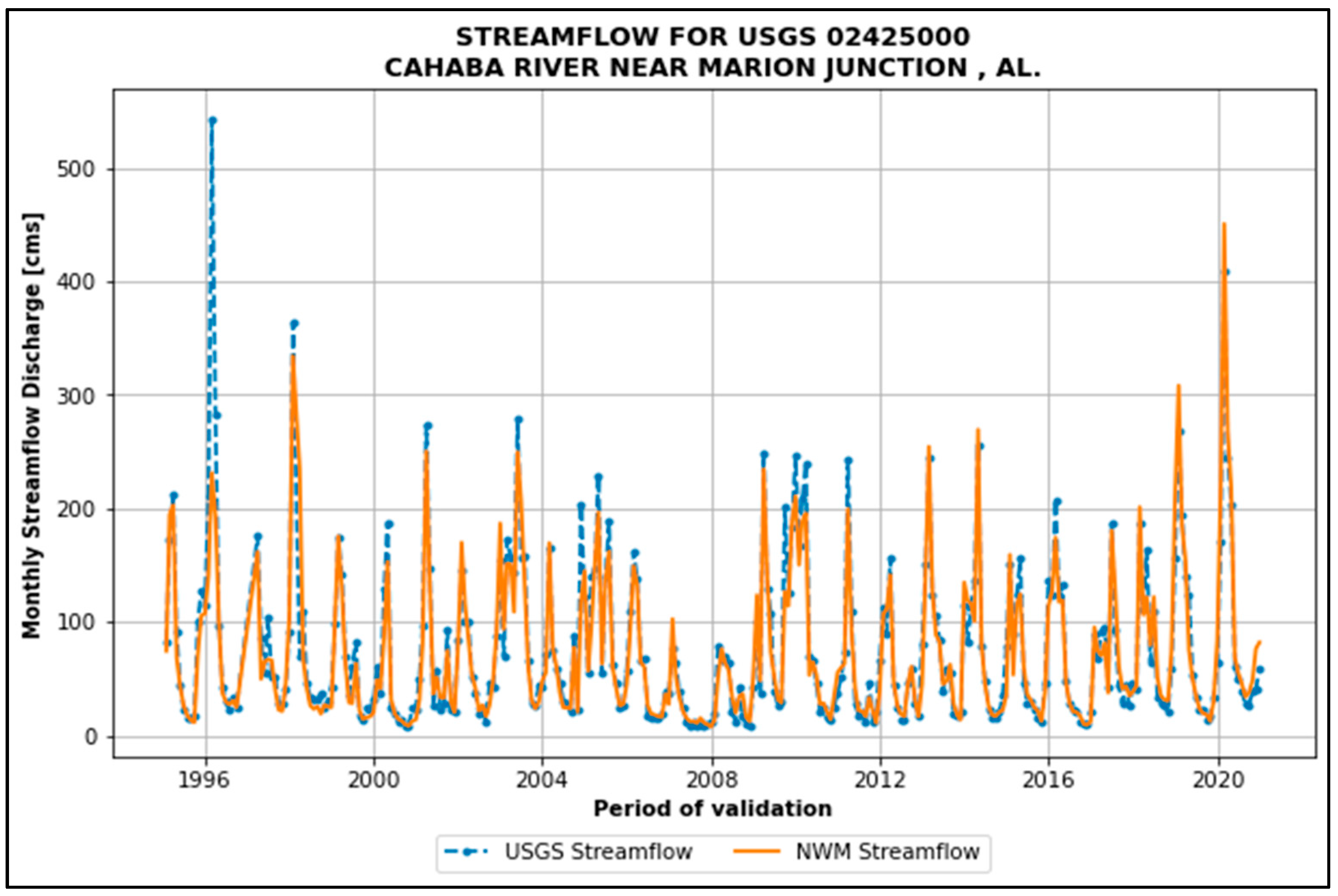
Figure 9, Figure 10 and Figure 11 show monthly streamflow hydrographs for USGS gages and the NWM retrospective data for select reach IDs. The hydrographs provide visual confirmation and goodness of fit of USGS streamflow data against that of NWM. It demonstrates the NMW’s effectiveness in accurately capturing spatial trends, peak events, low flow conditions, and average flow events within the study area.

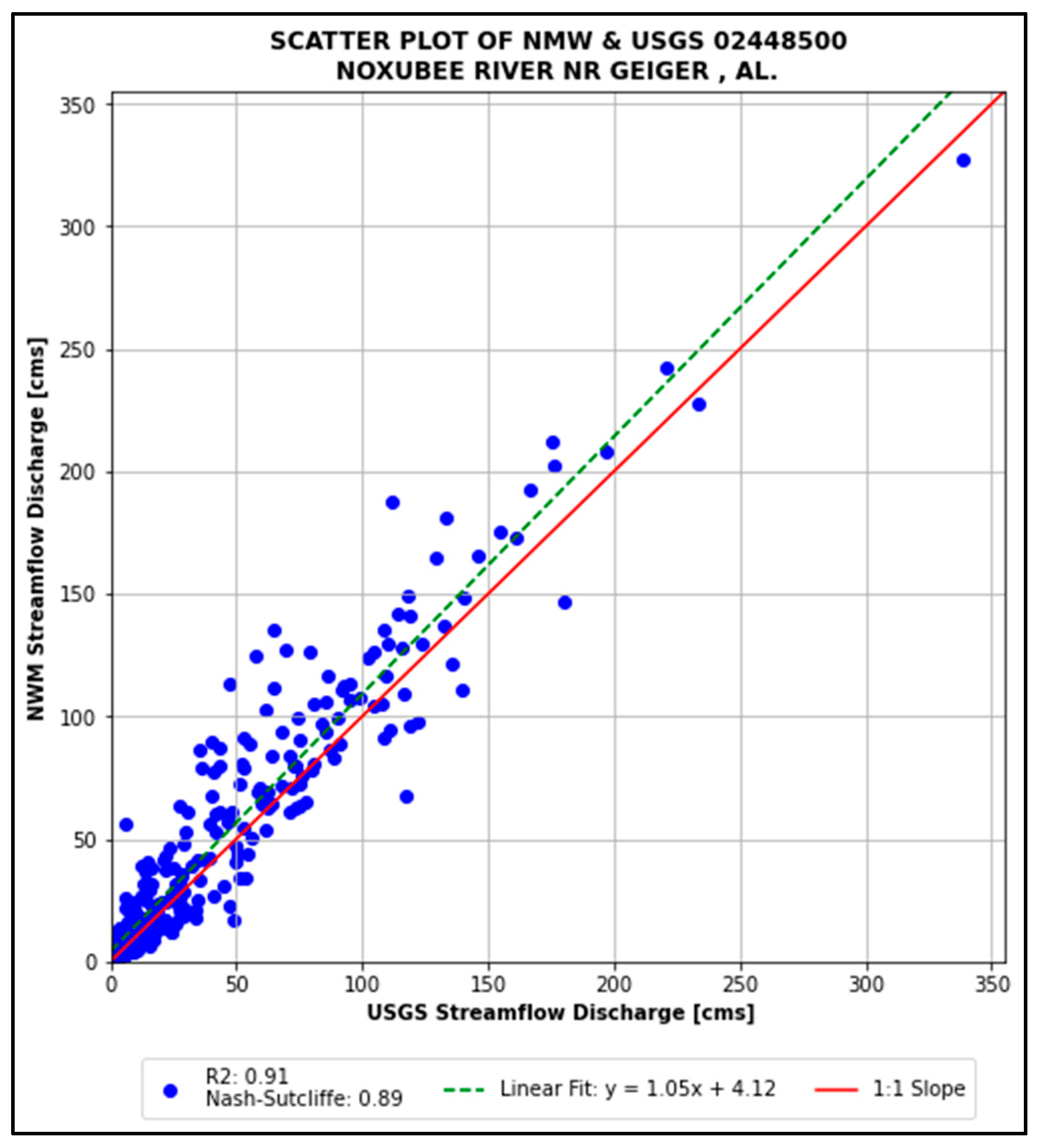
Figure 12, Figure 13 and Figure 14 are the corresponding scatter plots of monthly NWM streamflow data (y-axis) against USGS streamflow data (x-axis) for the reach hydrographs shown in Figure 9, Figure 10 and Figure 11. The scatter plots show high correlation between the NWM and USGS streamflow variables.

4. Discussion

This study provides a detailed evaluation of the NWM within the ABBR, showcasing its strengths and limitations in simulating streamflow dynamics. The results align with prior assessments, such as those by [28], which found that the model performed better in natural flow conditions compared to regulated systems. This study builds on these findings by showing how the NWM performs in a region characterized by diverse hydrological and geological features, and emphasizes the importance of local calibration for effective model application.

The NSE and RSR values showed that the performance of the NWM gets better for coarser temporal resolutions, while the PBIAS tends to be consistent for all timescales, with monthly scale predictions achieving a highest level of agreement with observed USGS streamflow data. Specifically, 69% of the evaluated locations demonstrated “Very Good” performance based on the Nash-Sutcliffe Efficiency (NSE), while Root Mean Square Error Observation Standard Deviation Ratio (RSR) values further confirmed the model’s reliability at this temporal scale. This progression highlights the NWM’s capacity for medium to long-term hydrological forecasting, making it a valuable tool for water resource management and planning.

The evaluation revealed that the NWM’s accuracy against observed data increased with coarser temporal resolutions. Significant variability was observed in hourly and daily evaluations, with performance improving markedly at weekly and monthly scales. This aligns with the understanding that aggregated temporal scales mitigate the influence of short-term variability and input data errors, thereby enhancing model reliability. Spatial analysis also demonstrated consistent performance across the region [28,53] showing good representation of streamflow against measured gages on average.

Similar to previous results [20,29], our study showed that the NWM has a negative bias in the ABBR. Additional factors contributing to the negative bias observed in the ABBR may be linked to structural and anthropogenic limitations in the NWM configuration. Although the model simulates natural hydrological processes with high spatial and temporal resolution, it does not explicitly account for the numerous small- and large-scale human interventions commonly found across the region, such as local dams, reservoirs, agricultural drainage systems, and flow diversions. These modifications can alter streamflow dynamics by attenuating peaks or maintaining higher flows during dry periods—patterns that are not represented in the model’s default setup. Furthermore, the NWM relies on national-scale meteorological forcings, which may underrepresent the magnitude and spatial variability of convective precipitation events that are typical of the southeastern United States. This limitation can result in reduced simulated runoff during short-duration storm events. Although the resulting bias in the ABBR is generally small in magnitude, it remains consistently negative across all evaluated temporal scales. This systematic underestimation suggests the need for improved representation of localized hydrological and anthropogenic processes. Enhancing local and regional calibration, incorporating regulated stream variables data and using higher-resolution meteorological inputs could improve model performance in this complex hydrological setting.

The NWM offers an unprecedented capability to simulate hydrological conditions over 2.7 million stream reaches, supporting nationwide water management and forecasting. Compared to established models like Variable Infiltration Capacity (VIC) and the Sacramento Soil Moisture Accounting (SAC-SMA), the NWM is a more recent and integrated framework, combining distributed physical processes, high-resolution routing, and real-time data assimilation. This architecture enables consistent, large-scale simulations with greater spatial and temporal detail, making it especially suitable for addressing complex, operational hydrologic challenges across diverse regions.

The comprehensive spatial and temporal datasets provided by the NWM are particularly valuable in regions like the ABBR, where limited real-time monitoring infrastructure exists. By bridging data gaps, the model enables informed decisions in flood risk mitigation, drought management, and agricultural planning.

The use of the NWM in water planning, flood risk mitigation, and potentially in agricultural optimization appears promising. While our study focused on evaluating the model’s accuracy, particularly at the coarser temporal resolutions, where it demonstrated high consistency and low variability, these characteristics suggest its potential utility for long-term applications. For example, future research could examine integrating NWM forecasts with socio-economic and ecological datasets to support ecosystem management and ecological change adaptation efforts. The coarser temporal resolutions, with high consistency and low variability, provide a valuable tool for applications that operate on weekly, monthly and seasonal resolutions, including for irrigation and land use management. Additionally, integrating NWM output into hydrological insurance frameworks can provide critical support for risk-based decision-making, and enhance the financial stability of vulnerable communities.

The findings of this study highlight several opportunities for future research and model improvement. Enhancing the representation of regulated flow systems, refining input data quality, and developing region-specific calibration frameworks are critical steps toward improving the NWM’s efficiency and maximizing its utility.

5. Conclusions

This study provides a comprehensive spatiotemporal assessment of the NWM v2.1 streamflow performance across the ABBR. The results confirm that NWM performance improves substantially with temporal aggregation. At the monthly scale, 89% and 85% of stations are rated above “Good” based on NSE and RSR, respectively. These results reinforce the model’s suitability for long-term hydrological applications such as seasonal planning and water resource management. However, a consistent negative bias was observed across all time steps, revealing systematic underestimation of streamflow, particularly in regulated basins and areas with anthropogenic alterations are not explicitly represented in the model structure.

Although the NWM effectively reproduces streamflow variability, its limitations at finer temporal scales and inability to capture regulated flow dynamics underscore the need for regional calibration and enhanced representation of local hydrological processes. The findings underscore the importance of integrating localized land use and infrastructure data, as well as higher-resolution meteorological forcings, to improve predictive accuracy. Future research should focus on adapting the NWM to complex hydrogeological settings through region-specific calibration frameworks and bias correction techniques. Overall, this study demonstrates that the NWM is a valuable tool for operational hydrology in underserved regions. However, its full potential depends on continued model refinement and contextual adaptation.

References

- Fichez, R.; Archundia, D.; Grenz, C.; Douillet, P.; Gutiérrez Mendieta, F.; Origel Moreno, M.; Denis, L.; Contreras Ruiz Esparza, A.; Zavala-Hidalgo, J. Global climate change and local watershed management as potential drivers of salinity variation in a tropical coastal lagoon (Laguna de Terminos, Mexico). Aquat. Sci. 2017, 79, 219–230. [Google Scholar] [CrossRef]
- Pereira, L.S. Water, Agriculture and Food: Challenges and Issues. Water Resour. Manag. 2017, 31, 2985–2999. [Google Scholar] [CrossRef]
- Quansah, J.E.; Naliaka, A.B.; Fall, S.; Ankumah, R.; Afandi, G.E. Assessing Future Impacts of Climate Change on Streamflow within the Alabama River Basin. Climate 2021, 9, 55. [Google Scholar] [CrossRef]
- Ale, B.; Aven, T.; Jongejan, R. Review and discussion of basic concepts and principles in integrated risk management. In Proceedings of the ESREL (European Safety and Reliability Conference), Prague, Czech Republic, 9–17 September 2009; Taylor & Francis: London, UK, 2009. [Google Scholar] [CrossRef]
- Bhakta Shrestha, B.; Sawano, H.; Ohara, M.; Yamazaki, Y.; Tokunaga, Y. Methodology for Agricultural Flood Damage Assessment. In Recent Advances in Flood Risk Management; Abbot, J., Hammond, A., Eds.; IntechOpen: Hamilton, NJ, USA, 2019. [Google Scholar] [CrossRef]
- Uhlir, P.F.; Schröder, P. Open Data for Global Science. Data Sci. J. 2007, 6, OD36–OD53. [Google Scholar] [CrossRef]
- Zipper, S.C.; Stack Whitney, K.; Deines, J.M.; Befus, K.M.; Bhatia, U.; Albers, S.J.; Beecher, J.; Brelsford, C.; Garcia, M.; Gleeson, T.; et al. Balancing Open Science and Data Privacy in the Water Sciences. Water Resour. Res. 2019, 55, 5202–5211. [Google Scholar] [CrossRef]
- USGS; US Department of Interior. National Water Information System: Web Interface; USGS Surface-Water Data for USA: Reston, VA, USA, 2024. Available online: https://waterdata.usgs.gov/nwis/sw (accessed on 25 January 2024).
- Ashraf Vaghefi, S.; Mousavi, S.J.; Abbaspour, K.C.; Srinivasan, R.; Arnold, J.R. Integration of hydrologic and water allocation models in basin-scale water resources management considering crop pattern and climate change: Karkheh River Basin in Iran. Reg. Environ. Change 2015, 15, 475–484. [Google Scholar] [CrossRef]
- Hoyos, N.; Correa-Metrio, A.; Jepsen, S.M.; Wemple, B.; Valencia, S.; Marsik, M.; Doria, R.; Escobar, J.; Restrepo, J.C.; Velez, M.I. Modeling Streamflow Response to Persistent Drought in a Coastal Tropical Mountainous Watershed, Sierra Nevada De Santa Marta, Colombia. Water 2019, 11, 94. [Google Scholar] [CrossRef]
- Karabulut, A.; Egoh, B.N.; Lanzanova, D.; Grizzetti, B.; Bidoglio, G.; Pagliero, L.; Bouraoui, F.; Aloe, A.; Reynaud, A.; Maes, J.; et al. Mapping water provisioning services to support the ecosystem–water–food–energy nexus in the Danube river basin. Ecosyst. Serv. 2016, 17, 278–292. [Google Scholar] [CrossRef]
- Ndulue, E.L.; Mbajiorgu, C.C.; Ugwu, S.N.; Ogwo, V.; Ogbu, K.N. Assessment of land use/cover impacts on runoff and sediment yield using hydrologic models: A review. J. Ecol. Nat. Environ. 2015, 7, 46–55. [Google Scholar] [CrossRef]
- Cosgrove, B.; Gochis, D.; Flowers, T.; Dugger, A.; Ogden, F.; Graziano, T.; Clark, E.; Cabell, R.; Casiday, N.; Cui, Z.; et al. NOAA’s National Water Model: Advancing operational hydrology through continental-scale modeling. JAWRA J. Am. Water Resour. Assoc. 2024, 60, 247–272. [Google Scholar] [CrossRef]
- Bales, J.D.; Flowers, T. Featured Collection Introduction: National Water Model IV. J. Am. Water Resour. Assoc. 2022, 58, 1–4. [Google Scholar] [CrossRef]
- Jachens, E.; Hutcheson, H.; Thomas, M. Groundwater-Surface Water Exchange and Streamflow Prediction using the National Water Model in the Northern High Plains Aquifer region, USA. In National Water Center Innovators Program Summer Institute Report 2018; Columbia Engineering: New York, NY, USA, 2018. [Google Scholar]
- Kopp, S.; Cline, D.; Miniat, C.; Lucero, C.; Rothlisberger, J.; Levinson, D.; Evett, S.; Brusberg, M.; Lowenfish, M.; Strobel, M.; et al. Perspectives on the National Water Model. AWRA Impact 2018, 20, 10–11. [Google Scholar]
- Shastry, A.; Egbert, R.; Aristizabal, F.; Luo, C.; Yu, C.W.; Praskievicz, S. Using Steady-State Backwater Analysis to Predict Inundated Area from National Water Model Streamflow Simulations. JAWRA J. Am. Water Resour. Assoc. 2019, 55, 940–951. [Google Scholar] [CrossRef]
- Zheng, X.; D’Angelo, C.; Maidment, D.R.; Passalacqua, P. Application of a Large-Scale Terrain-Analysis-Based Flood Mapping System to Hurricane Harvey. J. Am. Water Resour. Assoc. 2022, 58, 149–163. [Google Scholar] [CrossRef]
- Viterbo, F.; Mahoney, K.; Read, L.; Salas, F.; Bates, B.; Elliott, J.; Cosgrove, B.; Dugger, A.; Gochis, D.; Cifelli, R. A Multiscale, Hydrometeorological Forecast Evaluation of National Water Model Forecasts of the May 2018 Ellicott City, Maryland, Flood. J. Hydrometeorol. 2020, 21, 475–499. [Google Scholar] [CrossRef]
- Duan, Y.; Kumar, S. Predictability of Seasonal Streamflow and Soil Moisture in National Water Model and a Humid Alabama–Coosa–Tallapoosa River Basin. J. Hydrometeorol. 2020, 21, 1447–1467. [Google Scholar] [CrossRef]
- Dyer, J.; Mercer, A.; Raczyński, K. Identifying Spatial Patterns of Hydrologic Drought over the Southeast US Using Retrospective National Water Model Simulations. Water 2022, 14, 1525. [Google Scholar] [CrossRef]
- Raczynski, K.; Dyer, J. Variability of Annual and Monthly Streamflow Droughts over the Southeastern United States. Water 2022, 14, 3848. [Google Scholar] [CrossRef]
- Garousi-Nejad, I.; Tarboton, D.G. A Comparison of National Water Model Retrospective Analysis Snow Outputs at SNO℡ Sites Across the Western U.S. Hydrol. Process. 2022, 36, e14469. [Google Scholar] [CrossRef]
- Gochis, D.J.; Barlage, M.; Dugger, A.; FitzGerald, K.; Karsten, L.; McAllister, M.; McCreight, J.; Mills, J.; RafieeiNasab, A.; Read, L.; et al. The WRF-Hydro Modeling System Technical Description, 5th ed.; NCAR Technical Note; NCAR: Boulder, CO, USA, 2018; p. 107. Available online: https://ral.ucar.edu/sites/default/files/public/WRF-HydroV5TechnicalDescription.pdf (accessed on 12 February 2024).
- Han, H.; Han, H.; Kim, J.; Chandrasekar, V.; Chandrasekar, V.; Choi, J.; Lim, S. Modeling Streamflow Enhanced by Precipitation from Atmospheric River Using the NOAA National Water Model: A Case Study of the Russian River Basin for February 2004. Atmosphere 2019, 10, 466. [Google Scholar] [CrossRef]
- Hansen, C.; Shafiei Shiva, J.; McDonald, S.; Nabors, A. Assessing Retrospective National Water Model Streamflow with Respect to Droughts and Low Flows in the Colorado River Basin. JAWRA J. Am. Water Resour. Assoc. 2019, 55, 964–975. [Google Scholar] [CrossRef]
- Jachens, E.; Hutcheson, H.; Thomas, M.B.; Steward, D.R. Effects of Groundwater-Surface Water Exchange Mechanism in the National Water Model over the Northern High Plains Aquifer, USA. J. Am. Water Resour. Assoc. 2020, 57, 241–255. [Google Scholar] [CrossRef]
- Lahmers, T.M.; Hazenberg, P.; Gupta, H.; Castro, C.; Gochis, D.; Dugger, A.; Yates, D.; Read, L.; Karsten, L.; Wang, Y.-H. Evaluation of NOAA National Water Model Parameter Calibration in Semiarid Environments Prone to Channel Infiltration. J. Hydrometeorol. 2021, 22, 2939–2969. [Google Scholar] [CrossRef]
- Abdelkader, M.; Temimi, M.; Ouarda, T.B.M.J. Assessing the National Water Model’s Streamflow Estimates Using a Multi-Decade Retrospective Dataset across the Contiguous United States. Water 2023, 15, 2319. [Google Scholar] [CrossRef]
- S.1643-117th Congress (2021–2022): Alabama Black Belt National Heritage Area Act (2021-05-13). Available online: https://www.congress.gov/bill/117th-congress/senate-bill/1643 (accessed on 6 October 2021).
- Gibson, J.S. The Alabama Black Belt: Its Geographic Status. Econ. Geogr. 1941, 17, 1–23. [Google Scholar] [CrossRef]
- Prior, J.W.; Wong, D.W.S. Exploring different dimensions in defining the Alabama Black Belt. GeoJournal 2022, 87, 1525–1542. [Google Scholar] [CrossRef]
- Fall, S.; Abdalla, E.; Quansah, J.; Franklin, M.J.; Whaley-Omidire, T. County-Level Assessment of Vulnerability to COVID-19 in Alabama. ISPRS Int. J. Geo-Inf. 2022, 11, 320. [Google Scholar] [CrossRef]
- Smith, E.A.; Johnson, L.C.; Langdon, D.W., Jr.; Aldrich, T.H.; Cunningham, K.M. Report on the Geology of the Coastal Plain of Alabama; Special Report 6; Brown Printing Company, State Printers: Monterey Park, CA, USA, 1894; p. 759. Available online: https://books.google.com/books?id=BzsxAQAAMAAJ (accessed on 12 February 2024).
- Stephenson, L.W.; Monrow, W.H. Stratigraphy of the Upper Cretaceous series in Mississippi and Alabama; Bulletin V. 22 12; American Association of Petroleum Geologists: Tulsa, OK, USA, 1938; pp. 1639–1657. Available online: https://ngmdb.usgs.gov/Prodesc/proddesc_87938.htm (accessed on 12 January 2024).
- Winemiller, T. Black Belt Region in Alabama. In Encyclopedia of Alabama; Alabama Humanities Alliance: Birmingham, AL, USA, 2009; Available online: https://encyclopediaofalabama.org/article/black-belt-region-in-alabama/ (accessed on 18 February 2024).
- USGS. Hydrologic Unit Codes (HUCs) Explained; USGS: Reston, VA, USA, 2024. Available online: https://nas.er.usgs.gov/about/hucs.aspx (accessed on 12 January 2024).
- NOAA. The National Water Model; OWP Office of Water Prediction: Washington, DC, USA, 2023. Available online: https://water.noaa.gov/about/nwm (accessed on 18 January 2024).
- Gochis, D.J.; Cosgrove, B.; Dugger, A.L.; Karsten, L.; Sampson, K.M.; McCreight, J.L.; Flowers, T.; Clark, E.P.; Vukicevic, T.; Salas, F.; et al. Multi-Variate Evaluation of the NOAA National Water Model; AGU Fall Meeting Abstracts; 2018, H33G-01. Available online: https://ui.adsabs.harvard.edu/abs/2018AGUFM.H33G..01G/abstract (accessed on 24 July 2024).
- NOAA. National Water Model. Available online: https://toolkit.climate.gov/tool/national-water-model (accessed on 16 June 2021).
- Ames, D. Introduction to the National Water Model; Hydrolearn, 2020. Available online: https://apps.edx.hydrolearn.org/learning/course/course-v1:BYU+NWM101+2021/home (accessed on 12 June 2024).
- NOAA. NOAA National Water Model CONUS Retrospective Dataset. 2024. Available online: https://registry.opendata.aws/nwm-archive/ (accessed on 13 June 2024).
- Castronova, A. Visualizing NWM Retrospective Streamflow in Python; Hydroshare. Available online: https://www.hydroshare.org/resource/830b603665cc4ac0893d5449badd422d/ (accessed on 13 June 2024).
- Keown, P. NOAA National Water Model Retrospective Model Data. Available online: https://github.com/NOAA-Big-Data-Program/bdp-data-docs/tree/main/nwm (accessed on 15 November 2021).
- England, J.F.; Cohn, T.A.; Faber, B.A.; Stedinger, J.R.; Thomas, W.O.; Veileux, A.G.; Kiang, J.E.; Mason, R.R. Guidelines for Determining Flood Flow Frequency—Bulletin 17C; 4-B5; Chapter 5 of Section B; Statistical Analysis. Book 4; Hydrologic Analysis and Interpretation; U.S. Geological Survey: Reston, VA, USA, 2019; p. 168.
- Hamilton, A.S.; Moore, R.D. Quantifying Uncertainty in Streamflow Records. Can. Water Resour. J./Rev. Can. Des Ressour. Hydr. 2012, 37, 3–21. [Google Scholar] [CrossRef]
- Helsel, D.R.; Hirsch, R.M.; Ryberg, K.R.; Archfield, S.A.; Gilroy, E.J. Statistical methods in water resources. In Techniques and Methods; 4-A3; Chapter 3 of Section A; Statistical Analysis. Book 4; Hydrologic Analysis and Interpretation; U.S. Geological Survey: Reston, VA, USA, 2020; p. 484. [Google Scholar] [CrossRef]
- Arnold, J.G.; Moriasi, D.N.; Gassman, P.W.; Abbaspour, K.C.; White, M.J.; Srinivasan, R.; Santhi, C.; Harmel, R.D.; Griensven, A.V.; VanLiew, M.W.; et al. Swat: Model Use, Calibration, and Validation. Asabe 2012, 55, 1491–1508. [Google Scholar] [CrossRef]
- Moriasi, D.N.; Arnold, J.G.; Liew, M.W.V.; Bingner, R.L.; Harmel, R.D.; Veith, T.L. Model Evaluation Guidelines for Systematic Quantification of Accuracy in Watershed Simulations. Trans. ASABE 2007, 50, 885–900. [Google Scholar] [CrossRef]
- US EPA, Guidance for Quality Assurance Project Plans for Modeling EPA QA/G-5M [Other Policies and Guidance]. 2015. Available online: https://www.epa.gov/sites/default/files/2015-06/documents/g5m-final.pdf (accessed on 17 June 2015).
- Nash, J.E.; Sutcliffe, J.V. River flow forecasting through conceptual models part I—A discussion of principles. J. Hydrol. 1970, 10, 282–290. [Google Scholar] [CrossRef]
- Gupta, H.V.; Sorooshian, S.; Yapo, P.O. Status of Automatic Calibration for Hydrologic Models: Comparison with Multilevel Expert Calibration. J. Hydrol. Eng. 1999, 4, 135–143. [Google Scholar] [CrossRef]
- Liang, X.; Lettenmaier, D.P.; Wood, E.F.; Burges, S.J. A Simple hydrologically Based Model of Land Surface Water and Energy Fluxes for GSMs. J. Geophys. Res. 1994, 99, 14415–14428. [Google Scholar] [CrossRef]
Figure 1.
(a) State of Alabama showing the ABBR and (b) Hydrologic Basins.
Figure 2.
ABBR showing USGS gage locations in the ABBR.
Figure 3.
Spatial performance trends for NSE statistics.
Figure 4.
Nash-Sutcliffe Model Efficiency Coefficient Box Plot.
Figure 5.
Spatial performance trends for RSR statistics.