Modeling Total Alkalinity in Aquatic Ecosystems by Decision Trees: Anticipation of pH Stability and Identification of Main Contributors

Abstract

Total alkalinity (TAC) plays a pivotal role in buffering acid–base fluctuations and maintaining pH stability in aquatic ecosystems. This study presents a data-driven approach to model TAC using decision tree regression, applied to a comprehensive dataset of 454 water samples collected in diverse aquatic environments of the Médéa region, Algeria. Twenty physicochemical parameters, including concentrations of bicarbonates, hardness, major ions, and trace elements, were analyzed as input features. The decision tree algorithm was optimized using the Dragonfly metaheuristic algorithm coupled with 5-fold cross-validation. The optimized model (DT_DA) demonstrated exceptional predictive performance, with a correlation coefficient R of 0.9999, and low prediction errors (RMSE = 0.3957, MAE = 0.3572, and MAPE = 0.4531). External validation on an independent dataset of 68 samples confirmed the model’s robustness (R = 0.9999; RMSE = 0.4223; MAE = 0.3871, and MAPE = 0.4931). The tree structure revealed that total hardness (threshold: 78.5 °F) and bicarbonate concentration (threshold: 421.68 mg/L) were the most influential variables in TAC determination. The model offers not only accurate predictions but also interpretable decision rules, allowing the identification of critical physicochemical thresholds that govern alkalinity. These findings provide a valuable tool for anticipating pH instability and guiding water quality management and protection strategies in freshwater ecosystems.

1. Introduction

pH stability is a determining factor in maintaining the chemical, biological, and ecological balance of aquatic ecosystems [1,2]. Indeed, many biochemical processes essential to the functioning of aquatic environments are highly dependent on pH, including nutrient bioavailability [3], heavy metal solubility [4], the enzymatic activity of microorganisms [5,6], and the toxicity of various compounds. Any sudden or prolonged variation in pH can have deleterious effects on aquatic flora and fauna, thus affecting the entire food chain [7]. In this context, it becomes crucial to understand, predict, and control the mechanisms underlying pH stability. Among the fundamental parameters regulating this stability is total alkalinity (TAC), a measure of an aqueous system’s buffering capacity to neutralize acids [8]. The TAC is primarily related to the concentration of chemical species such as bicarbonates (HCO₃⁻), carbonates (CO₃²⁻), and hydroxide (OH⁻), which act as regulating chemical reservoirs [9,10]. This buffering capacity is essential for preventing extreme pH fluctuations due to external inputs, such as pollution [11], acid precipitation, or anthropogenic discharges [12]. Monitoring the TAC therefore provides a precise indication of an ecosystem’s chemical resilience to acidic or basic disturbances [13]. TAC modeling is therefore a strategic tool for scientists, water managers, and policymakers, as it offers the ability to predict the buffering capacity of a water body based on measurable physicochemical data [14,15]. However, due to the complexity of the interactions between the multiple environmental parameters that influence alkalinity (temperature, conductivity, concentrations, etc.), traditional approaches based on deterministic equations quickly reach their limits. These methods, often rigid and poorly adaptive, struggle to capture the nonlinear and contextual dynamics of natural systems [16]. It is in this context that artificial intelligence techniques, and more specifically machine learning algorithms, find a privileged field of application [17,18]. These approaches allow the development of flexible predictive models capable of adjusting to data variations and uncovering complex, often non-intuitive, relationships between variables [19]. Among the most interpretable and effective models is the decision tree, a hierarchical classification and regression algorithm that segments the data space based on the most discriminating characteristics [20]. By generating a tree-like structure, this model not only allows for accurate predictions but also provides a detailed understanding of the underlying processes [21]. The main objective of this study is to develop a predictive model based on decision trees to model TAC in surface waters. This modeling aims to provide a reliable and interpretable tool for assessing and maintaining pH stability in various environmental contexts. The proposed approach makes it possible to identify the physicochemical parameters most influential on TAC and to deduce optimal conditions for chemical stability in aquatic environments. Furthermore, the interpretation of decision nodes provides an in-depth understanding of the mechanisms governing pH resilience to exogenous perturbations. The value of this work lies in its ability to reconcile predictive accuracy and interpretability, two criteria that are often at odds with each other in machine learning models. Unlike more complex approaches, such as neural networks or random forests, the decision tree has the advantage of being directly readable by the user. It thus makes it possible to establish simple but effective rules to anticipate variations in TAC, thereby facilitating decision-making in water quality management. Several areas of application can be envisaged based on this model. First, the model allows for a thorough understanding of the relationships between TAC and other physicochemical parameters, highlighting the buffering mechanisms specific to each type of water body. Second, it offers predictive capacity to estimate total alkalinity in situations where certain measurements are unavailable or difficult to obtain. Third, it constitutes a proactive management tool, capable of detecting early signs of pH instability and directing corrective measures before major imbalances occur. Finally, this modeling offers added value for ecosystem preservation by identifying the conditions conducive to maintaining stable alkalinity, and therefore a balanced pH.

The originality of this study lies in several complementary aspects that go beyond the simple use of decision trees or metaheuristic optimization. First, it provides the first targeted application of decision tree modeling to the prediction of total alkalinity (TAC) as a key driver of pH stability in aquatic ecosystems, a critical parameter that has received very limited attention in the modeling literature despite its central role in buffering acid–base fluctuations. Second, the model is not only predictive but also deeply interpretable, offering a transparent, node-by-node analysis of the decision tree that reveals critical physicochemical thresholds such as total hardness and bicarbonate concentration governing water chemical resilience. This capacity to extract explicit, management-ready decision rules represents a significant advance over conventional statistical or “black-box’’ machine-learning approaches, which typically lack explanatory power. Third, the study leverages a unique and extensive one-year database of 454 samples from the hydrogeologically diverse Médéa region, providing a rare opportunity to explore carbonate equilibria under semi-arid conditions where such high-resolution datasets are scarce. This comprehensive sampling captures wide seasonal and spatial variability, enabling the identification of chemical interactions that would remain hidden in smaller or less heterogeneous datasets. Finally, the work introduces an ecosystem-based modeling framework that integrates all influential variables into a single co-dependent system, aligning predictive analytics with the practical needs of water-quality management. By linking interpretable machine learning with operational thresholds, the approach delivers transferable tools for early detection of pH instability and for guiding targeted interventions in the context of climate change, diffuse pollution, urbanization, and freshwater scarcity. Methodologically, the decision tree was rigorously calibrated and optimized using the Dragonfly algorithm with cross-validation and robustness testing, ensuring both exceptional predictive accuracy and reliable generalization to unseen conditions.

2. Materials and Methods

2.1. Sampling Campaign and Study Framework

To develop a robust and reliable predictive model for TAC, an extensive one-year sampling campaign was conducted throughout 2024 across the Médéa region of Algeria. This area is distinguished by its remarkable hydrogeological diversity, encompassing natural springs, rivers, dams, boreholes, and drinking-water treatment plants. A total of 454 water samples were collected, covering both raw and treated waters. Among them, 202 samples were obtained from raw water sources (natural springs, rivers, and dams), while 252 samples were collected from treated waters, primarily originating from drinking-water treatment facilities. This comprehensive sampling strategy ensured wide spatio-temporal coverage of the physicochemical variability of regional water bodies, providing a solid foundation for the development, training, and validation of the predictive models. Although the dataset originates exclusively from the Médéa region, the sampling protocol was specifically designed to capture natural variability on both temporal and spatial scales. Sampling was performed over an entire hydrological year, allowing the model to integrate seasonal and climatic fluctuations, including variations in temperature, precipitation, and hydrological regimes. The Médéa province comprises 64 communes (Figure 1) and spans a wide range of hydrogeological environments, including natural springs, rivers, dams, boreholes, and treated waters. This geographical heterogeneity provides a rich and representative training set, thereby enhancing the internal robustness and generalization capacity of the model.

2.2. Physicochemical Analysis Protocol

All collected samples were analyzed according to the standardized protocols described in the ninth edition of Jean Rodier’s reference work “Water Analysis” [22]. This methodological framework guarantees rigor, reproducibility, and comparability of the results produced. Measurements were carried out in the laboratory under controlled conditions, following the AFNOR standards associated with each parameter [23]. The instruments were systematically calibrated using reference solutions, and all manipulations were performed in duplicate to minimize analytical uncertainties. All data obtained were compiled into a consistent and coherent database.

2.3. Overview of Measured Variables

A total of twenty-one physicochemical parameters were quantified for each sample, covering a representative range of variables affecting water quality. This database includes turbidity, pH, electrical conductivity, total hardness, and concentrations of major cations such as calcium, magnesium, sodium, and potassium, as well as major anions such as bicarbonate, chloride, sulfate, and nitrate. Trace elements such as iron, manganese, and aluminum were also measured, as were broadly indicative parameters such as dry residue, dissolved organic carbon, nitrites, and ammonium. TAC, expressed in °F, was used as the target variable in the modeling.

2.4. Input Variable Selection for TAC Modeling

The TAC modeling phase relied on a rigorous selection of input variables to optimize predictive performance while limiting informational redundancy. To this end, the measured variables were classified into two categories based on their direct or indirect relationship with alkalinity. Direct inputs include pH, as an indicator of acid–base balance influencing the distribution of carbonate species; bicarbonate (HCO₃⁻), which is the main contributor to alkalinity in natural waters; carbonate (CO₃²⁻), if detected under high pH conditions; and calcium (Ca²⁺) and magnesium (Mg²⁺), which interact closely with alkaline species in the system. Indirect inputs include electrical conductivity, which reflects the overall ionic charge, sodium, potassium, chloride, and sulfate ions, which contribute to the overall ionic balance, as well as parameters such as dry residue, dissolved organic carbon, and certain trace elements. Although these do not directly contribute to the definition of the TAC, their presence can affect the physicochemical balance of the solution and therefore indirectly modulate alkalinity.

Building the Training Database

All measured data were structured in

Table 1. The model inputs and output with statistical analysis.

Variables	Symbol	Unit	Min	Mean	Max	STD
Inputs
Electrical conductivity (Cond)	X1	µS/cm	223	1263.98	3570	754.59
Turbidity	X2	NTU	0.10	7.87	1024	58.57
pH	X3	-	2.10	9.62	797	37.07
Total hardness (TH)	X4	°F	8.13	53.42	160	24.27
Calcium (Ca2+)	X5	mg/L	16.03	121.87	360.72	47.40
Magnesium (Mg2+)	X6	mg/L	0	55.20	218.70	36.91
Bicarbonates (HCO3−)	X7	mg/L	6.74	200.11	495.20	117.01
Chlorides (Cl−)	X8	mg/L	10.50	150.76	609.39	125.91
Nitrites (NO2−)	X9	mg/L	0	0.01	0.50	0.07
Ammonium (NH4+)	X10	mg/L	0	0.02	1.05	0.14
Nitrates (NO3−)	X11	mg/L	0	8.13	195.09	15.89
Phosphates (PO43−)	X12	mg/L	0	1.28	288	19.09
Sulfates (SO42−)	X13	mg/L	10.55	342.25	1457	287.37
Sodium (Na+)	X14	mg/L	0	122.05	460	121.67
Potassium (K+)	X15	mg/L	0.005	6.92	805	37.92
Manganese (Mn2+)	X16	mg/L	0	0.007	0.21	0.02
Iron (Fe3+)	X17	mg/L	0	0.013	0.53	0.03
Aluminum (Al+)	X18	mg/L	0	0.005	0.90	0.04
Total dissolved solids (TDS)	X19	mg/L	219.78	1036.23	2895.74	586.87
Organic matter (OM)	X20	mg/L	0	3.26	29.20	3.86
		Output
Total alkalimetric titre (TAC)	Y1	°F	6.50	117.71	663	133.39

, grouping the 20 input variables and the target output, the TAC, to create a usable dataset for modeling. Table 1 presents the selected parameters with their symbols and units of measurement, as well as the results of the descriptive statistical analysis (minimum “min”, mean, maximum “max” and standard deviations “STD” data). This structuring step is crucial, as it allows for the detection of possible outliers, the evaluation of the distribution of variables and the consideration of preliminary treatments such as normalization or logarithmic transformation, in order to guarantee the effectiveness of the prediction algorithms that will be applied subsequently.

2.5. Decision Tree (DT) Method

Decision trees are a supervised learning method widely used in predictive modeling due to their simplicity, robustness, and ability to handle complex data [24]. A decision tree is a tree-like structure in which each internal node corresponds to a condition or test on an explanatory variable, each branch represents an outcome of that test, and each leaf corresponds to a prediction of the target variable [25,26]. This recursive partitioning mechanism divides the input variable space into homogeneous regions based on the target variable [27]. This nonparametric approach makes no prior assumptions about the data distribution or the form of the relationships between variables, making it particularly suited to complex and nonlinear phenomena, often encountered in environmental, hydrological, or chemical fields [28,29]. Unlike traditional statistical analysis methods, such as linear regression, which rely on strict linear relationships and assumptions of normal error, [30,31] decision trees can model nonlinear relationships and complex interactions without prior data transformation [32]. This flexibility makes it possible to capture a wide variety of behaviors, particularly when the effects of variables are not additive, or when critical thresholds condition the behavior of the system under study [33]. For example, in modeling total alkali content (TAC) in water, certain parameters such as pH, bicarbonate, or calcium concentrations can influence TAC in a nonlinear manner and interact with each other, justifying the use of methods capable of identifying these complex structures. One of the major advantages of decision trees lies in their interpretability [34]. Each decision rule corresponds to a simple question that is easy to understand and explain, which is a major asset for researchers and decision-makers who want not only to obtain accurate predictions but also to understand which parameters most influence the outcome [35]. This transparency makes it possible to explore potential causal relationships, identify key variables, and verify the consistency of results with existing theoretical or experimental knowledge. Conversely, several other machine learning algorithms, such as neural networks or support vector machines (SVMs), operate as “black boxes,” whose decisions are difficult to interpret without additional, often complex, analyses [36]. Furthermore, decision trees exhibit high robustness in the face of noisy or incomplete data [37]. They can handle missing values efficiently, either by using built-in imputation methods or by adapting partitioning rules to overcome missing data [38]. Furthermore, trees do not require variable normalization or scaling, which greatly simplifies data preprocessing [39]. This contrasts with other machine learning techniques, which often require careful data preparation to ensure model convergence and performance. The ability of decision trees to handle qualitative and quantitative variables simultaneously is also a significant asset, especially in environmental applications where data may come from different, heterogeneous sources. For example, in a hydrological study, variables such as the presence or absence of certain species, soil type classifications, or continuous measurements such as ion concentration may coexist in the dataset [40]. Decision trees can integrate these different types of variables into a single model without requiring complex coding or specific transformations.

2.5.1. Decision Tree Model Development and Validation

In this study, the DT method was used to predict TAC from the collected physicochemical parameters. The decision tree is a supervised learning algorithm particularly suited to environmental data, as it allows the modeling of nonlinear relationships between variables while remaining interpretable. This method also offers great flexibility in data manipulation and can handle both quantitative and qualitative variables.

Data Preparation

Prior to modeling, the dataset of 454 samples was subjected to a descriptive statistical analysis to ensure data consistency. No abnormal or unrealistic values were identified. All input variables were normalized to the [0–1] range using a min–max scaling method to balance the contribution of parameters with different units and magnitudes. By standardizing the data in this way, it is ensured that each parameter contributes equally to the construction of the tree, which improves the stability and convergence of the algorithm [41]. No logarithmic transformation was applied, as decision trees do not require normality of distributions or linearization of relationships.

Internal Validation

One of the major challenges in predictive modeling is avoiding overfitting, a phenomenon by which a model adapts too closely to the training data to the detriment of its ability to generalize to new data. To mitigate this risk, K-fold cross-validation was implemented, with K set to 5. This technique involves dividing the dataset into five distinct and balanced subsets. The complete dataset of 454 water samples was first randomly shuffled to remove any ordering effects related to sampling location or time. The shuffled data were then split into five subsets (folds) of approximately equal size (about 90 samples per fold). For each iteration, four folds (≈80% of the data) were used as the training set to build the model, while the remaining fold (≈20%) served as the validation set. This procedure was repeated five times, each time rotating the validation fold so that every observation was used once for validation and four times for training. After the five iterations, the performance metrics were computed for each fold and then averaged to provide a stable and unbiased estimate of the model’s predictive accuracy [42].

Hyperparameter Optimization

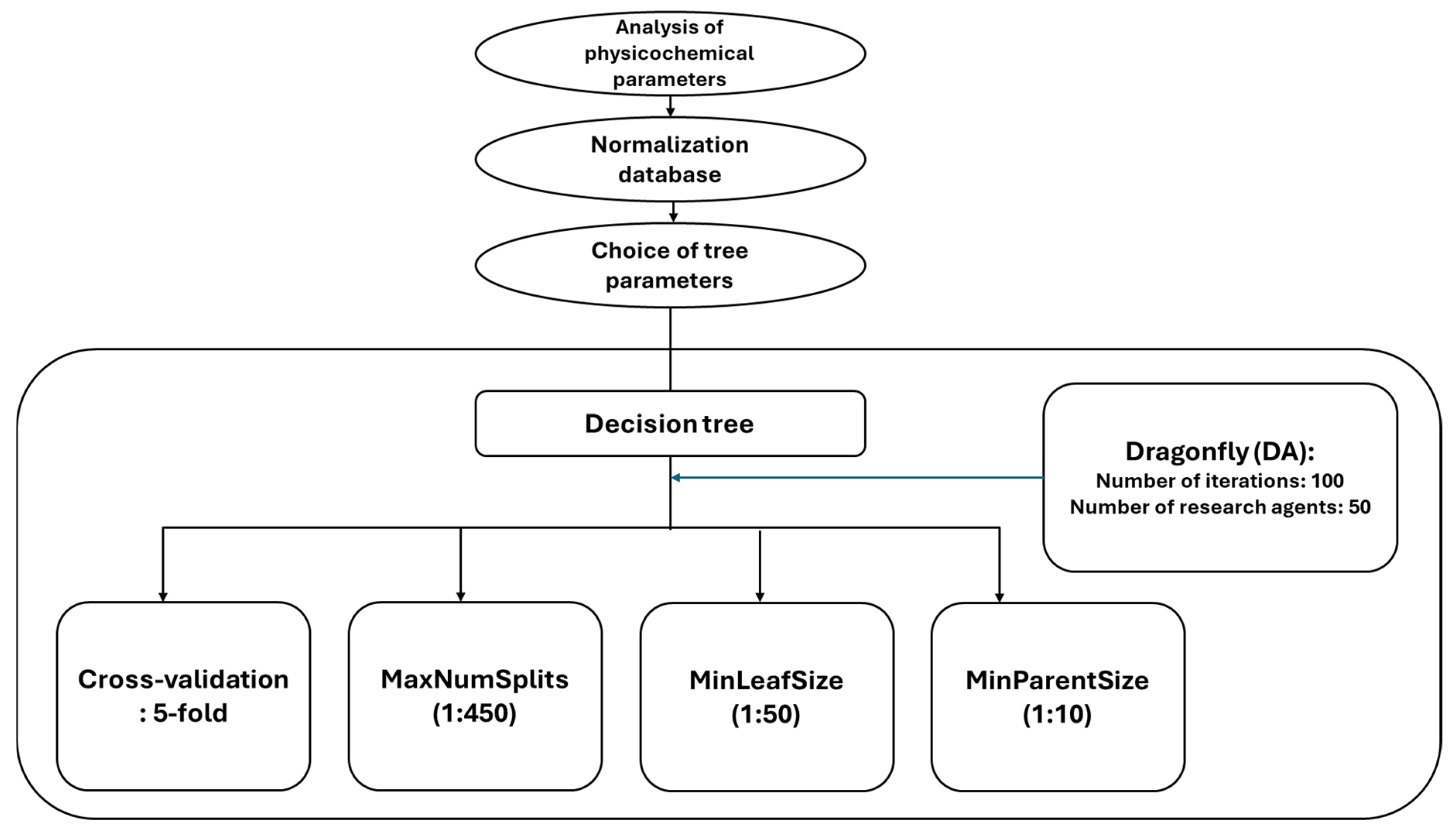
To obtain an optimal model, it is crucial to adjust certain hyperparameters of the decision tree that determine its complexity and predictive capacity. These parameters include the maximum number of splits or cuts (max split), the minimum leaf size, and the minimum number of observations required to generate a branch node. These parameters control the depth and structure of the tree, directly influencing the accuracy and generalization of the model. To optimize these hyperparameters efficiently and systematically, the Dragonfly metaheuristic algorithm was used. Inspired by the collective behavior of dragonflies, this algorithm is distinguished by its ability to efficiently explore the parameter space, avoiding local minima and accelerating convergence towards optimal solutions. Thanks to this automated optimization, it is possible to identify the best combination of hyperparameters that maximize model performance while avoiding overfitting. The hyperparameters subject to optimization and their respective ranges were carefully defined upstream. Figure 2 illustrates these search ranges, specifying the minimum and maximum bounds for each parameter. This delimitation ensures that the optimization search is carried out in a relevant space, thus limiting the risks of excessive exploration or optimization on unrealistic values. This step is fundamental to balance model complexity and performance.

External Validation

The final optimized model was further tested on an independent set of 68 samples not used during training or cross-validation. These samples were collected during the same hydrological year from additional sites in the Médéa region, covering diverse aquatic environments such as natural springs, rivers, dams, boreholes, and treated waters originating from drinking-water treatment plants. Importantly, these locations were different from those used for model training to ensure that the external validation truly tested the model’s transferability to unseen conditions. Predictions obtained from the five best models were averaged to ensure stable estimates. The external validation confirmed the model’s generalization ability, as reflected by a high correlation between predicted and observed TAC values and low error statistics.

Performance Metrics

To rigorously evaluate the predictive performance of the developed models and to identify the most reliable approach, a comprehensive set of statistical indicators was employed. These included the correlation coefficient (R), the coefficient of determination (R²), the adjusted coefficient of determination (R²adj), the root mean square error (RMSE), the mean absolute error (MAE), and the mean absolute percentage error (MAPE). Together, these metrics provide complementary information on both the strength of the association between observed and predicted values and the magnitude of the prediction errors. The mathematical formulations used to compute each criterion are detailed below:

$$\mathrm{R}={\displaystyle \frac{{\displaystyle \sum _{\mathrm{i}=1}^{\mathrm{N}}\left({\mathrm{y}}_{\exp }-{\overline{\mathrm{y}}}_{\exp }\right)\left({\mathrm{y}}_{\mathrm{p}\mathrm{r}\mathrm{e}\mathrm{d}}-{\overline{\mathrm{y}}}_{\mathrm{p}\mathrm{r}\mathrm{e}\mathrm{d}}\right)}}{\sqrt{{\displaystyle \sum _{\mathrm{i}=1}^{\mathrm{N}}{\left({\mathrm{y}}_{\exp }-{\overline{\mathrm{y}}}_{\exp }\right)}^2{\displaystyle \sum _{\mathrm{i}=1}^{\mathrm{N}}{\left({\mathrm{y}}_{\mathrm{p}\mathrm{r}\mathrm{e}\mathrm{d}}-{\overline{\mathrm{y}}}_{\mathrm{p}\mathrm{r}\mathrm{e}\mathrm{d}}\right)}^2}}}}}$$

$$\begin{gathered} {\mathrm{R}}_{\mathrm{a}\mathrm{d}\mathrm{j}}^2=1-{\displaystyle \frac{\left(1-{\mathrm{R}}^2\right)\left(\mathrm{N}-1\right)}{\mathrm{N}-\mathrm{K}-1}} \\ \mathrm{R}\mathrm{M}\mathrm{S}\mathrm{E}=\sqrt{\left({\displaystyle \frac{1}{\mathrm{N}}}\right)\left({\displaystyle \sum _{\mathrm{i}=1}^{\mathrm{N}}{\left[\left({\mathrm{y}}_{\exp }-{\mathrm{y}}_{\mathrm{p}\mathrm{r}\mathrm{e}\mathrm{d}}\right)\right]}^2}\right)} \end{gathered}$$

$$\mathrm{M}\mathrm{A}\mathrm{E}=\left({\displaystyle \frac{1}{\mathrm{N}}}\right){\displaystyle \sum }_{\mathrm{i}=1}^{\mathrm{N}}\left|{\mathrm{y}}_{\exp }-{\mathrm{y}}_{\mathrm{p}\mathrm{r}\mathrm{e}\mathrm{d}}\right|$$

$$\mathrm{M}\mathrm{A}\mathrm{P}\mathrm{E}=\left({\displaystyle \frac{100}{\mathrm{N}}}\right){\displaystyle \sum _{\mathrm{i}=1}^{\mathrm{N}}\left|\frac{{\mathrm{y}}_{\exp }-{\mathrm{y}}_{\mathrm{p}\mathrm{r}\mathrm{e}\mathrm{d}}}{{\mathrm{y}}_{\exp }}\right|}$$

where N is the number of data samples; K is the number of variables (inputs); ${\mathrm{y}}_{\exp }$ and ${\mathrm{y}}_{\mathrm{p}\mathrm{r}\mathrm{e}\mathrm{d}}$ are the experimental and the predicted values, respectively; ${\overline{\mathrm{y}}}_{\exp }$ and ${\overline{\mathrm{y}}}_{\mathrm{p}\mathrm{r}\mathrm{e}\mathrm{d}}$ are, respectively, the average values of the experimental and the predicted values [14,43,44,45].

3. Results

3.1. Decision Tree Modeling

The results of this optimization phase, including the obtained performances and the corresponding parameters, are presented in

Table 2. Performances of the best DT_DA model.

DA Number of Iterations: 100 Number of Research Agents: 50
Min Leaf Size	Surrogate	Min Parent Size	Max Number Splits	Number of Node	R/R2/R2adj			RMSE/MAE/MAPE
					Train	VAL	ALL	Train	VAL	ALL
1	ALL	2	450	427	0.99999 0.99998 0.99997	0.99999 0.99998 0.99997	0.99999 0.99998 0.99997	0.3854 0.3439 0.4392	0.4159 0.3794 0.4731	0.3957 0.3572 0.4531

.

The results obtained from the best decision tree model optimized by the Dragonfly algorithm (DT_DA), presented in Table 2, demonstrate exceptional predictive performance. A 5-fold cross-validation procedure was applied to ensure model robustness and to prevent overfitting. This approach involves training five independent models on different subsets of the data and computing final predictions as the average of the five decision trees, thereby improving the generalization ability of the final model.

The optimized model exhibits near-perfect predictive accuracy across all phases. The R reaches 0.99999 for the training, validation, and combined datasets, while the R² and the R²adj remain equally high at 0.99998 and 0.99997, respectively. Such values indicate that the model captures virtually all of the variability in TAC and accurately reproduces the complex, nonlinear relationships among the physicochemical predictors.

Error metrics confirm this outstanding performance. The RMSE is extremely low, with values of 0.3854 for training, 0.4159 for validation, and 0.3957 overall. Similarly, the MAE remains very small 0.3439 for training, 0.3794 for validation, and 0.3572 overall indicating that, on average, the model’s predictions deviate by less than half a TAC unit from measured values. The MAPE, which expresses errors in relative terms, is also impressively low: 0.4392% in training, 0.4731% in validation, and 0.4531% overall. These extremely low error rates confirm that the model delivers high accuracy with excellent stability, even on previously unseen data.

The close agreement between training and validation metrics demonstrates the absence of overfitting and attests to the model’s ability to generalize effectively. This is further supported by the 5-fold cross-validation procedure, which consistently produced very similar results across all folds [46].

The final DT_DA model was obtained after 100 iterations of the Dragonfly optimization algorithm, using 50 search agents to explore the hyperparameter space. The optimal configuration included a minimum leaf size of 1, a minimum of 2 observations per parent node, and a maximum of 454 splits, with the Surrogate: ALL option enabled so that all available variables could serve as surrogate splitters. This setting enhances the model’s capacity to handle potential missing or noisy data without compromising predictive accuracy.

Altogether, these results highlight that the combination of a decision tree with Dragonfly-based hyperparameter optimization produces a powerful, interpretable, and highly reliable predictive tool for estimating TAC from routine physicochemical water parameters. Figure 3 graphically illustrates the strong agreement between predicted and experimental values across the training, validation, and overall datasets, where the inclusion of R, R²,R²_adj RMSE, MAE, and MAPE values within the panels further reinforces the immediate readability of the model’s exceptional performance.

3.2. External Validation

The results of this comparison, highlighting the consistency between the experimental data and the model outputs, are clearly presented in

Table 3. Model test performance of DT_DA model.

R	R2	R2adj	RMSE	MAE	MAPE
0.99999	0.99998	0.99997	0.4223	0.3871	0.4931

.

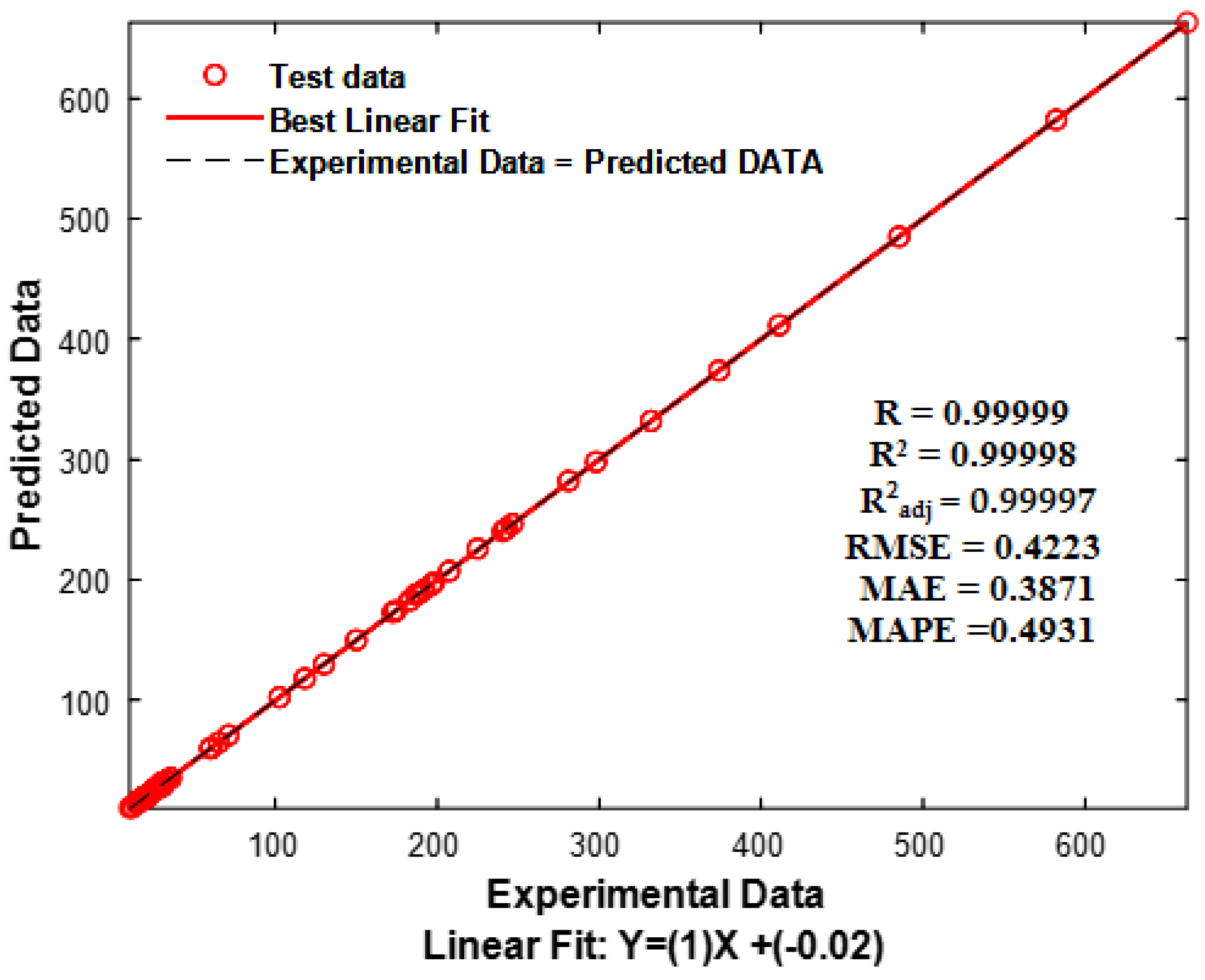
The results presented in Table 3 confirm the remarkable predictive capability of the DT_DA model when applied to a completely independent external dataset that was not used at any stage of model development. The R reaches 0.99999, demonstrating an almost perfect agreement between predicted and measured TAC values and indicating that the model successfully captures the underlying relationships between the physicochemical parameters and total alkalinity. This near-perfect correlation is further supported by a R² of 0.99998 and an adjusted R² of 0.99997, both of which confirm that virtually all of the variance in the experimental data is explained by the model, even after adjusting for model complexity. Error-based metrics reinforce this outstanding performance. The RMSE is exceptionally low at 0.4223, while the MAE is only 0.3871, indicating that the average deviation between predicted and observed TAC values is less than half a unit. Furthermore, the MAPE remains very small at 0.4931%, demonstrating that prediction errors are negligible relative to the magnitude of the measured concentrations. These results clearly show that the DT_DA model is not only highly accurate but also robust and generalizable. The close alignment of these external-test metrics with those obtained during training and cross-validation confirms that the model maintains its predictive power when exposed to new, unseen data, thereby eliminating concerns of overfitting. In summary, Table 3 provides compelling evidence that the DT_DA model, optimized through the Dragonfly algorithm and validated by an independent dataset, offers a solid and reliable predictive framework for estimating TAC. Its combination of near-perfect correlation, extremely low error levels, and proven external validity underscores its suitability as a practical decision-support tool for monitoring and managing water quality in diverse environmental contexts. Figure 4 represents the test performance of DT_DA model graphically.

3.3. Analysis of Model Residuals

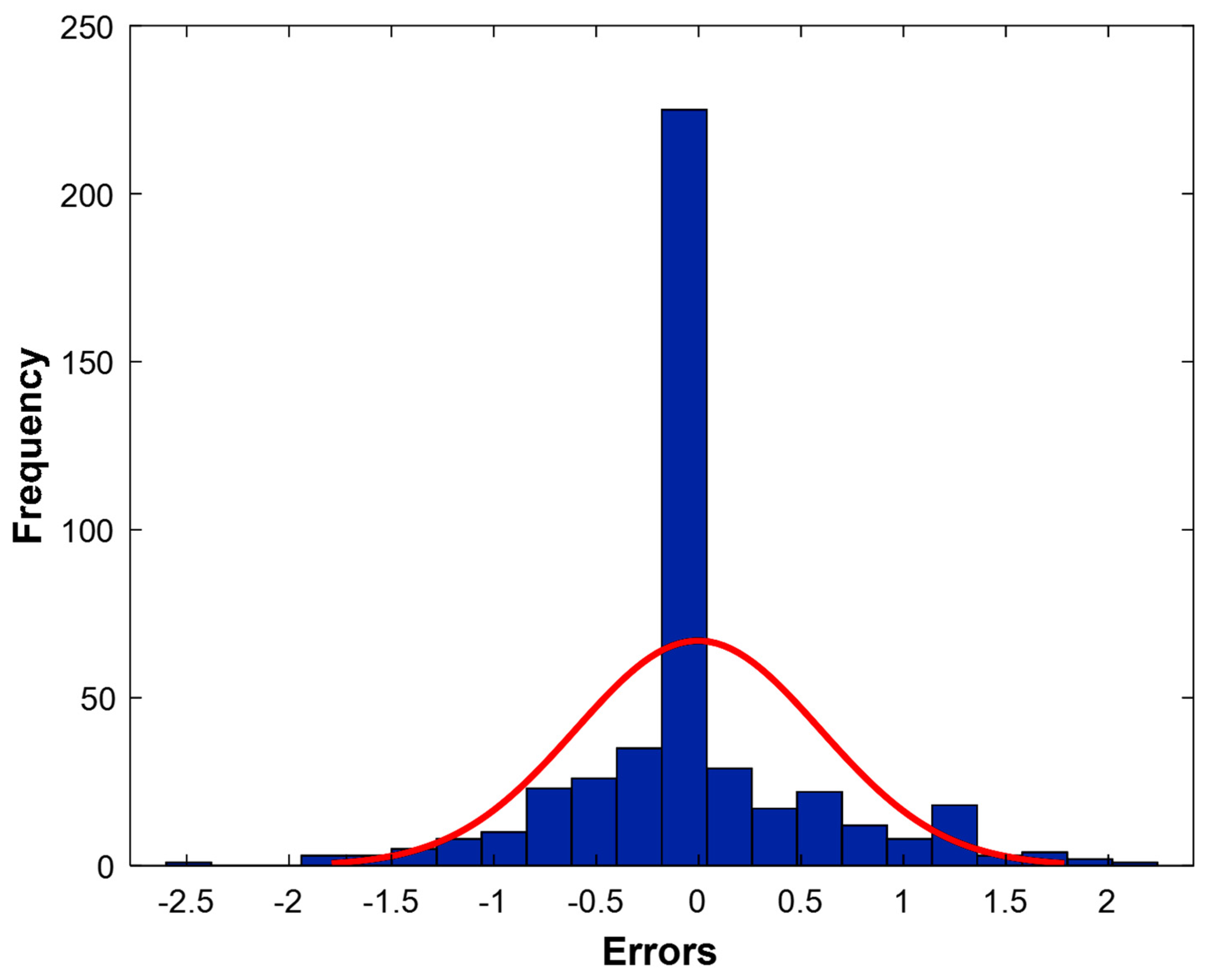
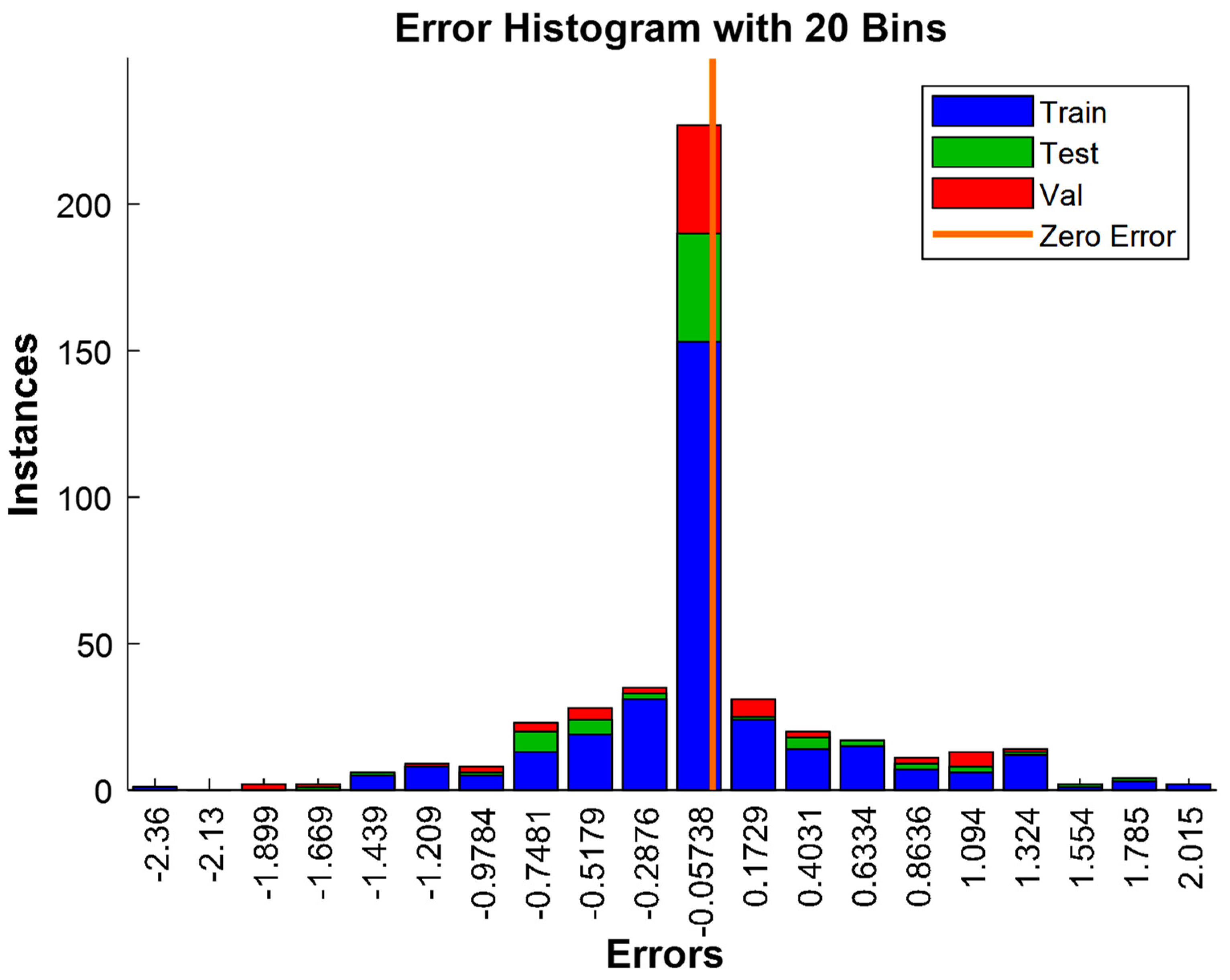
The residual method was applied to strengthen the validation of the optimized DT_DA model. Three complementary approaches were used to assess its accuracy and stability. First, the experimental values were visually compared with the predicted values by superimposing their curves for the entire database, covering the training, validation and testing phases. This representation, presented in Figure 5, allows for a visual assessment of the overall agreement between the model predictions and the observed data. A close superposition of the two curves indicates very good predictive power. The second analysis method consists of plotting the histogram of the distribution of residual errors (deviations between experimental and predicted values), as shown in Figure 6. This approach allows for verifying whether the errors are centered around zero and distributed symmetrically. A normal and centered distribution is a key indicator of reliability and absence of systematic bias in the model predictions. Finally, the third method deepens this analysis by representing the residuals as separate histograms for each phase of the modeling process, namely training, and validation (Figure 7). This visualization allows comparing the dispersion of errors between the different stages and assessing the stability of the model on independent datasets. The integration of these three approaches provides a comprehensive view of the performance of the DT_DA model, both in terms of accuracy and robustness. The results obtained through residual analysis confirm the model’s ability to faithfully reproduce the behavior of real data while maintaining good generalization [47].

Figure 5, Figure 6 and Figure 7 provide a clear and complementary visualization of the performance and robustness of the optimized DT_DA model. Figure 5 displays the superposition of experimental and predicted TAC values for the entire dataset, covering the training, and validation phases. The near-perfect overlap of the two curves demonstrates the excellent predictive capacity of the model, with only negligible deviations across all phases of learning. Figure 6 illustrates the overall distribution of residual errors as a frequency histogram. The highest frequencies are sharply concentrated around zero, while nearly all remaining frequencies fall within the narrow interval of approximately [−2.5, +2.5]. Summing the frequencies within this range yields a total very close to the number of analyzed samples, indicating that the vast majority of predictions exhibit extremely small errors. This tight clustering of residuals near zero provides strong evidence of the model’s high accuracy and reliability. Figure 7 further refines this analysis by showing the error distributions for each data subset (training, and validation) separately. In all three cases, the residuals remain strongly centered around zero with similar spread, confirming that the DT_DA model maintains consistent predictive behavior across all phases. This stability demonstrates the model’s ability to generalize effectively to unseen data, with no indication of overfitting despite the complexity of the decision tree. Together, these figures confirm that the DT_DA model not only achieves excellent predictive performance but also delivers robust and stable predictions across diverse sampling conditions [48].

3.4. Decision Tree

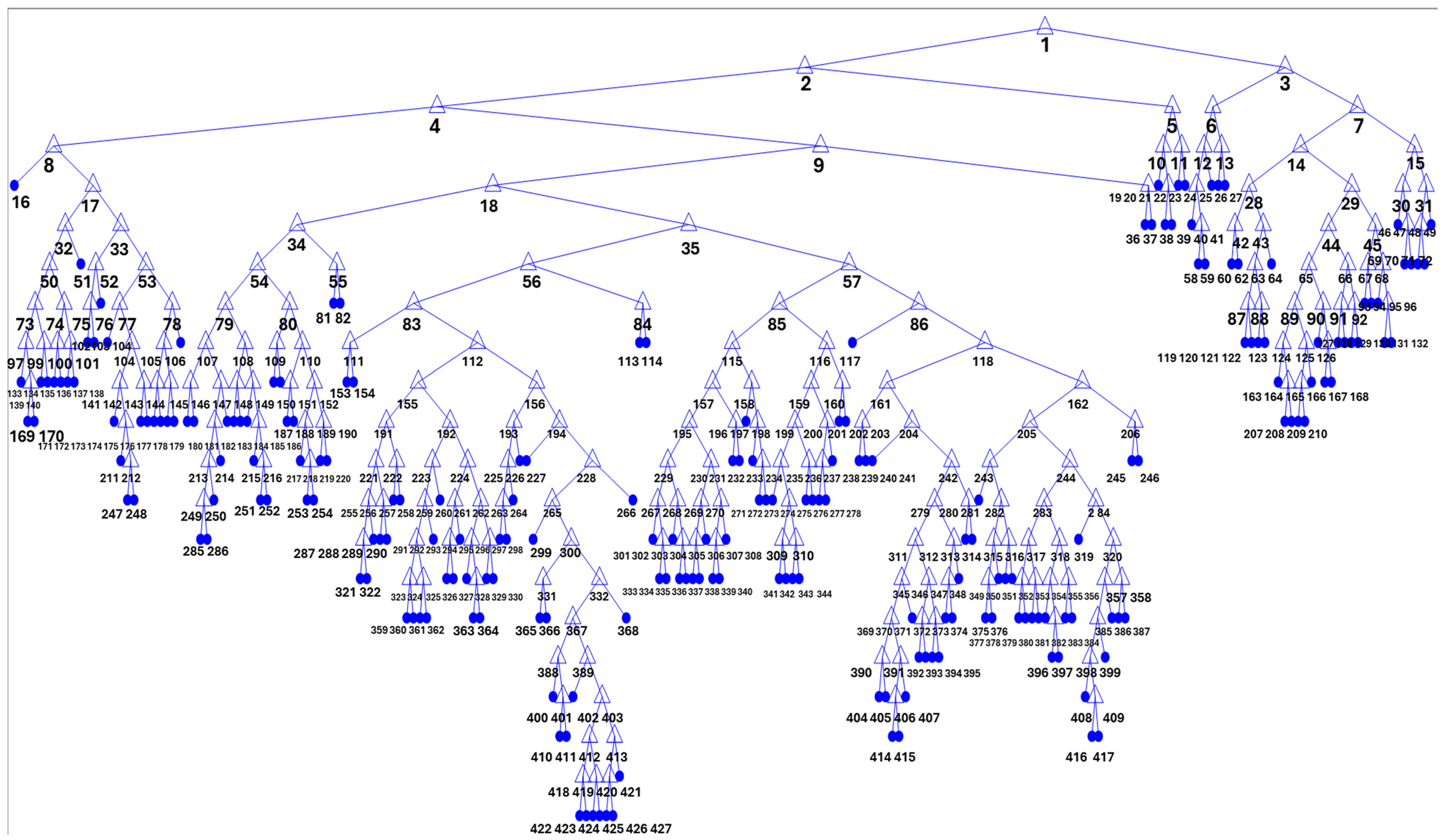
One of the main advantages of this model lies in its ability to explicitly identify the determining parameters, as well as their critical thresholds, having a significant influence, positive or negative [49], on TAC. Thanks to the hierarchical structure of the decision tree, it becomes possible to considerably reduce the need for exhaustive physicochemical analyses. Indeed, the model allows the TAC value to be precisely estimated by examining the most influential variables one by one, following a path conditioned by the prior analytical results. This targeted approach optimizes analytical resources, while providing precise information on the threshold concentrations from which the effects become significant. Details of the decision tree applied to the regression are presented in the Supplementary Data (Table S1).

To evaluate the global influence of each input parameter on TAC, a global feature-importance analysis was carried out using the impurity-based metric intrinsic to the DT. This analysis revealed that total hardness, bicarbonate concentration, and sulfate content were the most influential variables driving TAC prediction, followed by calcium and magnesium concentrations. These results are consistent with the well-known role of carbonate equilibria and hardness in governing pH buffering capacity, thereby reinforcing the chemical interpretability of the model. The feature-importance ranking complements the node-by-node decision rules provided in Figure 8 and the detailed node characteristics listed in Table S1, offering both a global sensitivity perspective and transparent decision criteria.

The decision tree (Figure 8) shows that the most important variable for predicting TAC is water hardness (X4, TH), with a critical threshold at 78.5 °F. This observation is consistent with water chemistry, as hardness, measured primarily by calcium and magnesium concentrations, is strongly correlated with alkaline buffering capacity [50]. When hardness is below 78.5 °F, the tree enters a series of fine-grained decisions based on the concentrations of other major ions, including bicarbonate (X7), chloride (X8), sulfate (X13), and other physicochemical parameters. This reflects the central role of bicarbonates and carbonates in defining TAC, as they are the main contributors to alkalinity [51].

The second important variable involved in the split is bicarbonate concentration (X7), with thresholds around 421.68 mg/L. This threshold appears to distinguish waters with high alkalinity due to high bicarbonate concentrations. This high presence of bicarbonates favors high alkalinity (high TAC), which is expected, since bicarbonates are the compounds responsible for neutralizing acids in water. The concomitant presence of chlorides (X8) is also significant, indicating that waters with a particular ionic balance between bicarbonates and chlorides display different alkalimetric properties [52].

The tree also demonstrates the importance of sulfate (X13) in the modeling. Sulfates, often present in natural water, can modulate the overall ionic composition and indirectly influence hardness and alkalinity [53]. Their role appears in sub-branches where hardness is low but sulfates exceed certain thresholds, which impacts the TAC prediction. Variables such as pH (X3), although less frequently at the top of decisions, also appear, which makes sense given that pH affects the chemical balance between the different forms of carbonate/bicarbonate ions and therefore buffering capacity [54]. Similarly, variables such as electrical conductivity (X1) and dry residue (X19) are involved at depth, reflecting their overall role in the total dissolved ion concentration, characterizing the mineral quality of the water [55,56].

The tree also distinguishes waters with a hardness greater than 78.5 °F, where other ions such as sodium (X14), potassium (X15), manganese (X16), and iron (X17) influence the prediction. These ions can be associated with natural or anthropogenic sources and contribute to the overall ionic composition, significantly modifying the TAC [57].

The prediction values (fit) associated with each leaf of the tree are consistent with what is expected in aquatic systems. Low predictions (e.g., around 10–20 °F) correspond to soft water with low hardness and low alkalinity [58], while high predictions (up to 600 °F and above) correspond to hard water, rich in bicarbonates and other major ions [59]. This wide range reflects the natural diversity of waters and demonstrates that the tree captures this variability well.

Finally, the presence of variables such as organic matter (X20), phosphate (X12), nitrates (X11), ammonium (X10), and nitrites (X9), although less frequent in the first decisions, highlights that these parameters can also indirectly influence overall chemistry and therefore alkalinity, particularly in waters impacted by agricultural or urban activities [60].

All of these observations give the decision tree the ability to accurately and realistically interpret the physicochemical mechanisms governing total alkali content. The model perfectly reflects the complexity of natural water, where the interdependence between different ions and parameters determines the quality and chemical behavior of the environment [61]. Robust prediction of the TAC through this model can thus be used to better understand the dynamics of the waters studied, anticipate their reactions to various treatments and assess their environmental impact, which is crucial for the sustainable management of water resources.

4. Discussion

TAC modeling using a decision tree optimized by the Dragonfly algorithm provides a detailed understanding of the mechanisms that control the chemical stability of aquatic ecosystems [62]. The model’s extraordinary predictive quality, illustrated by correlation and determination coefficients greater than 0.9999 and very low errors, confirms that complex interactions between physicochemical parameters can be described with near-experimental accuracy. This performance demonstrates that an algorithm considered relatively simple, such as a decision tree, can compete with more sophisticated methods while maintaining transparency that allows for direct interpretation of the results [63]. This ability to combine accuracy and readability is a decisive asset for water quality management, particularly in contexts where “black box” models complicate decision-making [64].

Analysis of the importance of variables highlights the predominant role of total hardness and bicarbonate concentration, followed by sulfates and chlorides, in determining TAC. Hardness, a reflection of calcium and magnesium concentrations, acts as a global indicator of water’s buffering capacity [65]. The critical threshold of 78.5 °F highlights a transition between soft water, which is less resistant to pH variations, and harder water, which offers greater resilience to acidic inputs. Similarly, bicarbonate concentration, with a threshold of 421.68 mg L⁻¹, delineates a zone where proton neutralization becomes particularly effective. These thresholds constitute operational references, directly usable for diagnosing the chemical state of a body of water or for guiding management measures. They also reflect the importance of carbonate balances in maintaining pH, in relation to the solubility of calcium and magnesium carbonates and the dynamics of atmospheric CO₂ exchanges [66].

The richness of the database, comprising 454 samples collected over a full year and covering a wide range of environments (springs, rivers, dams, treated water), made it possible to capture rarely documented spatio-temporal variability. This diversity highlighted more subtle interactions than just hardness–bicarbonate relationships. For example, the combined effect of sulfates and hardness, identified in certain branches of the tree, shows that anions such as SO₄²⁻, although not directly contributing to alkalinity, can modify the overall ionic balance and indirectly influence buffering capacity. The recurring presence of chlorides and, to a lesser extent, sodium or potassium in the terminal decisions underscores the impact of total ionicity, as expressed by electrical conductivity, on the distribution of carbonate species. Such relationships, often nonlinear, would be difficult to reveal using conventional statistical approaches [67].

The model not only reproduces known relationships; it also offers diagnostic tools to optimize monitoring strategies. Thanks to its hierarchical structure, it is possible to predict alkalinity based on a limited number of parameters, thus reducing analytical requirements without significant loss of accuracy [68]. This capability represents a considerable economic and practical advantage for water resource managers, particularly in regions where sampling and analysis campaigns are costly or limited by logistical constraints. The decision tree allows, for example, to focus efforts on measuring hardness and bicarbonate, two key variables that determine most critical thresholds [69].

Beyond the purely analytical aspects, the environmental implications of these results are particularly important. Alkalinity prediction provides leverage to anticipate episodes of pH instability, which can be triggered by acidic inputs linked to industrial discharges, acid precipitation, or the decomposition of organic matter [70]. By identifying the most vulnerable systems in advance, the model helps prevent impacts on aquatic biodiversity, particularly by limiting pH fluctuations that could affect nutrient availability, heavy metal solubility, or the enzymatic activity of microorganisms. The identified thresholds can serve as benchmarks for water quality monitoring, treatment plan design, or risk assessment in climate change contexts where extreme events (droughts, intense rainfall) alter ion balances.

The model’s ability to link routine physicochemical variables to an integrating property such as alkalinity also opens up prospects for transfer to other regions or types of environments. Although developed using data collected in the Médéa region, this methodological framework could be applied to watersheds with comparable geochemical conditions, subject to a recalibration phase. The future integration of broader environmental factors, such as land use, agricultural intensity, or proximity to industrial sources, would make it possible to directly link chemical determinants to anthropogenic pressures. Such an extension would strengthen the model’s predictive capacity and make it a decision-support tool for environmental planning, water resource protection, and adaptation to the impacts of climate change [71].

In summary, this study demonstrates that a transparent and high-performance modeling approach can provide both reliable predictions and a mechanistic understanding of the processes that govern the acid–base balance of natural waters. By highlighting critical thresholds and complex interactions between major ions, the model constitutes a robust tool for anticipating risks of chemical imbalance and guiding sustainable management strategies for aquatic ecosystems.

5. Conclusions

This study successfully developed and validated a robust and interpretable decision tree model for predicting total alkalinity (TAC) in aquatic systems. Trained on a dataset of 454 samples and incorporating twenty physicochemical parameters, the optimized model achieved outstanding predictive performance with a correlation coefficient R of 0.9999 and minimal prediction errors (RMSE = 0.3957, MAE = 0.3572, and MAPE = 0.4531). External validation using 68 independent data points further confirmed the model’s generalization ability (R = 0.9999; RMSE = 0.4223; MAE = 0.3871, and MAPE = 0.4931), demonstrating its reliability in real-world applications. The model not only provides accurate predictions but also identifies of the most influential variables affecting TAC. Specifically, total hardness (X4 ≥ 78.5 °F), bicarbonate concentrations (X7 ≥ 421.68 mg/L), and sulfates and chlorides emerged as key contributors. The hierarchical structure of the decision tree highlights critical thresholds and interactions between variables, offering insights into the buffering mechanisms of water bodies. The integration of the Dragonfly optimization algorithm enabled fine-tuning of the model’s complexity, avoiding overfitting while maximizing performance. Furthermore, residual analyses confirmed the normality, stability, and reliability of the model across all phases—training, validation, and testing. This predictive model thus represents a powerful decision-support tool for water managers, enabling the anticipation of pH instability, the optimization of analytical resources, and the formulation of targeted interventions for ecosystem protection. Its interpretability makes it particularly suitable for operational use in environmental monitoring and sustainable water resource management. As a perspective, future work will focus on integrating broader environmental and anthropogenic drivers such as point- and non-point source pollution, agricultural practices, industrial activities, and human disturbances into the modeling framework. This extension will strengthen the connection between the direct physicochemical determinants of TAC and their underlying causes, thereby enhancing the usefulness of the model for management-oriented applications and policy-making.

References

1. Kasper, S.; Adeyemo, O.K.; Becker, T.; Scarfe, D.; Tepper, J. Aquatic Environment and Life Support Systems. In Fundamentals of Aquatic Veterinary Medicine; John Wiley & Sons Ltd.: Hoboken, NJ, USA, 2022. [Google Scholar]
2. Pandey, P.K.; Pande, A. Aquatic Environment Management; CRC Press: Boca Raton, FL, USA, 2023. [Google Scholar]
3. De Paiva Magalhães, D.; Da Costa Marques, M.R.; Baptista, D.F.; Buss, D.F. Metal Bioavailability and Toxicity in Freshwaters. Environ. Chem. Lett. 2015, 13, 69–87. [Google Scholar] [CrossRef]
4. Elder, J.F. Metal Biogeochemistry in Surface-Water Systems: A Review of Principles and Concepts; Geological Survey (U.S.): Reston, VA, USA, 1988. [Google Scholar]
5. Babaniyi, G.G.; Olagoke, O.V.; Aransiola, S.A. Extracellular Enzymatic Activity of Bacteria in Aquatic Ecosystems. In Microbiology for Cleaner Production and Environmental Sustainability; CRC Press: Boca Raton, FL, USA, 2023; pp. 277–300. [Google Scholar]
6. Chu, Y.; Zhang, X.; Tang, X.; Jiang, L.; He, R. Uncovering Anaerobic Oxidation of Methane and Active Microorganisms in Landfills by Using Stable Isotope Probing. Environ. Res. 2025, 271, 121139. [Google Scholar] [CrossRef]
7. Muniz, I.P. Freshwater Acidification: Its Effects on Species and Communities of Freshwater Microbes, Plants and Animals. Proc. R. Soc. Edinb. Sect. B Biol. Sci. 1990, 97, 227–254. [Google Scholar] [CrossRef]
8. Tahraoui, H.; Toumi, S.; Boudoukhani, M.; Touzout, N.; Sid, A.N.E.H.; Amrane, A.; Belhadj, A.-E.; Hadjadj, M.; Laichi, Y.; Aboumustapha, M. Evaluating the Effectiveness of Coagulation–Flocculation Treatment Using Aluminum Sulfate on a Polluted Surface Water Source: A Year-Long Study. Water 2024, 16, 400. [Google Scholar] [CrossRef]
9. Fraga, C.G.; Oteiza, P.I.; Galleano, M. In Vitro Measurements and Interpretation of Total Antioxidant Capacity. Biochim. Biophys. Acta (BBA)-Gen. Subj. 2014, 1840, 931–934. [Google Scholar] [CrossRef]
10. Tahraoui, H.; Belhadj, A.-E.; Moula, N.; Bouranene, S.; Amrane, A. Optimisation and Prediction of the Coagulant Dose for the Elimination of Organic Micropollutants Based on Turbidity. Kemija u industriji 2021, 70, 675–691. [Google Scholar] [CrossRef]
11. Jothivenkatachalam, K.; Nithya, A.; Mohan, S.C. Correlation Analysis of Drinking Water Quality in and around Perur Block of Coimbatore District, Tamil Nadu, India. Rasayan J. Chem. 2010, 3, 649–654. [Google Scholar]
12. Regadío, M.; De Soto, I.S.; Rodríguez-Rastrero, M.; Ruiz, A.I.; Gismera, M.J.; Cuevas, J. Processes and Impacts of Acid Discharges on a Natural Substratum under a Landfill. Sci. Total Environ. 2013, 463, 1049–1059. [Google Scholar] [CrossRef]
13. Tuck, I.D.; Pinkerton, M.H.; Tracey, D.M.; Anderson, O.F.; Chiswell, S.M. Ecosystem and Environmental Indicators for Deepwater Fisheries; Ministry for Primary Industries: Wellington, New Zealand, 2014.
14. Tahraoui, H.; Belhadj, A.E.; Hamitouche, A.E. Prediction of the Bicarbonate Amount in Drinking Water in the Region of Médéa Using Artificial Neural Network Modelling. Kemija u industriji 2020, 69, 595–602. [Google Scholar] [CrossRef]
15. Floegel, A.; Kim, D.-O.; Chung, S.-J.; Song, W.O.; Fernandez, M.L.; Bruno, R.S.; Koo, S.I.; Chun, O.K. Development and Validation of an Algorithm to Establish a Total Antioxidant Capacity Database of the US Diet. Int. J. Food Sci. Nutr. 2010, 61, 600–623. [Google Scholar] [CrossRef]
16. Wei, C.; Zhao, T.; Cao, J.; Li, P. Water Quality Prediction Model Based on Interval Type-2 Fuzzy Neural Network with Adaptive Membership Function. Int. J. Fuzzy Syst. 2025. [Google Scholar] [CrossRef]
17. Mehrotra, D. Basics of Artificial Intelligence & Machine Learning; Notion Press: Chennai, India, 2019. [Google Scholar]
18. Surden, H. Machine Learning and Law: An Overview. In Research Handbook on Big Data Law; Edward Elgar Publishing: Cheltenham, UK, 2021; pp. 171–184. [Google Scholar]
19. Wang, Z.; Wang, Q.; Yang, F.; Wang, C.; Yang, M.; Yu, J. How Machine Learning Boosts the Understanding of Organic Pollutant Adsorption on Carbonaceous Materials: A Comprehensive Review with Statistical Insights. Sep. Purif. Technol. 2024, 350, 127790. [Google Scholar] [CrossRef]
20. Tahraoui, H.; Toumi, S.; Hassein-Bey, A.H.; Bousselma, A.; Sid, A.N.E.H.; Belhadj, A.-E.; Triki, Z.; Kebir, M.; Amrane, A.; Zhang, J. Advancing Water Quality Research: K-Nearest Neighbor Coupled with the Improved Grey Wolf Optimizer Algorithm Model Unveils New Possibilities for Dry Residue Prediction. Water 2023, 15, 2631. [Google Scholar] [CrossRef]
21. James, G.; Witten, D.; Hastie, T.; Tibshirani, R.; Taylor, J. Tree-Based Methods. In An Introduction to Statistical Learning; Springer Texts in Statistics; Springer International Publishing: Cham, Switzerland, 2023; pp. 331–366. ISBN 978-3-031-38746-3. [Google Scholar]
22. Rodier, J.; Geoffray, C.; Rodi, L. L’analyse de l’eau: Eaux Naturelles, Eaux Residuaires, Eau de Mer: Chimie, Physico-Chimie, Bacteriologie, Biologie; Dunod: Paris, France, 1996. [Google Scholar]
23. Zhao, Y.; Wang, H.; Song, B.; Xue, P.; Zhang, W.; Peth, S.; Hill, R.L.; Horn, R. Characterizing Uncertainty in Process-Based Hydraulic Modeling, Exemplified in a Semiarid Inner Mongolia Steppe. Geoderma 2023, 440, 116713. [Google Scholar] [CrossRef]
24. Costa, V.G.; Pedreira, C.E. Recent Advances in Decision Trees: An Updated Survey. Artif. Intell. Rev. 2023, 56, 4765–4800. [Google Scholar] [CrossRef]
25. Priyanka, N.A.; Kumar, D. Decision Tree Classifier: A Detailed Survey. Int. J. Inf. Decis. Sci. 2020, 12, 246. [Google Scholar] [CrossRef]
26. Gupta, B.; Rawat, A.; Jain, A.; Arora, A.; Dhami, N. Analysis of Various Decision Tree Algorithms for Classification in Data Mining. Int. J. Comput. Appl. 2017, 163, 15–19. [Google Scholar] [CrossRef]
27. Miller, D.W. Results of a New Classification Algorithm Combining K Nearest Neighbors and Recursive Partitioning. J. Chem. Inf. Comput. Sci. 2001, 41, 168–175. [Google Scholar] [CrossRef]
28. Hsieh, W.W. Machine Learning Methods in the Environmental Sciences: Neural Networks and Kernels; Cambridge University Press: Cambridge, UK, 2009. [Google Scholar]
29. Workie, M.D.; Hailu, B.T.; Birhanu, B.; Suryabhagavan, K.V. Statistical Analysis of Earth Observing Data for Physicochemical Water Quality Parameters Estimation for Lake Beseka, Northern Main Ethiopian Rift, Ethiopia. Geol. Ecol. Landsc. 2024, 1–21. [Google Scholar] [CrossRef]
30. Chelghoum, H.; Nasrallah, N.; Tahraoui, H.; Seleiman, M.F.; Bouhenna, M.M.; Belmeskine, H.; Zamouche, M.; Djema, S.; Zhang, J.; Mendil, A. Eco-Friendly Synthesis of ZnO Nanoparticles for Quinoline Dye Photodegradation and Antibacterial Applications Using Advanced Machine Learning Models. Catalysts 2024, 14, 831. [Google Scholar] [CrossRef]
31. Guediri, A.; Bouguettoucha, A.; Tahraoui, H.; Chebli, D.; Zhang, J.; Amrane, A.; Khezami, L.; Assadi, A.A. The Enhanced Adsorption Capacity of Ziziphus Jujuba Stones Modified with Ortho-Phosphoric Acid for Organic Dye Removal: A Gaussian Process Regression Approach. Water 2024, 16, 1208. [Google Scholar] [CrossRef]
32. Auret, L.; Aldrich, C. Interpretation of Nonlinear Relationships between Process Variables by Use of Random Forests. Miner. Eng. 2012, 35, 27–42. [Google Scholar] [CrossRef]
33. Kyriazos, T.; Poga, M. Application of Machine Learning Models in Social Sciences: Managing Nonlinear Relationships. Encyclopedia 2024, 4, 1790–1805. [Google Scholar] [CrossRef]
34. Yang, Y.; Morillo, I.G.; Hospedales, T.M. Deep Neural Decision Trees. arXiv 2018, arXiv:1806.06988. [Google Scholar] [CrossRef]
35. Shang, Y.; Song, K.; Wen, Z.; Lai, F.; Liu, G.; Tao, H.; Yu, X. Machine Learning Reveals Distinct Aquatic Organic Matter Patterns Driven by Soil Erosion Types. Environ. Sci. Ecotechnol. 2025, 25, 100570. [Google Scholar] [CrossRef]
36. Hussain, J. Deep Learning Black Box Problem. 2019. Available online: https://www.diva-portal.org/smash/record.jsf?pid=diva2%3A1353609&dswid=9433 (accessed on 25 June 2025).
37. Abellán, J.; Masegosa, A.R. Bagging Decision Trees on Data Sets with Classification Noise. In Foundations of Information and Knowledge Systems; Link, S., Prade, H., Eds.; Lecture Notes in Computer Science; Springer: Berlin/Heidelberg, Germany, 2010; Volume 5956, pp. 248–265. ISBN 978-3-642-11828-9. [Google Scholar]
38. Fritz, M. Decision Tree Classification with Missing Values. Ph.D. Thesis, Technische Universität Wien, Vienna, Austria, 2023. [Google Scholar]
39. García, S.; Luengo, J.; Herrera, F. Data Preprocessing in Data Mining; Intelligent Systems Reference Library; Springer International Publishing: Cham, Switzerland, 2015; Volume 72, ISBN 978-3-319-10246-7. [Google Scholar]
40. Boorman, D.B.; Hollis, J.M.; Lilly, A. Hydrology of Soil Types: A Hydrologically-Based Classification of the Soils of United Kingdom; Institute of Hydrology: Roorkee, India, 1995. [Google Scholar]
41. Pan, W.; Chen, J.; Lv, B.; Peng, L. Lightweight Marine Biodetection Model Based on Improved YOLOv10. Alex. Eng. J. 2025, 119, 379–390. [Google Scholar] [CrossRef]
42. Abdelmonaim, M.; Radouane, E.M.; Abdelkader, C.; Mourad, D.; Youssef, O.; Abderrazzaq, B.; Mhamed, K.; Taouraout, A. Evaluating the Quality of Groundwater in the Zagora Region, Southeast Morocco, Using GIS and the Water Quality Index (WQI). Geol. Ecol. Landsc. 2024, 1–17. [Google Scholar] [CrossRef]
43. Tahraoui, H.; Belhadj, A.-E. Optimisation de l’élimination Des Micropolluants Organiques. Ph.D. Thesis, Université de Lille, Lille, France, 2021. [Google Scholar]
44. Tahraoui, H.; Belhadj, A.-E.; Hamitouche, A.; Bouhedda, M.; Amrane, A. Predicting the Concentration of Sulfate (SO42−) in Drinking Water Using Artificial Neural Networks: A Case Study: Médéa-Algeria. Desalination Water Treat. 2021, 217, 181–194. [Google Scholar] [CrossRef]
45. Nedjhioui, M.; Nasrallah, N.; Kebir, M.; Tahraoui, H.; Bouallouche, R.; Assadi, A.A.; Amrane, A.; Jaouadi, B.; Zhang, J.; Mouni, L. Designing an efficient surfactant–polymer–oil–electrolyte system: A multi-objective optimization study. Processes 2023, 11, 1314. [Google Scholar] [CrossRef]
46. Li, F.; Lu, H.; Wang, G.; Qiu, J. Long-Term Capturability of Atmospheric Water on a Global Scale. Water Resour. Res. 2024, 60, e2023WR034757. [Google Scholar] [CrossRef]
47. Pang, Q.; Zhao, G.; Wang, D.; Zhu, X.; Xie, L.; Zuo, D.; Wang, L.; Tian, L.; Peng, F.; Xu, B. Water Periods Impact the Structure and Metabolic Potential of the Nitrogen-Cycling Microbial Communities in Rivers of Arid and Semi-Arid Regions. Water Res. 2024, 267, 122472. [Google Scholar] [CrossRef] [PubMed]
48. Wang, P.; Li, J.; An, P.; Yan, Z.; Xu, Y.; Pu, S. Enhanced Delivery of Remedial Reagents in Low-Permeability Aquifers through Coupling with Groundwater Circulation Well. J. Hydrol. 2023, 618, 129260. [Google Scholar] [CrossRef]
49. Tong, H. Threshold Models in Non-Linear Time Series Analysis; Springer Science & Business Media: Heidelberg, Germany, 2012; Volume 21. [Google Scholar]
50. Islam, M.S.; Majumder, S. Alkalinity and Hardness of Natural Waters in Chittagong City of Bangladesh. Int. J. Sci. Bus. 2020, 4, 137–150. [Google Scholar]
51. Müller, B.; Meyer, J.S.; Gächter, R. Alkalinity Regulation in Calcium Carbonate-Buffered Lakes: Alkalinity Regulation in Calcium Carbonate-Buffered Lakes. Limnol. Oceanogr. 2016, 61, 341–352. [Google Scholar] [CrossRef]
52. Casado, Á.; Ramos, P.; Rodríguez, J.; Moreno, N.; Gil, P. Types and Characteristics of Drinking Water for Hydration in the Elderly. Crit. Rev. Food Sci. Nutr. 2015, 55, 1633–1641. [Google Scholar] [CrossRef]
53. Menon, S.V.; Kumar, A.; Middha, S.K.; Paital, B.; Mathur, S.; Johnson, R.; Kademan, A.; Usha, T.; Hemavathi, K.N.; Dayal, S. Water Physicochemical Factors and Oxidative Stress Physiology in Fish, a Review. Front. Environ. Sci. 2023, 11, 1240813. [Google Scholar] [CrossRef]
54. Legarra, M.; Blitz, A.; Czégény, Z.; Antal, M.J. Aqueous Potassium Bicarbonate/Carbonate Ionic Equilibria at Elevated Pressures and Temperatures. Ind. Eng. Chem. Res. 2013, 52, 13241–13251. [Google Scholar] [CrossRef]
55. Corwin, D.L.; Yemoto, K. Salinity: Electrical Conductivity and Total Dissolved Solids. Soil Sci. Soc. Am. J. 2020, 84, 1442–1461. [Google Scholar] [CrossRef]
56. Atanacković, N.; Dragišić, V.; Stojković, J.; Papić, P.; Živanović, V. Hydrochemical Characteristics of Mine Waters from Abandoned Mining Sites in Serbia and Their Impact on Surface Water Quality. Environ. Sci. Pollut. Res. 2013, 20, 7615–7626. [Google Scholar] [CrossRef]
57. Laaraj, M.; Benaabidate, L.; Mesnage, V.; Lahmidi, I. Assessment and Modeling of Surface Water Quality for Drinking and Irrigation Purposes Using Water Quality Indices and GIS Techniques in the Inaouene Watershed, Morocco. Model. Earth Syst. Environ. 2024, 10, 2349–2374. [Google Scholar] [CrossRef]
58. Bogart, S.J.; Woodman, S.; Steinkey, D.; Meays, C.; Pyle, G.G. Rapid Changes in Water Hardness and Alkalinity: Calcite Formation Is Lethal to Daphnia Magna. Sci. Total Environ. 2016, 559, 182–191. [Google Scholar] [CrossRef]
59. Sengupta, P. Potential Health Impacts of Hard Water. Int. J. Prev. Med. 2013, 4, 866. [Google Scholar]
60. Abbasi, T.; Abbasi, S.A. Water Quality Indices; Elsevier: Amsterdam, The Netherlands, 2012. [Google Scholar]
61. Guo, T.; Yue, Q.; Hou, Y.; Chen, Y.; Yu, D.; Yang, G.; Yu, C.; Zeng, Y.; Feng, Y.; Pu, S. Unveiling the Overlooked Silent Threat: High-Throughput Suspect Screening of Antibiotics and Multidimensional Heterogeneity in Aquatic Ecosystems of Megacity. J. Hazard. Mater. 2025, 493, 138193. [Google Scholar] [CrossRef]
62. Randive, P.; Bhagat, M.S.; Bhorkar, M.P.; Bhagat, R.M.; Vinchurkar, S.M.; Shelare, S.; Sharma, S.; Beemkumar, N.; Hemalatha, S.; Kumar, P. Adaptive Optimization of Natural Coagulants Using Hybrid Machine Learning Approach for Sustainable Water Treatment. Sci. Rep. 2025, 15, 16096. [Google Scholar] [CrossRef]
63. Blockeel, H.; Devos, L.; Frénay, B.; Nanfack, G.; Nijssen, S. Decision Trees: From Efficient Prediction to Responsible AI. Front. Artif. Intell. 2023, 6, 1124553. [Google Scholar] [CrossRef] [PubMed]
64. Haasnoot, M. Anticipating Change: Sustainable Water Policy Pathways for an Uncertain Future. Ph.D. Thesis, University of Twente, Enschede, The Netherlands, 2013. [Google Scholar]
65. Zegaar, A. Classification of Irrigation Water Based on Machine Learning Approach. Ph.D. Thesis, University of Biskra, Biskra, Algeria, 2025. [Google Scholar]
66. Santos, H.S.; Nguyen, H.; Venâncio, F.; Ramteke, D.; Zevenhoven, R.; Kinnunen, P. Mechanisms of Mg Carbonates Precipitation and Implications for CO2 Capture and Utilization/Storage. Inorg. Chem. Front. 2023, 10, 2507–2546. [Google Scholar] [CrossRef]
67. Thakur, A.; Kumar, A. Electrochemistry Basics and Theory of Scaling in Various Electrolytes: Effect of pH and Other Parameters. In Industrial Scale Inhibition; Yaagoob, I.Y., Verma, C., Eds.; Wiley: Hoboken, NJ, USA, 2024; pp. 36–71. ISBN 978-1-394-19117-8. [Google Scholar]
68. Pang, H.; Ben, Y.; Cao, Y.; Qu, S.; Hu, C. Time Series-Based Machine Learning for Forecasting Multivariate Water Quality in Full-Scale Drinking Water Treatment with Various Reagent Dosages. Water Res. 2025, 268, 122777. [Google Scholar] [CrossRef]
69. Sheffield, J.; Wood, E.F.; Pan, M.; Beck, H.; Coccia, G.; Serrat-Capdevila, A.; Verbist, K. Satellite Remote Sensing for Water Resources Management: Potential for Supporting Sustainable Development in Data-Poor Regions. Water Resour. Res. 2018, 54, 9724–9758. [Google Scholar] [CrossRef]
70. Krivtsov, V. Investigations of Indirect Relationships in Ecology and Environmental Sciences: A Review and the Implications for Comparative Theoretical Ecosystem Analysis. Ecol. Model. 2004, 174, 37–54. [Google Scholar] [CrossRef]
71. Harmel, R.D.; Chaubey, I.; Ale, S.; Nejadhashemi, A.P.; Irmak, S.; DeJonge, K.C.; Evett, S.R.; Barnes, E.M.; Catley-Carlson, M.; Hunt, S. Perspectives on Global Water Security. Trans. ASABE 2020, 63, 69–80. [Google Scholar] [CrossRef]
Figure 1. Mapping of sampling points.
Water 17 02939 g001
Figure 2. Organization chart for the development and optimization of the decision tree model.
Water 17 02939 g002
Figure 3. Comparison between experimental and predicted values of DT_DA model: (a) training phase, (b) validation phase, and (c) All phase.
Water 17 02939 g003aWater 17 02939 g003b
Figure 4. Relationship between experimental and predicted values to assess performance.
Water 17 02939 g004
Figure 5. Overlay of experimental and predicted values from the DT_DA model for the entire dataset (training and validation).
Water 17 02939 g005
Figure 6. Distribution of residual errors from the DT_DA model as a histogram for the entire dataset.
Water 17 02939 g006
Figure 7. Separate histograms of residual errors for the training, validation, and testing phases of the DT_DA model.
Water 17 02939 g007
Figure 8. The decision tree for TAC.
Water 17 02939 g008